Abstract
Humanitarian logistics in response to large scale disasters entails decisions that must be taken urgently and under high uncertainty. In addition, the scarcity of available resources sometimes causes the involved organizations to suffer assaults while transporting the humanitarian aid. This paper addresses the last mile distribution problem that arises in such an insecure environment, in which vehicles are often forced to travel together forming convoys for security reasons. We develop an elaborated methodology based on Ant Colony Optimization that is applied to two case studies built from real disasters, namely the 2010 Haiti earthquake and the 2005 Niger famine. There are very few works in the literature dealing with problems in this context, and that is the research gap this paper tries to fill. Furthermore, the consideration of multiple criteria such as cost, time, equity, reliability, security or priority, is also an important contribution to the literature, in addition to the use of specialized ants and effective pheromones that are novel elements of the algorithm which could be exported to other similar problems. Computational results illustrate the efficiency of the new methodology, confirming it could be a good basis for a decision support tool for real operations.
1. Introduction
Disaster management remains a crucial challenge for the international community. National and supranational institutions and non-governmental organizations have to deal with high impact disasters such as the 2010 Haiti earthquake, the 2013 Typhoon Haiyan or the 2018 Sulawesi earthquake and tsunami. This global concern is reflected in the scientific literature and specifically in the Operations Research community, where the increasing interest on humanitarian logistics and disaster management entails the publication of surveys [1,2], books [3,4], special issues [5,6] and journals (such as the Journal of Humanitarian Logistics and Supply Chain Management).
Within the disaster management cycle, the response phase includes the actions to be performed once the disaster has occurred. Research on the response phase may focus on specific types of disasters, such as earthquakes [7,8] or floods [9], or can address particular problems for generic disasters, such as location-allocation [10], evacuation [11], or debris management [12]. Among the operations to be carried out after a disaster strikes, the distribution of aid to the affected people plays an important role. Along with the usual objectives in commercial logistics, mainly the operation cost, in humanitarian logistics other attributes have to be considered [13,14], such as the response time, the equity of the distribution, etc. Therefore, multi-criteria models are necessary to face many realistic problems in this context. Gutjahr and Nolz [15] provide a review on multi-criteria decision making in humanitarian aid classifying the existing models as deterministic or stochastic and pre-disaster or post-disaster.
Many times the distribution operations must be performed under unsecure conditions [6]. Assaults to relief vehicles are sadly frequent and this complicates the work of organizations that execute the aid missions. Avoiding as much as possible the most dangerous roads and forcing the vehicles to travel together forming convoys are two ways of improving the security of the operations.
In this paper, we develop an algorithm based on Ant Colony Optimization (ACO) metaheuristic to solve the multi-criteria last mile distribution problem in an unsecure environment stated in [16]. The complexity of this problem makes it necessary to use a heuristic approach to solve realistic cases. Besides, due to the strong links between the elements of a solution, it is difficult to develop heuristics that perform progressive alterations of a solution while ensuring feasibility, as it is the case of evolutionary algorithms or local search heuristics. Instead, algorithms based on construction of solutions, such as Greedy Randomized Adaptive Search Algorithm (GRASP) or Ant Colony Optimization metaheuristics, fit much better.
The ACO methodology that we propose in this work presents some novelties that make it suitable for routing and distribution problems in which the vehicles must travel in convoys. The use of convoys is appropriate not only in humanitarian operations, but in any logistics operation performed in an environment of insecurity, in which attacks on delivery vehicles to steal the commodities are possible. The algorithm considers two types of ants—vehicles and aid kits—four types of standard pheromones, and especially the use of effective pheromones, updatable in the course of each solution building process. This new concept allows a better balance between the elements of a solution and a higher diversification in the set of solutions that can be built. Effective pheromones may be applied to a wide variety of problems, especially vehicle routing problems involving a large number of vehicles. The results obtained show that the new ACO Algorithm proposed in this paper is a useful decision aid tool. The ACO Algorithm provides good quality solutions in a short time in realistic test cases, frequently improving the solutions obtained with the GRASP Algorithm developed in [16].
The rest of this paper is organized as follows. Section 2 reviews the relevant literature on multi-criteria optimization for the last mile distribution problem, as well as some applications of Ant Colony Optimization in disaster management. Section 3 presents the problem of transportation for last mile distribution, including the data notation and the description of the six attributes considered. Section 4 introduces the heuristic method proposed to solve the problem. An Ant Colony Optimization algorithm is developed together with the subordinate procedure that guides the construction of feasible solutions. Section 5 is devoted to showing and analyzing the results obtained when applying the proposed metaheuristic to solve two test cases based on real disasters. Finally, Section 6 draws some conclusions derived from this work.
2. Literature Review
Some of the most significant papers that apply multi-criteria techniques in humanitarian last mile distribution are mentioned below and summarized in Table 1. Viswanath and Peeta [8] develop a multicommodity mixed integer programming model in order to maximize the total population covered and minimize the total travel time for earthquake response. Balcik et al. [17] present a multicommodity, multimodal and multiperiod last mile distribution problem and establish a scalar objective function that aggregates minimization of transportation costs and maximization of demand covered. Nolz et al. [18] consider three attributes (reliability of the transporting tours, coverage and total travel time) in a distribution problem where infrastructure may be damaged in a post-disaster situation. Lin et al. [19] use the scalarization approach to deal with a three-objective (total unsatisfied demand, total travel time and equity of the distribution) integer programming model that allows split deliveries. Two heuristic methods are proposed to solve the model. Bozorgi-Amiri et al. [20] propose a robust stochastic compromise programming model for disaster relief logistics, minimizing the sum of the expected value and the variance of the total cost and minimizing the sum of the maximum unsatisfied demands. Tirado et al. [21] consider four attributes (amount of aid distributed, time of the operation, equity and cost) in a dynamic flow model that is solved via lexicographical goal programming. Huang et al. [22] develop a quadratic multi-objective programming model to face an allocation and distribution problem. Three attributes are considered: lifesaving utility, delay cost and equity of the distribution. This model allows vehicles to visit a node more than once and provides the individual itineraries of the vehicles. Ahmadi et al. [23] aggregate the distribution time, the penalty cost of unsatisfied demand and the costs of opening distribution centers into a single objective function for a location-routing problem considering network failure, random travel times and multiple uses of vehicles. Zhou et al. [24] apply a multi-objective evolutionary algorithm to solve a multiperiod and multicommodity distribution model which aims to minimize the unsatisfied demand and to minimize the risk of choosing damaged roads. Maghfiroh and Hanaoka [25] present a multimodal model considering dynamic and stochastic demands in order to minimize the travel time and the unmet demand. Moreno et al. [26] develop a biobjective multiperiod stochastic location-transportation model that allows multiple trips to the vehicles not only in different periods, but also in the same period. The authors propose different heuristic techniques to solve the model. Outside the scope of aid distribution, Habib et al. [27] address a post-disaster waste management problem through a possibilistic programming model that minimizes both the cost of waste processing and the carbon emissions and maximizes the job opportunities.

Table 1.
The literature related to multi-criteria techniques in humanitarian last mile distribution.
Despite the frequency with which aid distribution is to be carried out in unsafe conditions, only a few papers consider the security as an attribute. Ortuno et al. [28] integrate seven attributes (quantity distributed, time of response, cost, equity, priority, reliability and security) into a linear lexicographical goal programming flow model. This model is multimodal, multidepot, allows split deliveries and vehicles travel in convoys so that they can be escorted. An alternative version of this model is established in Vitoriano et al. [29], where the authors set a fixed amount to distribute and combine the six remaining attributes into a non-lexicographical model. Nevertheless, these models do not provide the individual route of each vehicle, so it is not possible to easily implement plans for the relief distribution. Ferrer et al. [16] propose a GRASP metaheuristic to solve a nonlinear multi-objective model that allows vehicles to visit a node more than once and provides the individual itineraries of the vehicles. The mathematical formulation of this model is established in Ferrer et al. [30], where an extensive comparison of the characteristics of the models is made with other studies that deal with the last mile distribution problem.
In this study, we propose an Ant Colony Optimization methodology to solve the model developed in [16] and [30]. Even though ACO has been applied frequently to different routing and distribution problems [31,32,33,34], it has barely been used in the context of disaster management. The most remarkable work is Yi and Kumar [35], where the authors apply this metaheuristic to solve a distribution and evacuation problem. More recently, Saeidian et al. [36] combine different techniques, including ACO, to face a location-allocation problem of relief centers after an earthquake. Therefore, this paper presents the first application of Ant Colony Optimization to a multi-criteria last mile distribution problem. Furthermore, the proposed ACO methodology introduces novelties such as specialized ants, representing both vehicles and aid kits, and effective pheromones, that conveniently balance the elements of the built solutions.
3. Problem Description
The last mile distribution problem addressed in this paper consists in deciding how to deal out a predetermined amount of humanitarian aid from distribution centers to populations in need by moving a set of vehicles through a transportation network. We consider that the distribution is performed in an insecure and uncertain environment and, as a consequence, the convoys transporting the aid may be attacked while traveling and some roads may be unavailable due to damages produced by the disaster.
Table 2 lists the notation used to represent the main elements of the problem. The transportation network is formed by nodes and arcs. Each node is of one of three types: supply, demand or connection. A supply node represents a distribution center where a certain known amount of aid is available, while the demand nodes represent populations in need or help centers. Each demand node is associated with a certain amount of aid that is desirable to receive and a priority level. A connection node represents an intermediate point, where there is neither available nor demanded aid, but may be used by the vehicles for aid trans-shipment.
Table 2.
Problem notation.
The arcs represent links (roads, pathways, streets, etc.) connecting the nodes. The links that can be traversed in both directions have two associated arcs, one for each direction. Each arc has associated a length, a speed, an assault probability and a probability of being available (the arc can be used).
The vehicles are initially located at some nodes, which are not necessarily supply nodes. We will call depots to the nodes where there are vehicles at the beginning of the operation. There are different types of vehicles to carry out the distribution. Vehicles of the same type have the same capacity, velocity and costs. For technical reasons, we classify the vehicles in classes: vehicles belonging to a same class are of the same type and are located also in the same depot.
The humanitarian aid is packed in kits composed of water, food, medicines, blankets, etc. The operation to be performed consists of delivering of such kits.
In addition, the design of the routes must be carried out under the following assumptions:
- -
- Vehicles can visit a node more than once. Likewise, they can pick up or deliver humanitarian aid more than once, even in the same node.
- -
- Transhipment of aid between vehicles can be made at any node.
- -
- Split pick up and delivery are allowed in all supply and demand nodes, respectively.
- -
- For security reasons, all vehicles traveling through an arc must do it together forming a convoy. In this way, the convoys can be escorted. As a result, each vehicle can pass through an arc just once.
- -
- The probability of assault to a convoy decreases with the size of the convoy.
- -
- Vehicles must return to their respective depots at the end of the operation. The return of each vehicle will be made through the least expensive path, being the return cost of vehicle j to node i. Assaults on return itineraries are not considered.
- -
- In the last trip of its route (before it returns), each vehicle must transport some aid. This is imposed to prevent trips of empty vehicles with the only purpose of increasing convoy safety.
As usual in humanitarian logistics, this problem is intrinsically multi-criteria. In this case, we consider six different attributes that will be incorporated into the model as objectives to be minimized. In what follows, a description of the attribute measures used in the model is provided; however, since they are not necessary for the understanding of the paper, we decided to omit the mathematical formulation. The interested reader can see [16] for further details.
- Time.
- The distribution is done in an emergency situation, so we consider the time of the operation as an attribute. The operation finishes when the last kit of aid is delivered to a demand point, the return times are not considered.
- Cost.
- The total cost of the operation, including fixed and variable costs and the return costs, is also an attribute. In many cases, there may be a budget that can not be exceeded.
- Equity.
- Since the available aid or the amount of aid planned to distribute are usually lower than the total demanded aid, very frequently it is not possible to fully meet the demand. Thus, it is necessary to consider the equity of the distribution as an attribute. In a perfectly fair deal all demand nodes must receive aid in the same proportion, that will be called ideal demand proportion, as established in (1).The equity measure is defined as the square root of the quadratic deviation of the proportions of satisfied demand from the ideal demand proportion over all demand nodes.
- Priority.
- The priority attribute is measured by the sum of relative unsatisfied demands over all demand nodes weighted by their priority levels. The priority levels are considered for two reasons. On the one hand, a higher level of priority may indicate greater urgency in the demand node. On the other hand, there can be nodes that, due to having difficult access or belonging to insecure or damaged areas, are not visited at all. Then, a high priority level is required for such nodes.
- Security.
- Dealing with an insecure environment is a main feature of the problem we are considering. In addition to the probabilities of assault to the convoys, how severe an assault is must also be taken into account. For this purpose, we use an elaborated measure that evaluates the expected gravity of suffering attacks due to the amount of aid that would be lost.
- Reliability.
- As in the security attribute, not only the availability of the arcs must be considered, but also the consequences of finding not passable arcs. Thus, the reliability measure evaluates the expected aid loss over all arcs.
The objectives can be minimized separately or in an aggregated function as in (2), where weights represent the preferences of the decision maker and is the objective function associated with the attribute g.
For obtaining solutions that take all attributes into account in a balanced way, we apply compromise programming (CP), introduced in Cochrane and Zeleny [37]. CP is a multi-criteria decision making technique which consists in minimizing the distance to the ideal point. The components of the ideal point are the optimal values of the attributes when optimized independently. To normalize the attributes, the difference between the ideal and the anti-ideal is used, where the components of the anti-ideal point are the worst values for the attributes on the set of non-dominated solutions.
The CP objective function when using the p-norm is denoted as and defined as follows:
Again, represent the preferences of the decision maker, while and are the ideal and the anti-ideal components associated with attribute g, respectively.
4. Heuristic Approach
In this section we present an algorithm based on Ant Colony Optimization, that was introduced in Dorigo et al. [38]. The ACO metaheuristic emulates the way in which the ants of a colony manage to find the shortest path from the anthill to a source of food through the pheromone trails deposited by the ants when they move. Extensive information about ACO metaheuristic and its multiple variants can be found in [39,40,41]. The metaheuristic algorithm that we propose in this paper takes some elements of the Ant Colony System (ACS) developed in Dorigo and Gambardella [42] to establish a multiple-ant colony system variant. Section 4.1 is devoted to the main program of the metaheuristic (ACO Algorithm), and Section 4.2 to the subordinate procedure that performs the construction of solutions (Pheromone Trail Constructive Algorithm or PTC Algorithm).
Table 3 shows the main parameters and variables that are used in the metaheuristic. According to the ACS, two types of pheromone updates are made. The global update is performed every time m consecutive solutions are obtained and is intended to improve the construction of future solutions. The local update is performed after each single solution is obtained, and its purpose is to diversify the construction. Parameters and are the corresponding evaporation rates. Our algorithm uses two types of ants, representing vehicles and humanitarian aid kits, and four types of pheromones, that are deposited by the vehicles or by the aid kits in different situations. First type (respectively second type) pheromones are deposited by the vehicles (aid kits) when moving through the arcs, third type pheromones are associated with the amounts of aid leaving supply nodes, and fourth type pheromones correspond to the amounts of aid remaining at the nodes at the end of the operation. , , and are the variables that indicate the quantities of pheromone of the four types that have been deposited at an arc k or at a node i.
Table 3.
Heuristic approach notation.
The construction of solutions takes into account both pheromones and visibility. Pheromones indicate how often each element candidate to be added to the current partial solution was selected by previous ants, while visibility, established as greedy functions, indicates how good an element could be according to each of the objectives considered.
The PTC Algorithm builds new solutions by adding elements iteratively. As a result, the values of the pheromones associated with the added elements should be decreased to prevent an excessive concentration of these elements in the solution. This is achieved through what we called effective pheromones, a new concept that refers to variables that at the beginning of the execution of the PTC Algorithm take the same values as the corresponding pheromones variables, but which will be updated during the construction of the solution.
4.1. Ant Colony Optimization Algorithm
In this subsection we introduce the ACO Algorithm, whose pseudocode is given in Algorithm 1. Its main steps are explained below.
| Algorithm 1 ACO algorithm |
|
- Preprocess.
- It comprises several tasks needed before starting the construction of solutions:
- Simplify the logistic network removing unnecessary arcs.
- For each vehicle, calculate the least expensive return paths from any node to its depot via Dijkstra’s algorithm .
- Calculate bounds for the greedy functions .
- Initialize and pheromones.
- Pheromone update.
- The local update increases the pheromones of the elements that appear less frequently in the previous iteration in order to diversify the construction, as stated in Equations (4)–(7).In the same way, the global update increases the pheromones of the elements that appear more in the current best known solution in order to guide the construction towards potentially better solutions, as stated in Equations (8)–(11). The auxiliary parameter in (8) denotes the number of vehicles of class c, while the asterisk in , and indicates that these auxiliary variables correspond to the current best known solution.The elements that are taken into account in both updates are the following: for the first type pheromones, the class-arc pairs (4) and (8); for the second type pheromones, the amounts of transported aid in the arcs (5) and (9); for the third type pheromones, the amounts of aid that have come out from the supply nodes (6) and (10); and for the fourth type pheromones, the amounts of aid that remain in the supply and demand nodes at the end of the distribution (7) and (11).
- Increase .
- Variable , which controls the weight of pheromones and visibility, grows over the course of the ACO Algorithm so that the importance of pheromones in the construction is increasing. The pheromones weight is updated according to (12), where is the current iteration. The exponential expression makes the increase of to be progressively slower.
4.2. Pheromone Trail Constructive Algorithm
The pseudocode of PTC Algorithm is shown in Algorithm 2. Lines 1 and 2 are the constructive steps, where pheromone and greedy functions are introduced in order to guide the solution building process. Lines 3 to 12 coordinate the elements of the current solution and determine if it is feasible. It must be taken into account that, as all vehicles travel in convoys through the arcs, the solution must satisfy the precedence relation induced on the set of arcs. Lines 13 to 17 intend to improve the solution with the help of pheromone functions.
The solution is built iteratively by adding or removing elements, being the nature of the elements dependent on the algorithm step. An element can be, for example, a trip of a vehicle or a demand node where to drop an aid kit. If is a candidate element to be added, and are, respectively, the effective pheromone and the greedy function associated to it. As a result, the score of element is calculated as stated in (13).
The reason why this expression is additive rather than multiplicative—as usual in ACO—is because, in this way, the gradual increase of the pheromone weight can be more accurately controlled.
| Algorithm 2 PTC Algorithm |
|
The greedy function of a candidate element is stated in (14), where is the individual greedy function of objective g, is the weight of objective g in the objective function and is an upper bound for .
The greedy functions are used only where it is possible to define them in a reasonable way. When there are no greedy functions, the score is simply if the decision regards which element should be added to the partial solution (it is convenient to select elements with more pheromone) or as stated in (15) if the decision regards which element should be removed from the partial solution (it is convenient to select elements with less pheromone).
In all steps of the PTC Algorithm, the elements are chosen according to the criterion established in ACS: if , where q is a random variable uniformly distributed over [0, 1], the candidate element with the highest score is chosen; otherwise, the election is made according to the probabilities stated in (16), which are proportional to the scores.
The main steps of the PTC Algorithm are described in detail in what follows.
- Design itineraries.
- The routes to be followed by the vehicles are built iteratively, starting from an empty solution where all the vehicles are parked at their corresponding depots. At each iteration, the candidate elements to be added to the partial solution are the feasible trips of every single vehicle j through an available arc k. Therefore, each element is a pair . The effective pheromone associated to each element is defined in (17), where c is the vehicle class corresponding to vehicle j.On the one hand, the effective pheromone is proportional to the first type pheromone, , which depends on the vehicles of class c traversing arc k in the previously obtained solutions. In particular, the more vehicles of class c transit through this arc in the current best known solution, the more effective pheromone candidate element has. On the other hand, the effective pheromone depends on the number of vehicles of class c traversing arc k in the current partial solution, so the greater is, the less effective pheromone candidate element has. If this gradual adjustment of the effective pheromone is not performed, it could lead to an excess of vehicles of a class through an arc for those pairs with higher first type pheromone. This eventual excess of elements in a solution justifies the use of the effective pheromone and it also applies to other steps of the PTC Algorithm.All the greedy functions used in the PTC Algorithm are defined in the same way as in the Elite Set Constructive Algorithm (ESCA) described in [16]. For example, the individual greedy function of the time objective is the time that takes vehicle j to traverse arc k (18), while the individual greedy function of the reliability objective is the probability that arc k is not available (19).The score of each element is calculated as stated in (13). Once an element is chosen, arc k is added to the route of vehicle j and the associated precedence relations are updated, in order to ensure that all vehicles travel together in convoys. The construction process is iterated until the routes cannot be continued any longer.
- Form convoys and calculate arriving times.
- The convoys are formed by all vehicles traveling through each arc. The travel speed of a convoy is determined by the minimum between the maximum velocity of the slowest vehicle of the convoy and the maximum speed of the associated arc. The arriving times of the convoys at their destination nodes are calculated as the minimum times at which the convoys can finish their trips through the arcs taking into account the travel speeds and the precedence relation on the arcs.
- Aid distribution.
- Once the itineraries of the vehicles are designed, the amount of aid transported by each convoy must be determined. For this purpose, an auxiliary transportation network is built, including all the nodes of the original network but only the arcs traversed by convoys, according to the itineraries determined previously. Several dummy arcs and two dummy nodes are also added: the source node (), linked to all supply nodes by dummy arcs, and the sink node (), linked to each demand node also by dummy arcs. The capacities of the dummy arcs leaving the source or arriving at the sink are equal to the aid availability or the demand of the corresponding supply or demand node, respectively. The capacity of each original arc is equal to the capacity of the convoy traversing it. The calculation of the flow of aid through this network is performed by applying a modified version of the Ford-Fulkerson algorithm [43].
The augmenting paths from the source to the sink are determined iteratively, node by node, as follows:
- If the current node is the source, the candidate elements are the supply nodes with available aid. The effective pheromone of each supply node, , is stated in (20), where is the current flow from the source to the supply node i, i.e., the amount of aid leaving the supply node i in the current partial flow solution. The effective pheromone depends positively on the third type pheromone (which is related to the amount of aid leaving supply node i in the previously obtained solutions) and negatively on the amount of aid leaving i in the current solution.No greedy function is defined in this case, so the score of each supply node i is equal to the corresponding effective pheromone.
- If the current node is a node different from the source, a candidate element is a node i linked to through an arc with positive residual capacity. The effective pheromone of each candidate node, , is calculated as stated in (21). It depends positively on the amount of aid transported through arc k in the previously obtained solutions and negatively on the amount of aid transported through arc k in the current solution.The individual greedy function of the time objective is the arriving time of the convoy associated to arc k, the individual greedy function of the cost objective is the average cost of transporting an aid kit by arc k among the vehicles of the associated convoy, etc.If the current node is a demand node, in addition to the other candidates mentioned earlier, the sink must be considered as a candidate element as well. The selection of the sink would finish the augmenting path. Its effective pheromone (22) depends positively on the amount of aid remaining at demand node at the end of the operation in the previously obtained solutions and negatively on the remaining aid in the current solution.The individual greedy function of the equity objective associated to the sink measures how the deviation of the proportion of satisfied demand at node from the ideal demand proportion would vary if the sink is selected; the individual greedy function of the priority objective is obtained in a similar way; and the individual greedy functions of the other objectives take the value 0, because finishing the augmenting path does not worsen those objectives.Finally, the scores are established according to (13).
Each time a node is selected and labeled, the current node is updated. Once an augmenting path is determined, the flow is updated according to the Ford-Fulkerson algorithm. The process is iterated until all the planned amount of aid is distributed from the source to the sink or it is not possible to find an augmenting path, in which case the current solution would be discarded and the algorithm would be restarted at Step 1.
- Determine events and calculate stocks.
- The events in each node correspond to the arrivals and departures of convoys. Once the timing of the events are determined, the stocks, i.e., the amounts of aid available after each event, are obtained.
- Eliminate negative stocks.
- At this point, some negative stock may be found because a convoy departs from a node transporting some aid that has not arrived yet. In order to avoid this, additional precedence relations forcing the arrival of aid to occur before the corresponding departure are added when needed.
- Improve equity.
- This step is executed if there is aid leaving a demand node in which the proportion of satisfied demand is less than the ideal demand proportion. A demand node that verifies this condition is called improvable node. In order to keep the maximum possible amount of aid at the improvable nodes, a variation of the maximum flow problem is solved, as in the Aid distribution step. The auxiliary transportation network includes all the nodes but only the used arcs. The source node is linked to all improvable nodes by dummy arcs, and the sink node is linked by dummy arcs arriving from the demand nodes in which the proportion of satisfied demand exceeds the ideal demand proportion. The capacity of each dummy arc leaving the source is the minimum between the amount of aid leaving that node and the residual amount of aid needed to reach the ideal demand proportion. The capacity of each dummy arc reaching the sink is the amount of aid exceeding the ideal demand proportion at the associated node. The capacity of each original arc is equal to the amount of aid transported through it.
The augmenting paths from the source to the sink are determined in a similar way as in the Aid distribution step:
- If the current node is the source, the candidate elements are the improvable nodes. The effective pheromone of each improvable node, , is stated in (23). The effective pheromone depends positively on the final stock at node i in the previously obtained solutions and negatively on the final stock at node i in the current solution.The score of each improvable node i is equal to the corresponding effective pheromone.
- If the current node is a node different from the source, a candidate element is a node i linked to through an arc with positive residual capacity. The effective pheromone of each candidate node, , is calculated as stated in (24). It depends positively on the amount of aid transported through arc k in the previously obtained solutions and negatively on the amount of aid transported through arc k in the current solution.Since we are interested in removing needless flow, the score of each improvable node i is inversely proportional to the effective pheromone, as established in (15). Note that the unit added in the denominator of the fraction in (24) prevents the effective pheromone from being 0.If the current node is a demand node linked to the sink, the sink must be considered as a candidate element as well. Its effective pheromone (25) depends positively on the final stock at demand node at the end of the operation in the previously obtained solutions and negatively on the final stock at in the current solution.The score of the sink is established according to (15) as well.
Each time an augmenting path is obtained, the flow is updated according to the Ford-Fulkerson algorithm. The final stock at each demand node i, , and the amount of aid transported through each arc k, , are updated as well. The algorithm stops when the current flow cannot be increased further.
- Adjust supply nodes.
- The purpose of this step is to eliminate as much incoming flow of aid as possible at supply nodes in which there is aid available at the end of the operation. Once again, a variation of the maximum flow problem is solved. The auxiliary transportation network includes all the nodes and the used arcs, which are now reversed because we try to return flow back from the supply nodes. All supply nodes are linked to the source and to the sink by dummy arcs. The capacity of each dummy arc leaving the source is the minimum between the amount of load arriving to the corresponding supply node and the final stock at it. The capacity of each dummy arc reaching the sink is the amount of aid available initially at the corresponding supply node. The capacity of each remaining arc is equal to the amount of aid transported through it (in opposite direction).The calculation of the effective pheromones is as follows:
- If the current node is the source, the candidate elements are the supply nodes. The effective pheromone of each supply node, , is stated in (26). The effective pheromone depends positively on the final stock at node i in the previously obtained solutions and negatively on the final stock at node i in the current solution.Since we want part of the available (but unused) aid to leave the supply node and, therefore, the final stock decreases, the score of each supply node i is inversely proportional to the corresponding effective pheromone.
- If the current node is a node different from the source, the effective pheromone of each candidate node is calculated as stated in (24) and the score is obtained as in (15).If the current node is a supply node, the sink must be considered as a candidate element if the residual capacity of the corresponding dummy arc is positive and there are no more candidates. In that case, the sink would be selected directly, and the augmented path would be completed.
- Trim routes.
- In the Design itineraries step, the routes of the vehicles are usually extended more than necessary. However, once the flow of aid is obtained, we can remove all the unnecessary trips iteratively. In each iteration, a candidate element is the final trip of a vehicle j if this trip is not necessary. Thus, each element is a pair where k is the arc that vehicle j traverses in its final trip. The effective pheromone associated to each element is defined in (27), where c is the vehicle class corresponding to vehicle j.Since we want to trim the routes, the scores are inversely proportional to the corresponding effective pheromones. Once an element is chosen, arc k is removed from the route of vehicle j and the variable is updated.
- Eliminate aid crossings.
- If there are vehicles transporting aid that traverse the same link in opposite directions, the solution is rearranged to avoid this crossing, provided that it leads to an improvement in the value of the objective function.
- Exchange vehicles.
- Some vehicle exchanges are performed with a double purpose. On the one hand, to shorten the last parts of the itineraries. On the other hand, to decrease the total return cost of the vehicles.
5. Computational Study
5.1. Implementation Details and Calibration
The algorithms introduced in the previous sections have been implemented in Fortran 95. The results presented in this section have been obtained by executing the algorithms on a personal computer with an Intel Core i5-2450M processor with 2.5 Ghz and 8Gb RAM running Windows 7.
Before applying the ACO Algorithm to our test cases, it is necessary to tune several parameters, namely the number of solutions obtained between each couple of global updates (m), the probability of choosing the element with the highest score in any of the decision situations (), the local and global evaporation rates ( and ) and the two parameters which determine how to update the weight of the pheromone and the greedy functions in the constructive process ( and ). We randomly generated a set of five small test instances, with 10 to 17 nodes, 29 to 41 arcs and 20 to 30 vehicles, which allow us to do a large number of executions in order to obtain a set of parameters that makes the ACO Algorithm work well on realistic cases.
The calibration consists of two stages. In the first stage, the parameters were taken in three pairs, , and , and for each one, the ACO Algorithm was executed on all test instances, varying the values of the two chosen parameters in a range of between ten and twenty values, while the other four parameters were fixed to arbitrary values. With the results obtained in this first stage we established a new assignment of values.
In the second stage of the calibration, we took the parameters one by one and executed the ACO Algorithm 100 times on each instance, to obtain 2000 solutions in each execution, varying the value of the chosen parameter and fixing the values of the other five parameters according to the assignment established after the first stage. We collected the average of the best objective function value over the one hundred executions and over the five test instances, that is represented in the vertical axis of the figures included in this subsection, while the values tested for the parameter are represented in the horizontal axis. Each execution required an average time of 1.5 s of computation.
To calibrate the number of solutions obtained between each couple of global updates, we varied . In the literature, or have been commonly used and our results did not contradict it, so we decided to set , which requires less computation time.
In the same way, the probability of choosing the element with the highest score is usually set to a high value in the literature; however, we found that was the best value in our experiments, as shown in Figure 1 (note that the values higher than 0.5 have been rejected in the first stage of the calibration). This means that in 30% of the decision situations the candidate with the highest score will be selected directly, whereas in the remaining 70% the selection will be made at random, where the probability of each candidate is proportional to its score.
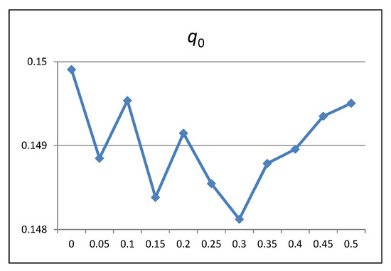
Figure 1.
Calibration of the probability of choosing the element with the highest score.
Figure 2a,b shows the results obtained for the evaporation rates. According to those, we set and . Since both are small values, the pheromone trails will be very persistent, especially in the case of local updates, which are performed more frequently than the global ones.
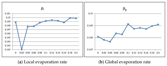
Figure 2.
Calibration of the evaporation rates.
Finally, we varied and . The results led us to set , meaning that at the start of the metaheuristic the weight of the greedy functions is 0.2, and .
5.2. Description of the Test Cases
The proposed ACO Algorithm has been tested on two realistic test cases with different characteristics: Haiti earthquake 2010 and Niger famine 2005.
The first test case is based on the earthquake that devastated Port-au-Prince, Haiti’s capital, and its metropolitan area in 2010. It was introduced in [29], and it is very appropriate to illustrate the problem, since many of the characteristics that define it are present here. It develops mainly in an urban environment, but the effects of the disaster produced a great uncertainty about the transitability of many streets. Besides, aid operations were carried out in an environment of insecurity, with frequent attacks to convoys.
The logistic map, illustrated in Figure 3, corresponds to the situation of the Port-au-Prince area fifteen days after the main earthquake. The network consists of 24 nodes and 84 arcs, corresponding to 42 two-way links. Nodes 1, 2 and 3 are supply nodes, with 60, 80 and 140 tons of humanitarian aid available, respectively. Nodes 10, 12, 13, 16, 17, 18, 20, 21 y 22 are demand nodes, with demands of 30, 40, 30, 30, 10, 30, 40, 20 y 20 tons of aid, respectively. Of these demand nodes, node 13 has special priority. The remaining 12 nodes are connection nodes and can be used to transship load.
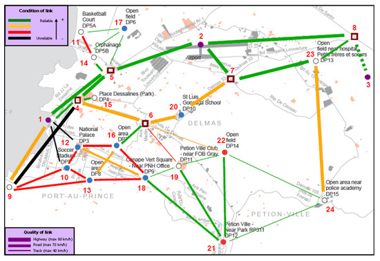
Figure 3.
Transport network at Port-au-Prince.
The links have been classified by their quality (according to the thickness of the line: the thicker the line, the higher the speed) and by their reliability (according to the color scale shown in the figure). The arcs also have different ransack probabilities.
To perform the distribution operations there are 300 vehicles, classified in three different types according to their velocities, costs and capacities. There are 70 large vehicles, 95 medium size vehicles, and 135 small vehicles, which can carry 3, 2 and 1 tons of aid, respectively. The vehicles are located at the supply nodes and at the connection nodes 4, 6 and 18. The purpose of the operation is to deliver 150 tons of aid among the demand nodes.
The data for the Haiti test case come from various documents available in January 2010: a logistic map provided by the United Nations Office for the Coordination of Humanitarian Affairs (OCHA) [44], a map reporting the satellite-identified IDP concentrations, road and bridge obstacles in central Port-au-Prince, Haiti, created by the United Nations Institute for Training and Research (UNITAR), and a map focused only on the Port-au-Prince road conditions created by the World Food Programme (WFP) Emergency Preparedness and Response [45].
The second test case, introduced in Vitoriano et al. [46], is based on the 2005 Niger food crisis. The logistic network (see Figure 4) consists of two supply nodes (Niamey and Gaya cities), two demand nodes (Agadez and Zinder), three connection nodes (Dosso, Tahoua and Maradi) and 11 two-way roads. There are a total of 376 vehicles available of three different types located at the supply and connection nodes to distribute 500 tons of humanitarian aid. The data for this test case come from the report of the real operation developed by the Spanish organization Fondo de Ayuda Humanitaria y de Emergencias de Farmamundi (FAHE) [47] and public websites such as Google Maps.
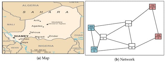
Figure 4.
Transport network at Niger.
Both test cases are explained in detail in [30] and their data are available on the website: www.mat.ucm.es/humlog.
5.3. Results
In this section we will compare and analyze the results obtained when applying the ACO Algorithm, proposed in this paper, and the GRASP Algorithm, introduced in [16], to the Haiti and Niger test cases. Furthermore, we compare as well the best solutions obtained by both algorithms with the optimal values for these test cases when they are available. These optimal values were obtained by solving to optimality relaxed flow models [28,29].
Firstly, we present the results obtained in the Haiti test case. Both algorithms—ACO and GRASP—have been executed ten times minimizing each objective independently and ten more times minimizing the aggregated function with equal weights for all attributes. The parameters of the algorithm were set according to the results of Section 5.1. A fixed computation time of 1500 s has been set for each of the 140 executions—two algorithms, seven objectives per algorithm and ten runs per objective.
Table 4 shows the computational results obtained with the ACO Algorithm and with the GRASP Algorithm in the Haiti test case. For each algorithm, the objective values of the best and the worst solutions among the ten executions are presented, as well as the average and the standard deviation of the objective values of the ten solutions. In this test case the operation time is given in minutes, the cost in dollars, and the security and the reliability in expected lost tons. We can see that the ACO Algorithm provides a better best solution when minimizing time, cost and security attributes, although for the cost the average is worse than with GRASP. For the reliability attribute, both algorithms provide the same best result, but this best is obtained in all GRASP executions—standard deviation is equal to zero—and only in two ACO executions. Both algorithms provide optimal solutions for the priority attribute in all executions and ACO performs worse than GRASP for the equity and for the aggregated function. The ACO algorithm provides around 10,000 feasible solutions on average while the GRASP algorithm provides 25,000. Nevertheless, this substancial difference does not translate into a proportional improvement in performance.
Table 4.
Results obtained with ten executions per objective of GRASP and ACO algorithms in Haiti earthquake 2010.
Table 5 shows the best values obtained among all tests performed during the experimentation—not only the ten executions of the previous table—in the Haiti test case, together with the optimal values for the attributes in which they are known. The optimal values for time and cost were obtained by using the static flow model described in [29], which although has some different assumptions, can serve as a reference for these two attributes that are measured in a very similar way. The ACO Algorithm provides the assumed optimal value for the time attribute and stays very close to the optimum for the cost, substantially improving the results obtained with the GRASP Algorithm. For the priority and the reliability attributes, both algorithms provide the same values, and almost the same for the security, whereas for the equity attribute, the ACO Algorithm performs worse. For the aggregated function, the GRASP Algorithm also works better, probably because of the higher influence of the equity attribute in the aggregated function, due to its tighter bound in comparison to the other attributes.
Table 5.
Best values obtained with several executions of GRASP and ACO algorithms in Haiti earthquake 2010.
Figure 5 depicts the itineraries of the best solutions found for the time and the cost attributes. The numbers on the arcs represent the amounts of aid transported by the vehicles traversing them (a “0” on an arc indicates that an empty convoy is traversing the arc). In the best solution for the time (Figure 5a), the three demand nodes farther from the supply nodes (18, 21 and 22) do not receive any aid and the distribution is mainly carried out by fast arcs, regardless of their dangerousness or reliability. The transportation is done by small and medium-sized vehicles, because they are faster than the large ones. When the cost attribute is optimized (Figure 5b), only a few arcs are used and the convoys consist mainly of large vehicles, giving a better cost-capacity ratio. In this solution three demand nodes, including the priority node (13), are not visited.
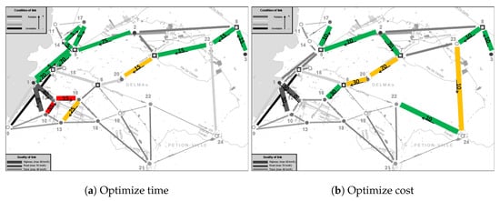
Figure 5.
Best itineraries optimizing time and cost in Haiti earthquake 2010.
Figure 6 shows the solution obtained when minimizing with equal weights. In this case, the ACO algorithm has been executed until 25,000 feasible solutions have been generated. This compromise solution provides reasonably good values for all attributes, as it can be observed in Table 6, all demand nodes receive some aid and, in particular, the priority node receives 26 out of 30 tons demanded.
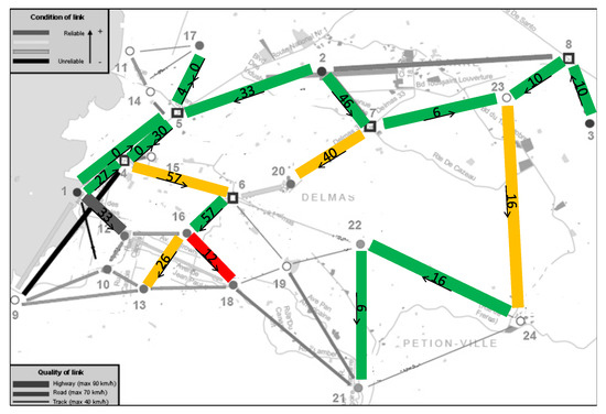
Figure 6.
Best itineraries optimizing in Haiti earthquake 2010.
Table 6.
Best objective values optimizing in Haiti earthquake 2010.
Finally, we summarize the results obtained in the Niger test case. As in the Haiti test case, GRASP and ACO have been executed ten times minimizing each objective independently and ten times minimizing the aggregated function, running 1500 s per execution. Again, Table 7 shows the objective values of the best and the worst solutions among the ten executions for each attribute, together with the average and the standard deviation of the objective values of the ten solutions. The operation time is given in hours, the cost in euros, and the security and the reliability in expected lost tons. Both algorithms provide optimal solutions for the equity and priority objectives in the ten executions. The ACO Algorithm performs slightly better than GRASP for the security and significantly better for the remaining attributes—time, cost and reliability—and also for the aggregated function. The best value obtained with ACO for the cost is only 1.6% higher than the assumed optimal value of the cost attribute, which is EUR 63,240.0, obtained using the static flow model [28]. ACO is significantly better for the cost, the time, the reliability and the aggregated function. Despite the higher speed of GRASP generating feasible solutions in this test case—9000 on average per execution with GRASP versus 6400 with ACO—ACO performance is much better than that of GRASP.
Table 7.
Results obtained with ten executions per objective of GRASP and ACO algorithms in Niger Famine 2005.
It is remarkable that the number of feasible solutions generated using the same computation time is lower in the Niger test case than in the Haiti test case, even though the logistic network is much smaller in the former. This is because there are other factors that influence the computation time as, for example, the structure of the network, the number and the location of the vehicles, the relation between the amount to be distributed and the total capacity of the vehicles, etc.
The proposed compromise solution for the Niger test case is shown in Table 8. All attribute values remain reasonably close to the best values obtained by optimizing each objective individually, except the value for the priority objective. This is partially due to the high confrontation between the equity and priority attributes. For optimizing the priority attribute, the node with the highest priority level (Zinder) should receive all the demanded aid, which would lead to an inequitable distribution.
Table 8.
Best objective values optimizing in Niger famine 2005.
In summary, the results obtained in both test cases show that the ACO Algorithm is able to obtain good solutions for all attributes when optimizing each of them individually, together with good compromise solutions as well. In particular, it provides the best known solutions for several attributes, such as the operation time in the Haiti test case or the reliability of the itineraries in the Niger test case. In addition, the computational effort required by the ACO algorithm is quite reasonable, making it suitable to solve realistic cases.
5.4. Managerial Insights
- The security issues related to the distribution of humanitarian aid, mainly focused on avoiding possible assaults to the vehicles performing the distribution operations in dangerous areas, are a key element in certain contexts, as for example war zones or extremely poor places. In these situations, it is frequently required that the vehicles involved are grouped forming convoys, as a protection mechanism and to allow escort details monitoring. This condition introduces significant additional difficulties into the last mile distribution models that must be properly addressed, but it makes the models more realistic and useful. The proposed metaheuristic algorithm can be used to obtain the precise distribution plan in an efficient way.
- In this work, two case studies, regarding an earthquake and a famine, a rapid and a slow onset disaster, respectively, have been considered. However, the proposed model and solution method can be applied to any kind of disaster, especially to the ones occurring in unsecure environments.
6. Concluding Remarks
This paper addresses a humanitarian last mile distribution problem in response to a disaster. The distribution must be done under unsecure conditions, so the vehicles must travel in convoys to try to prevent assaults. Furthermore, there is uncertainty about the state of the roads, that may have been damaged by the disaster. The proposed model is multimodal, multidepot, allows split deliveries and multiple trips and provides the individual itineraries of the vehicles. Besides, the model considers six performance criteria—time, cost, equity, priority, security and reliability—and is solved by a compromise programming approach.
The main contribution of this paper is the proposed methodology to solve the model. We develop an algorithm based on Ant Colony Optimization that considers several types of ants and pheromones. The methodology introduces the concept of effective pheromones to balance the elements of the provided solutions and to diversify the set of obtainable solutions. This methodology is especially appropriate to approach routing problems in which the vehicles are required to travel in convoys, but some of its most novel elements, as it is the case of the effective pheromones, could also be successfully applied to many other complex distribution and routing problems.
The algorithm is tested on two realistic case studies of public domain, and its performance is compared to that of the GRASP Algorithm, the only existing solution method in the literature. The ACO Algorithm performs well for all the objective functions tested in our experiments and provides, for both test cases considered, the best solutions obtained to date for several attributes. In comparison with the available solution method in the literature—the GRASP Algorithm—in the Haiti test case, both algorithms have their own strengths, but in the Niger test case, ACO clearly outperforms GRASP. The computation time required to obtain good solutions is reasonable in all cases, proving that the ACO Algorithm can be perfectly applied in an emergency context. Furthermore, GRASP and ACO algorithms actually complement each other and could even be used in combination in order to improve the quality of the final solutions provided to the decision makers.
One interesting future research line to continue this work comprises the development of a stochastic model in which the possibility of suffering assaults or finding blocked roads could be represented by random variables. Additionally, the design of simulation models to replicate real situations and test different solution strategies could also be worth considering.
Author Contributions
Conceptualization, J.M.F., M.T.O. and G.T.; Methodology, J.M.F., M.T.O. and G.T.; Software, J.M.F.; Validation, J.M.F., M.T.O. and G.T.; Formal analysis, J.M.F., M.T.O. and G.T.; Investigation, J.M.F., M.T.O. and G.T.; Data curation, J.M.F., M.T.O. and G.T.; Writing—original draft preparation, J.M.F.; Writing—review and editing, M.T.O. and G.T.; Visualization, J.M.F., M.T.O. and G.T.; Project administration, M.T.O. and G.T. All authors have read and agreed to the published version of the manuscript.
Funding
This research was funded by the European Commission grant H2020 MSCA-RISE 691161 (GEO-SAFE), the Government of Spain grant MTM2015-65803-R and the Government of Madrid, grant S2013/ICE-2845. The APC was funded by the European Commission grant H2020 MSCA-RISE 691161 (GEO-SAFE).
Conflicts of Interest
The authors declare no conflict of interest.
References
- Altay, N.; Green, W.G. OR/MS research in disaster operations management. Eur. J. Oper. Res. 2006, 175, 475–493. [Google Scholar] [CrossRef]
- Özdamar, L.; Ertem, M.A. Models, solutions and enabling technologies in humanitarian logistics. Eur. J. Oper. Res. 2015, 244, 55–65. [Google Scholar] [CrossRef]
- Tomasini, R.; van Wassenhove, L. Humanitarian Logistics; Palgrave Macmillan: London, UK, 2009. [Google Scholar]
- Vitoriano, B.; Montero, J.; Ruan, D. Decision Aid Models for Disaster Management and Emergencies; Atlantis Press: Paris, France, 2013. [Google Scholar]
- Pedraza-Martínez, A.J.; Van Wassenhove, L.N. Empirically grounded research in humanitarian operations management: The way forward. J. Oper. Manag. 2016, 45, 1–10. [Google Scholar] [CrossRef]
- Besiou, M.; Pedraza-Martínez, A.J.; Van Wassenhove, L.N. OR applied to humanitarian operations. Eur. J. Oper. Res. 2018, 269, 397–405. [Google Scholar] [CrossRef]
- Fiedrich, F.; Gehbauer, F.; Rickers, U. Optimized resource allocation for emergency response after earthquake disasters. Saf. Sci. 2000, 35, 41–57. [Google Scholar] [CrossRef]
- Viswanath, K.; Peeta, S. Multicommodity maximal covering network design problem for planning critical routes for earthquake response. Transp. Res. Rec. 2003, 1857, 1–10. [Google Scholar] [CrossRef]
- Kongsomsaksaku, S.; Yang, C.; Chen, A. Shelter location-allocation model for flood evacuation planning. J. East. Asia Soc. Transp. Stud. 2005, 6, 4237–4252. [Google Scholar]
- Barzinpour, F.; Saffarian, M.; Makoui, A.; Teimoury, E. Metaheuristic Algorithm for Solving Biobjective Possibility Planning Model of Location-Allocation in Disaster Relief Logistics. J. Appl. Math. 2014, 2014, 239868. [Google Scholar] [CrossRef][Green Version]
- Yi, W.; Özdamar, L. A dynamic logistics coordination model for evacuation and support in disaster response activities. Eur. J. Oper. Res. 2007, 179, 1177–1193. [Google Scholar] [CrossRef]
- Habib, M.S.; Sarkar, B. An Integrated Location-Allocation Model for Temporary Disaster Debris Management under an Uncertain Environment. Sustainability 2017, 9, 716. [Google Scholar] [CrossRef]
- Huang, M.; Smilowitz, K.; Balcik, B. Models for relief routing: Equity, efficiency and efficacy. Transp. Res. Part E Logist. Transp. Rev. 2012, 48, 2–18. [Google Scholar] [CrossRef]
- Holguín-Veras, J.; Pérez, N.; Jaller, M.; Van Wassenhove, L.; Aros-Vera, F. On the appropriate objective function for post-disaster humanitarian logistics models. J. Oper. Manag. 2013, 31, 262–280. [Google Scholar] [CrossRef]
- Gutjahr, W.J.; Nolz, P.C. Multicriteria optimization in humanitarian aid. Eur. J. Oper. Res. 2016, 252, 351–366. [Google Scholar] [CrossRef]
- Ferrer, J.M.; Ortuño, M.T.; Tirado, G. A GRASP metaheuristic for humanitarian aid distribution. J. Heuristics 2016, 22, 55–87. [Google Scholar] [CrossRef]
- Balcik, B.; Beamon, B.M.; Smilowitz, K. Last mile distribution in humanitarian relief. J. Intell. Transp. Syst. 2008, 12, 51–63. [Google Scholar] [CrossRef]
- Nolz, P.C.; Semet, F.; Doerner, K.F. Risk approaches for delivering disaster relief supplies. OR Spectrum 2011, 33, 543–569. [Google Scholar] [CrossRef]
- Lin, Y.H.; Batta, R.; Rogerson, P.A.; Blatt, A.; Flanigan, M. A logistics model for emergency supply of critical items in the aftermath of a disaster. Socio-Econ. Plan. Sci. 2012, 45, 132–145. [Google Scholar] [CrossRef]
- Bozorgi-Amiri, A.; Jabalameli, M.S.; Al-e Hashem, S.M.J.M. A multi-objective robust stochastic programming model for disaster relief logistics under uncertainty. OR Spectrum 2013, 35, 905–933. [Google Scholar] [CrossRef]
- Tirado, G.; Martín-Campo, F.J.; Vitoriano, B.; Ortuño, M.T. A lexicographical dynamic flow model for relief operations. Int. J. Comput. Int. Syst. 2014, 7, 45–57. [Google Scholar] [CrossRef]
- Huang, K.; Jiang, Y.; Yuan, Y.; Zhao, L. Modeling multiple humanitarian objectives in emergency response to large-scale disasters. Transp. Res. Part E Logist. Transp. Rev. 2015, 75, 1–17. [Google Scholar] [CrossRef]
- Ahmadi, M.; Seifi, A.; Tootooni, B. A humanitarian logistics model for disaster relief operation considering network failure and standard relief time: A case study on San Francisco district. Transp. Res. Part E Logist. Transp. Rev. 2015, 75, 145–163. [Google Scholar] [CrossRef]
- Zhou, Y.; Liu, J.; Zhang, Y.; Gan, X. A multi-objective evolutionary algorithm for multi-period dynamic emergency resource scheduling problems. Transp. Res. Part E Logist. Transp. Rev. 2017, 99, 77–95. [Google Scholar] [CrossRef]
- Maghfiroh, M.F.N.; Hanaoka, S. Last mile distribution in humanitarian logistics under stochastic and dynamic consideration. In Proceedings of the 2017 IEEE International Conference on Industrial Engineering and Engineering Management (IEEM), Singapore, 10–13 December 2017; pp. 1411–1415. [Google Scholar]
- Moreno, A.; Alem, D.; Ferreira, D.; Clark, A. An effective two-stage stochastic multi-trip location-transportation model with social concerns in relief supply chains. Eur. J. Oper. Res. 2018, 269, 1050–1071. [Google Scholar] [CrossRef]
- Habib, M.S.; Sarkar, B.; Tayyab, M.; Saleem, M.W.; Hussain, A.; Ullah, M.; Omair, M.; Iqbal, M.W. Large-scale disaster waste management under uncertain environment. J. Clean. Prod. 2019, 212, 200–222. [Google Scholar] [CrossRef]
- Ortuño, M.T.; Tirado, G.; Vitoriano, B. A lexicographical goal programming based decision support system for logistics of Humanitarian Aid. TOP 2011, 19, 464–479. [Google Scholar] [CrossRef]
- Vitoriano, B.; Ortuño, M.T.; Tirado, G.; Montero, J. A multi-criteria optimization model for humanitarian aid distribution. J. Glob. Optim. 2011, 51, 189–208. [Google Scholar] [CrossRef]
- Ferrer, J.M.; Martín-Campo, F.J.; Ortuño, M.T.; Pedraza-Martínez, A.J.; Tirado, G.; Vitoriano, B. Multi-criteria optimization for last mile distribution of disaster relief aid: Test cases and applications. Eur. J. Oper. Res. 2018, 269, 501–515. [Google Scholar] [CrossRef]
- Rizzoli, A.E.; Montemanni, R.; Lucibello, E.; Gambardella, L.M. Ant colony optimization for real-world vehicle routing problems. Ann. Oper. Res. 2007, 1, 135–151. [Google Scholar] [CrossRef]
- Yu, B.; Yang, Z.Z.; Xie, J.X. A parallel improved ant colony optimization for multi-depot vehicle routing problem. J. Oper. Res. Soc. 2011, 62, 183–188. [Google Scholar] [CrossRef]
- Zhang, L.Y.; Fei, T.; Zhang, X.; Li, Y.; Yi, J. Research about Immune Ant Colony Optimization in Emergency Logistics Transportation Route Choice. In Communications and Information Processing; Zhao, M., Sha, J., Eds.; Communications in Computer and Information Science; Springer: Berlin/Heidelberg, Germany, 2012; Volume 288, pp. 430–437. [Google Scholar]
- Hong, J.; Diabat, A.; Panicker, V.V.; Rajagopalan, S. A two-stage supply chain problem with fixed costs: An ant colony optimization approach. Int. J. Prod. Econ. 2018, 204, 214–226. [Google Scholar] [CrossRef]
- Yi, W.; Kumar, A. Ant colony optimization for disaster relief operations. Transp. Res. Part E Logist. Transp. Rev. 2007, 43, 660–672. [Google Scholar] [CrossRef]
- Saeidian, B.; Mesgari, M.S.; Pradhan, B.; Ghodousi, M. Optimized Location-Allocation of Earthquake Relief Centers Using PSO and ACO, Complemented by GIS, Clustering, and TOPSIS. ISPRS Int. J. Geo-Inf. 2018, 7, 292. [Google Scholar] [CrossRef]
- Cochrane, J.L.; Zeleny, M. Multiple Criteria Decision Making; University of South Carolina Press: Columbia, SC, USA, 1973. [Google Scholar]
- Dorigo, M.; Maniezzo, V.; Colorni, A. Ant system: Optimization by a colony of cooperating agents. IEEE Trans. Syst. Man Cybern. Part B Cybern. 1996, 26, 29–41. [Google Scholar] [CrossRef] [PubMed]
- Dorigo, M.; Blum, C. Ant colony optimization theory: A survey. Theor. Comput. Sci. 2005, 344, 243–278. [Google Scholar] [CrossRef]
- Zhao, N.; Wu, Z.; Zhao, Y.; Quan, T. Ant colony optimization algorithm with mutation mechanism and its applications. Expert Syst. Appl. 2010, 37, 4805–4810. [Google Scholar] [CrossRef]
- Chandra Mohan, B.; Baskaran, R. A survey: Ant Colony Optimization based recent research and implementation on several engineering domain. Expert Syst. Appl. 2012, 39, 4618–4627. [Google Scholar] [CrossRef]
- Dorigo, M.; Gambardella, L.M. Ant colony system: A cooperative learning approach to the traveling salesman problem. IEEE Trans. Evol. Comput. 1997, 1, 53–66. [Google Scholar] [CrossRef]
- Ford, L.R.; Fulkerson, D.R. Maximal flow through a network. Can. J. Math. 1956, 8, 399–404. [Google Scholar] [CrossRef]
- United Nations Office for the Coordination of Humanitarian Affairs (OCHA). Available online: https://www.unocha.org/ (accessed on 17 March 2020).
- World Food Programme (WFP) Emergency Preparedness and Response. Available online: https://www.wfp.org/emergency-preparedness-and-response (accessed on 17 March 2020).
- Vitoriano, B.; Ortuño, M.T.; Tirado, G. HADS, a goal programming-based humanitarian aid distribution system. J. Multi-Crit. Decis. Anal. 2009, 16, 55–64. [Google Scholar] [CrossRef]
- Fondo de Ayuda Humanitaria y de Emergencias de Farmamundi (FAHE). Memoria. 2005. Available online: http://www.farmaceuticosmundi.org/farmamundi/descargas/pdf/memoria_2005_fahe.pdf (accessed on 17 March 2020).
© 2020 by the authors. Licensee MDPI, Basel, Switzerland. This article is an open access article distributed under the terms and conditions of the Creative Commons Attribution (CC BY) license (http://creativecommons.org/licenses/by/4.0/).