Article

Designing Developable C-Bézier Surface with Shape Parameters

1
School of Mathematical and Physical Sciences, Dalian University of Technology, Panjin 124221, China
2
School of Mathematical Sciences, Dalian University of Technology, Dalian 116024, China
*
Author to whom correspondence should be addressed.
Mathematics 2020, 8(3), 402; https://doi.org/10.3390/math8030402
Submission received: 16 February 2020 / Revised: 8 March 2020 / Accepted: 9 March 2020 / Published: 11 March 2020
(This article belongs to the Special Issue Modern Geometric Modeling: Theory and Applications)

Abstract

:
Developable surface plays an important role in geometric design, architectural design, and manufacturing of material. Bézier curve and surface are the main tools in the modeling of curve and surface. Since polynomial representations can not express conics exactly and have few shape handles, one may want to use rational Bézier curves and surfaces whose weights control the shape. If we vary a weight of rational Bézier curve or surface, then all of the rational basis functions will be changed. The derivation and integration of the rational curve will yield a high degree curve, which means that the shape of rational Bézier curve and surface is not easy to control. To solve this problem of shape controlling for a developable surface, we construct C-Bézier developable surfaces with some parameters using a dual geometric method. This yields properties similar to Bézier surfaces so that it is easy to design. Since C-Bézier basis functions have only two parameters in every basis, we can control the shape of the surface locally. Moreover, we derive the conditions for C-Bézier developable surface interpolating a geodesic.

1. Introduction

Developable surface is a special ruled surface with vanishing Gaussian curvature. They can be unfolded or developed onto a plane without stretching and tearing. Based on these properties, they have many applications in computer aided geometric design (CAGD), especially for the designing the surface of some products, such as shoes, hat, ship hull and car body, etc. Therefore, the design of developable surface is of considerable importance to plate-metal-based and sheet-metal industries. A developable surface is either a cylindrical surface, a conical surface, or a tangent surface.
There are mainly methods to study developable surfaces in current computer aided design (CAD)/computer aided manufacturing (CAM) system. One method is point geometry. We can refer to the papers [1,2,3,4,5,6,7]. Aumann [1] proposed the conditions to construct a developable Bézier surface with two boundary curves that are restricted in parallel planes. Lang and R o ¨ schel [2] studied the necessary conditions of a rational developable Bézier surface by characterizing the weights and the control nets. The main drawback of this method is the production of coupled equations that is very difficult for the designing of developable surfaces in a CAD system. Another approach is projective geometry, which is proposed by Pottmann and Farin [4]. In this viewpoint, a developable surface can be represented as a curve in projective space. Because of the curve scheme, the nonlinear characterization equations can be avoided. Bodduluri and Ravani [7] developed a new representation for developable surfaces by using the concept of duality between points and planes in projective space. Moreover, Zhao and Wang [8] and Li et al. [9] constructed the developable surface to interpolate geodesic and line of curvature, respectively.
The above approaches were almost confined on Bézier or B-spline surfaces. It is uncontrollable and has trouble adjusting the shape of the developable surface because of a few degrees of freedom. These disadvantages make them difficult to meet the needs of the practice engineering. Of course, we can consider using a rational Bézier surface. However, just as mentioned by Farin [10] and Piegl [11], the higher power of a rational model can induce several drawbacks:
  • Rational curves and surfaces have weights for each control point. In general, the selection of the weight is not clear. Thus, the author in [12] concluded that “this added freedom of weights is potentially more a nuisance than a real help”.
  • We know that the derivative of a degree n polynomial curve is a curve of degree n 1 ; this means that differential yields a simpler curve. However, the derivative of a degree n rational curve is a rational curve of degree 2 n . Thus, the derivative yields a curve with a high degree. If we repeat differentiation, we will get a curve of a high degree. It may not be dealt with in the CAD system.
  • The rational model can not encompass transcendental curves, such as cycloid and helix. The curves are very important in technical application.
To overcome these shortcomings, some researchers introduced the curve and surface with parameter. Zhang [13] proposed C-curves, which are an extension of cubic curves. These new curves depend on a parameter; when the parameter tends to 0, they degenerated to cubic curves. Following this paper, Zhang introduced C-B splines in [14]. He gave a new reparametrized form of C-B splines, and derived the third form that has different parameters. By using the same techniques of C-B splines, Zhang discussed two other forms of C-Bézier curves and a reformed formula for the subdivisions in [15]. Under these new forms, C-Bézier curves can make the processes of the normal cases and the limiting case with precise results unified. Han, Ma, and Huang [16] proposed a class of polynomial basis functions with n adjustable shape parameters. The authors constructed quasi-Bézier curves and surfaces, which can be flexibly controlled by suitably modifying the values of the shape parameters. Zhu and Han [17] constructed four new cubic rational Bernstein-like basis functions with two parameters by using the blossom method. These basis functions can form a normalized B-basis. They analyzed their good properties. Zhu, Han, and Liu [18] also studied four new α β -Bernstein-like basis functions with two exponential shape parameters. These basis functions include the cubic Said–Ball basis functions and cubic Bernstein basis functions. They developed a new corner cutting algorithm. Zhou et al. [19] constructed developable surfaces of C-Bézier basis functions with one shape parameter. Hu et al. [20] studied λ Bézier developable surface and their properties. They can control the shape of the developable surface without altering the position of the control points. However, there is only one parameter, which is limited to adjust the developable surface. Hu et al. [21] proposed a novel method for constructing 1 × 3 developable H-Bézier surfaces with three parameters. In recent years, several trigonometric splines have been studied. In [22], the authors constructed the cubic trigonometric polynomial spline curve of G 3 continuity, which can be G 5 continuity under special conditions. Yang and Liang [23] presented algebraic-trigonometric blended spline curves which can represent some transcendental curves.
In this paper, in order to solve the shape handling problem of the developable surface, we introduce new basis functions with n parameters by integral. In addition to some similar properties of Bézier basis, the new basis functions have better handling because of the parameters. We analyze the good properties of the new basis functions and prove them. Due to the merits of the new basis, we can extend them to curves and surfaces. Considering the application of the developable surface in designing of the car body, airplane skin, and shoes, we construct developable surfaces under the new basis by enveloping developable and tangent of spine curve. The shape of the surface can be easily controlled dual to the parameters, so it will provide more convenience for designing the apparent surface of some products. The rest of the paper is organized as follows. Section 2 gives generalized C-Bézier basis functions with n parameters and its properties. In Section 3, we construct the developable surface by two approaches. One is considered as the envelope of the one-parameter pencils of tangent planes. The other is that we express the developable surface as the tangent surface of regression line. We only need to adjust the shape of the surface by shape parameters without moving the control points. Moreover, we give the concrete expression of n-parameters C-Bézier developable surface interpolating geodesic. We do the examples on a 1.8 GHz PC by the software Maple, and the examples show the method is effective.

2. C-Bézier Curve with n -Parameters

2.1. C-Bézier Basis Functions with n-Parameters

Zhang [13,14] investigated cubic C-curves and C-surfaces with one parameter α in the space span { 1 , t , cos t , sin t } . Chen [24] constructed a new C-Bézier basis with degree n for the span { 1 , t , t 2 , , t n 2 , sin t , cos t } by an integral approach. These bases share the same properties as the Bernstein basis when the parameter α 0 . Because such basis has only one parameter, there is a limit for adjusting the shape of the surface. In order to control the surface more flexibly, we construct a new basis function with n parameters. First, we choose the original functions as
u 0 , 1 ( t ; α ) = sin α ( 1 t ) sin α , u 1 , 1 ( t ; α ) = sin α t sin α ,
where α ( 0 , π ) , t [ 0 , 1 ] . Then, we can define
Definition 1.
C-Bézier basis functions with n parameters
u 0 , n ( t ; α 1 ) = 1 0 t δ 0 , n 1 u 0 , n 1 ( x ; α 1 ) d x , u i , n ( t ; α i , α i + 1 ) = 0 t [ δ i 1 , n 1 u i 1 , n 1 ( x ; α i ) δ i , n 1 u i , n 1 ( x ; α i + 1 ) ] d x , u n , n ( t ; α n ) = 0 t δ n 1 , n 1 u n 1 , n 1 ( x ; α n ) d x ,
where u i , n 1 ( x ; α i + 1 ) = u i , n 1 ( x ; α i + 1 , α i + 1 ) , δ i , n 1 = ( 0 1 u i , n 1 ( t ; α i + 1 ) d t ) 1 , i = 0 , 1 , , n 1 , t [ 0 , 1 ] . If n = 2 , α 2 ( 0 , π ] , if n 3 , α i ( 0 , 2 π ] .
According to Definition 1, we can compute the quadratic C-Bézier basis.
u 0 , 2 ( t ; α 1 ) = 1 0 t δ 0 , 1 u 0 , 1 ( x ; α 1 ) d x = 1 cos α 1 ( 1 t ) cos α 1 1 cos α 1 , u 1 , 2 ( t ; α 1 , α 2 ) = 0 t ( δ 0 , 1 u 0 , 1 ( x ; α 1 ) δ 1 , 1 u 1 , 1 ( x ; α 2 ) ) d x = cos α 1 ( 1 t ) cos α 1 1 cos α 1 1 cos α 2 t 1 cos α 2 , u 2 , 2 ( t ; α 2 ) = 0 t δ 1 , 1 u 1 , 1 ( x ; α 2 ) d x = 1 cos α 2 t 1 cos α 2 .
Figure 1 shows the basis functions with different parameters.
In the same manner, the cubic basis functions can be expressed as follows:
u 0 , 3 ( t ; α 1 ) = sin α 1 ( 1 t ) α 1 ( 1 t ) α 1 sin α 1 , u 1 , 3 ( t ; α 1 , α 2 ) = sin α 1 ( 1 t ) + α 1 t sin α 1 α 1 sin α 1 + ( 1 M 2 ) sin α 2 t + K 2 M 2 cos α 2 t ( 1 M 2 ) α 2 t K 2 M 2 α 2 sin α 2 , u 2 , 3 ( t ; α 2 , α 3 ) = ( 1 M 2 ) sin α 2 t + K 2 M 2 cos α 2 t ( 1 M 2 ) α 2 t K 2 M 2 α 2 sin α 2 α 3 t sin α 3 t α 3 sin α 3 , u 3 , 3 ( t ; α 3 ) = α 3 t sin α 3 t α 3 sin α 3 ,
where K 2 = α 2 sin α 2 1 cos α 2 , M 2 = 1 , α 2 = π ; sin α 2 ( 1 cos α 2 ) 2 sin α 2 α 2 α 2 cos α 2 , 0 < α 2 < π . The basis functions are shown in Figure 2.
The C-Bézier basis functions with parameters have the following properties.
Property 1.
The basis is normalized that is
u 0 , n ( t ; α 1 ) + i = 1 n 1 u i , n ( t ; α i , α i + 1 ) + u n , n ( t ; α n ) = 1 .
Proof. 
From Definition 1, it is obvious that the basis is normalized. □
Property 2.
At the endpoints, when n 2 , the basis satisfies
(a). 
u 0 , n ( 0 ; α 1 ) = u n , n ( 1 ; α n ) = 1 ;
(b). 
u i , n ( j ) ( 0 ; α i , α i + 1 ) = u i , n ( k ) ( 1 ; α i , α i + 1 ) = 0 , j = 0 , 1 , , i 1 ; k = 0 , 1 , , n i 1 ;
(c). 
u i , n ( i ) ( 0 ; α i , α i + 1 ) = δ i 1 , n 1 ( α i ) δ i 2 , n 2 ( α i ) δ 0 , n i ( α i ) , i = 1 , 2 , , n , δ 0 , 0 = α sin α .
Proof. 
(a).
By Definition 1,
u 0 , n ( 0 ; α 1 ) = 1 0 0 δ 0 , n 1 u 0 , n 1 ( x ; α 1 ) d x = 1 ; u n , n ( 1 ; α n ) = 0 1 δ n 1 , n 1 u n 1 , n 1 ( x ; α n ) d x = δ n 1 , n 1 0 1 u n 1 , n 1 ( x ; α n ) d x = 0 1 u n 1 , n 1 ( x ; α n ) d x 0 1 u n 1 , n 1 ( x ; α n ) d x = 1 .
(b).
We prove this property by induction on n. When n = 2 , we get u 1 , 2 ( 0 ; α 1 , α 2 ) = u 1 , 2 ( 1 ; α 1 , α 2 ) = 0 . Assume ( b ) holds on n 1 , that is,
u i , n 1 ( j ) ( 0 ; α i , α i + 1 ) = u i , n 1 ( k ) ( 1 ; α i , α i + 1 ) = 0 , j = 0 , , i 1 , k = 0 , , n i 2 .
Then, for n, we have
u i , n ( j ) ( 0 ; α i , α i + 1 ) = δ i 1 , n 1 u i 1 , n 1 ( j 1 ) ( 0 ; α i 1 , α i ) δ i , n 1 u i , n 1 ( j ) ( 0 ; α i , α i + 1 ) , u i , n ( k ) ( 1 ; α i , α i + 1 ) = δ i 1 , n 1 u i 1 , n 1 ( k 1 ) ( 1 ; α i 1 , α i ) δ i , n 1 u i , n 1 ( k ) ( 1 ; α i , α i + 1 ) .
According to Formula (2), it is easy to get
u i , n ( j ) ( 0 ; α i , α i + 1 ) = u i , n ( k ) ( 1 ; α i , α i + 1 ) = 0 , j = 0 , , i 1 , k = 0 , , n i 1 .
(c).
We prove this property by induction on n too. When n = 2 , we have
u 1 , 2 ( 0 ; α 1 , α 2 ) = α 1 sin α 1 1 cos α 1 = δ 0 , 1 ( α 1 ) , u 2 , 2 ( 0 ; α 2 ) = α 2 2 1 cos α 2 = δ 1 , 1 ( α 2 ) δ 0 , 0 ( α 2 ) .
Assume it holds for n 1 , that is, u i , n 1 ( i ) ( 0 ; α i , α i + 1 ) = δ i 1 , n 2 ( α i ) δ i 2 , n 3 ( α i ) δ 0 , n i 1 ( α i ) . On the left part of this equation, when we let t = 0 , the term including α i + 1 is zero. Therefore, the right side of the equation only has parameter α i . Then, we have
u i , n ( i ) ( 0 ; α i , α i + 1 ) = ( u i , n ) ( i 1 ) ( 0 ; α i , α i + 1 ) = ( δ i 1 , n 1 u i 1 , n 1 ( t ; α i , α i + 1 ) δ i , n 1 u i , n 1 ( t ; α i , α i + 1 ) ) ( i 1 ) t = 0
According to ( b ) , u i , n 1 ( t ; α i , α i + 1 ) ) ( i 1 ) t = 0 = 0 . Therefore,
u i , n ( i ) ( 0 ; α i , α i + 1 ) = δ i 1 , n 1 u i 1 , n 1 ( i 1 ) ( 0 ; α i , α i + 1 ) = δ i 1 , n 1 ( α i ) δ i 2 , n 2 ( α i ) δ i 3 , n 3 ( α i ) δ 0 , n i ( α i ) .
Property 3.
Linear independence.
Proof. 
Assume
a 0 u 0 , n ( t ; α 1 ) + i = 1 n 1 a i u i , n ( t ; α i , α i + 1 ) + a n u i , n ( t ; α n ) = 0 .
Then, by Property 2, we get
a 0 u 0 , n ( 0 ; α 1 ) + a 1 u 1 , n ( 0 ; α 1 , α 2 ) + + a n u n , n ( 0 ; α n ) = a 0 = 0
for t = 0 . Then, differential Equation ( 3 ) , according to Property 2, we have
a 1 δ 0 , n 1 ( α 1 ) = 0 ,
so a 1 = 0 . Similar to the above, we can differentiate Equation ( 3 ) n times, then we get a i = 0 , i = 2 , , n . This means that the functions u 0 , n ( t ; α 1 ) , { u i , n ( t ; α i , α i + 1 ) } i = 1 n 1 , u n , n ( t ; α n ) are linear independent. □
Property 4.
When n 3 , the basis functions u 0 , n ( t ; α 1 ) , { u i , n ( t ; α i , α i + 1 ) } i = 1 n 1 , u n , n ( t ; α n ) are positive.
Proof. 
For arbitrary f s p a n { sin α t , cos α t , t n 2 , , t , 1 } , assume f ( t ) = a sin α t + b cos α t + i = 0 n 2 t i has n + 2 roots in [ 0 , 1 ] . According to Rolle’s Theorem, f ( n 1 ) ( t ) has three roots in [ 0 , 1 ] . By computing, f ( n 1 ) ( t ) = A sin α t + B cos α t = C sin ( α t + φ ) , A , B , C , φ are constants. C sin ( α t + φ ) has two roots at most in [ 0 , 1 ] ; this is in contradiction with the assumption. Therefore, f ( t ) has n + 1 roots at most in [ 0 , 1 ] .
From the above theory, the basis u 0 , n ( t ; α 1 ) , { u i , n ( t ; α i , α i + 1 ) } i = 1 n 1 , u n , n ( t ; α n ) has n + 1 roots at most in [ 0 , 1 ] . By Property 2, 0 is i multiple root and 1 is n i multiple root:
u 0 , n ( t ; α 1 ) = j = 0 i u 0 , n ( j ) ( 0 ; α 1 ) t j j ! + o ( t j ) = u 0 , n ( 0 ; α 1 ) t i i ! + o ( t i ) , u i , n ( t ; α i , α i + 1 ) = j = 0 i u i , n ( j ) ( 0 ) t j j ! + o ( t j ) = u i , n ( i ) ( 0 ) t i i ! + o ( t i ) , 1 i n 1 , u n , n ( t ; α n ) = j = 0 i u n , n ( j ) ( 0 ; α n ) t j j ! + o ( t j ) = u n , n ( 0 ; α n ) t i i ! + o ( t i ) .
When n = 3 ,
u 1 , 3 ( 0 ; α 1 , α 2 ) = δ 0 , 2 ( α 1 ) = α 1 ( 1 cos α 1 ) α 1 sin α 1 > 0 , ( α 1 ( 0 , π ] ) ,
u 2 , 3 ( 0 ; α 2 , α 3 ) = δ 1 , 2 ( α 2 ) δ 0 , 1 ( α 2 ) = α 2 2 sin α 2 2 sin α 2 α 2 cos α 2 α 2 = α 2 2 sin α 2 α 2 2 cos α 2 2 ( sin α 2 2 α 2 2 cos α 2 2 ) .
If α 2 ( 0 , π ] , that is, α 2 2 ( 0 , π 2 ] . Then, sin α 2 > 0 , cos α 2 2 > 0 , sin α 2 2 α 2 2 cos α 2 2 > 0 , we get u 2 , 3 ( 0 ; α 2 , α 3 ) > 0 . For α 2 ( π , 2 π ] , sin α 2 < 0 , cos α 2 2 < 0 , sin α 2 2 α 2 2 cos α 2 2 > 0 , then u 2 , 3 ( 0 ; α 2 , α 3 ) > 0 .
u 3 , 3 ( 3 ) ( 0 ; α 3 ) = δ 2 , 2 δ 1 , 1 δ 0 , 0 = α 3 3 α 3 sin α 3 > 0 .
Therefore, u i , 3 ( i ) ( 0 ; α 3 ) > 0 , there exists δ > 0 , when t ( 0 , δ ) , u i , 3 ( t ; α 3 ) > 0 , while t ( 0 , δ ) , u i , 3 ( 1 t ; α 3 ) > 0 . If there exists t * ( 0 , 1 ) making u i , 3 ( t * ; α 3 ) < 0 , then u i , 3 ( t ; α 3 ) has two roots at least in ( 0 , 1 ) . In this case, u i , 3 ( t ; α 3 ) has five roots at least in [ 0 , 1 ] , it is a contradiction with the consumption that the basis u 0 , n ( t ; α 1 ) , { u i , n ( t ; α i , α i + 1 ) } i = 1 n 1 , u n , n ( t ; α n ) has n + 1 roots at most in [ 0 , 1 ] . Thus, u i , 3 ( t ; α 3 ) > 0 .
Assume 3 < n k 1 , u i , n ( t ; α i , α i + 1 ) > 0 , then δ i 1 , k 1 δ i 2 , k 2 , δ 0 , k 1 > 0 , that is, u i , k ( i ) ( 0 ; α i , α i + 1 ) > 0 . When n = k , u i , k ( t ; α i , α i + 1 ) is positive in a small enough right domain of 0 and a left domain of 1. If t * ( 0 , 1 ) makes u i , k ( t * ; α i , α i + 1 ) < 0 , then u i , k ( t ; α i , α i + 1 ) has at least two roots in ( 0 , 1 ) . Therefore, it has k + 2 roots at least in [ 0 , 1 ] , which is impossible. Consequently, u i , k ( t ) > 0 . □

2.2. C-Bézier Curve with n-Parameters

Definition 2.
Given n + 1 points P i R 3 ( i = 0 , , n ) , the parametric curve
P ( t ; α 1 , , α n ) = P 0 u 0 , n ( t ; α 1 ) + i = 1 n 1 P i u i , n ( t ; α i , α i + 1 ) + P n u n , n ( t ; α n ) , 0 t 1
is called C-Bézier curve of degree n with n-parameters, where P i are control points, α i are shape parameters.
Example 1.
By Definition 2 and cubic C-Bézier basis functions ( 1 ) , the cubic C-Bézier curve is given by
P ( t ) = P 0 u 0 , 3 ( t , α 1 ) + P 1 u 1 , 3 ( t ; α 1 , α 2 ) + P 2 u 2 , 3 ( t ; α 2 , α 3 ) + P 3 u 3 , 3 ( t ; α 3 ) ,
where t [ 0 , 1 ] , α i ( 0 , 2 π ] , i = 1 , 2 , 3 . Figure 3show cubic C-Bézier curves with different parameters.
By Example 1, we can note that such parametric curve construction can be potentially applied to extend linear opinion speading to multidimensional parametric spaces with embedded structural dynamics. See [25].
By the properties of C-Bézier basis functions and Definition 2, we have the following basic properties of C-Bézier curve with n-parameters.
Property 5.
Convex hull property. The entire C-Bézier curve with n-parameters must lie inside the convex hull of its control points.
Proof. 
By Properties 1 and 4, the basis functions u 0 , n ( t ; α 1 ) , { u i , n ( t ; α i , α i + 1 ) } i = 1 n 1 , u n , n ( t ; α n ) are positive and normalized. Therefore, for a given t, the C-Bézier curve P ( t ; α 1 , , α n ) is weighted average of the control points P i . That is, the curve P ( t ; α 1 , , α n ) lies in the convex hull formed by its control points. □
Property 6.
Endpoints’ interpolation and derivatives.
(a). 
P ( 0 ; α 1 , , α n ) = P 0 , P ( 1 ; α 1 , , α n ) = P n ;
(b). 
P ( j ) ( 0 ; α 1 , , α j + 1 ) = P 0 u 0 , n ( j ) ( 0 ; α 1 ) + i = 1 j P i u i , n ( j ) ( 0 ; α i , α i + 1 ) ;
(c). 
P ( j ) ( 1 ) = i = n j n 1 P i u i , n ( j ) ( 1 ; α i , α i + 1 ) + P n u n , n ( j ) ( 1 ; α n ) .
Proof. 
(a).
Let t = 0 ; then, Equation ( 4 ) is
P ( 0 ; α 1 , , α n ) = P 0 u 0 , n ( 0 ; α 1 , , α n ) + i = 1 n 1 P i u i , n ( 0 ; α i , α i + 1 ) + P n u n , n ( 0 ; α n ) .
By Property 2 ( a ) and 2 ( b ) , we have u 0 , n ( 0 ; α 1 ) = 1 , u i , n ( 0 ; α i , α i + 1 ) = 0 , u n , n ( 0 ; α n ) = 0 , then P ( 0 ; α 1 , , α n ) = P 0 . In the similar way, P ( 1 ; α 1 , , α n ) = P n .
(b).
When t = 0 ,
P ( j ) ( 0 ; α 1 , , α n ) = P 0 u 0 , n ( j ) ( 0 ; α 1 ) + i = 1 n 1 P i u i , n ( j ) ( 0 ; α i , α i + 1 ) + P n u n , n ( j ) ( 0 ; α n ) .
According to Property ( 2 ) ( b ) , u i , n ( j ) ( 0 ; α i , α i + 1 ) = 0 ( i = j + 1 , , n 1 ) , u n , n ( j ) ( 0 ; α n ) = 0 , so we have
P ( j ) ( 0 ; α 1 , , α j + 1 ) = P 0 u 0 , n ( j ) ( 0 ; α 1 ) + i = 1 j P i u i , n ( j ) ( 0 ; α i , α i + 1 ) .
(c).
By using the above method, we can prove conclusion ( c ) , so here we omit the process of the proof.
Property 7.
Differentiation property. The derivative P ( t ) of a degree n is a degree n 1 C-Bézier curve with ( n 1 ) -parameters, which can be expressed as
P ( t ) = i = 0 n 1 δ i , n 1 ( P i + 1 P i ) u i , n 1 ( t ; α i + 1 ) .
Proof. 
By differentiating Equation ( 4 ) , we get
P ( t ; α 1 , , α n ) = P 0 u 0 , n ( t ; α 1 ) + i = 1 n 1 P i u i , n ( t ; α i , α i + 1 ) + P n u n , n ( t ; α n ) .
We substitute the expression of the basis functions given in Definition 1; then,
P ( t ; α 1 , , α n ) = P 0 δ 0 , n 1 u 0 , n 1 ( t ; α 1 ) + P 1 ( δ 0 , n 1 u 0 , n 1 ( t ; α 1 ) δ 1 , n 1 u 1 , n 1 ( t ; α 2 ) ) + P 2 ( δ 1 , n 1 u 1 , n 1 ( t ; α 2 ) δ 2 , n 1 u 2 , n 1 ( t ; α 3 ) ) + + P n 1 ( δ n 2 , n 1 u n 2 , n 1 ( t ; α n 1 ) δ n 1 , n 1 u n 1 , n 1 ( t ; α n ) ) + P n δ n 1 , n 1 u n 1 , n 1 ( t ; α n ) = ( P 1 P 0 ) δ 0 , n 1 u 0 , n 1 ( t ; α 1 ) + + ( P n P n 1 ) δ n 1 , n 1 u n 1 , n 1 ( t ; α n ) = i = 0 n 1 δ i , n 1 ( P i + 1 P i ) u i , n 1 ( t ; α i + 1 ) .
The conclusion is proved. □

3. Developable Surface from Cubic C-Bézier Curve with Three Parameters

In this section, based on the C-Bézier basis functions and cubic C-Bézier curve defined in the last section, we propose two methods to design the developable surface with three parameters due to the following Definition 3.
Definition 3
([26]). Two planes in a plane family { t } intersect a line called the characteristic line. Three planes in a plane family { t } intersect a point called characteristic point.

3.1. 1 × 3 Enveloping Developable C-Bézier Surface
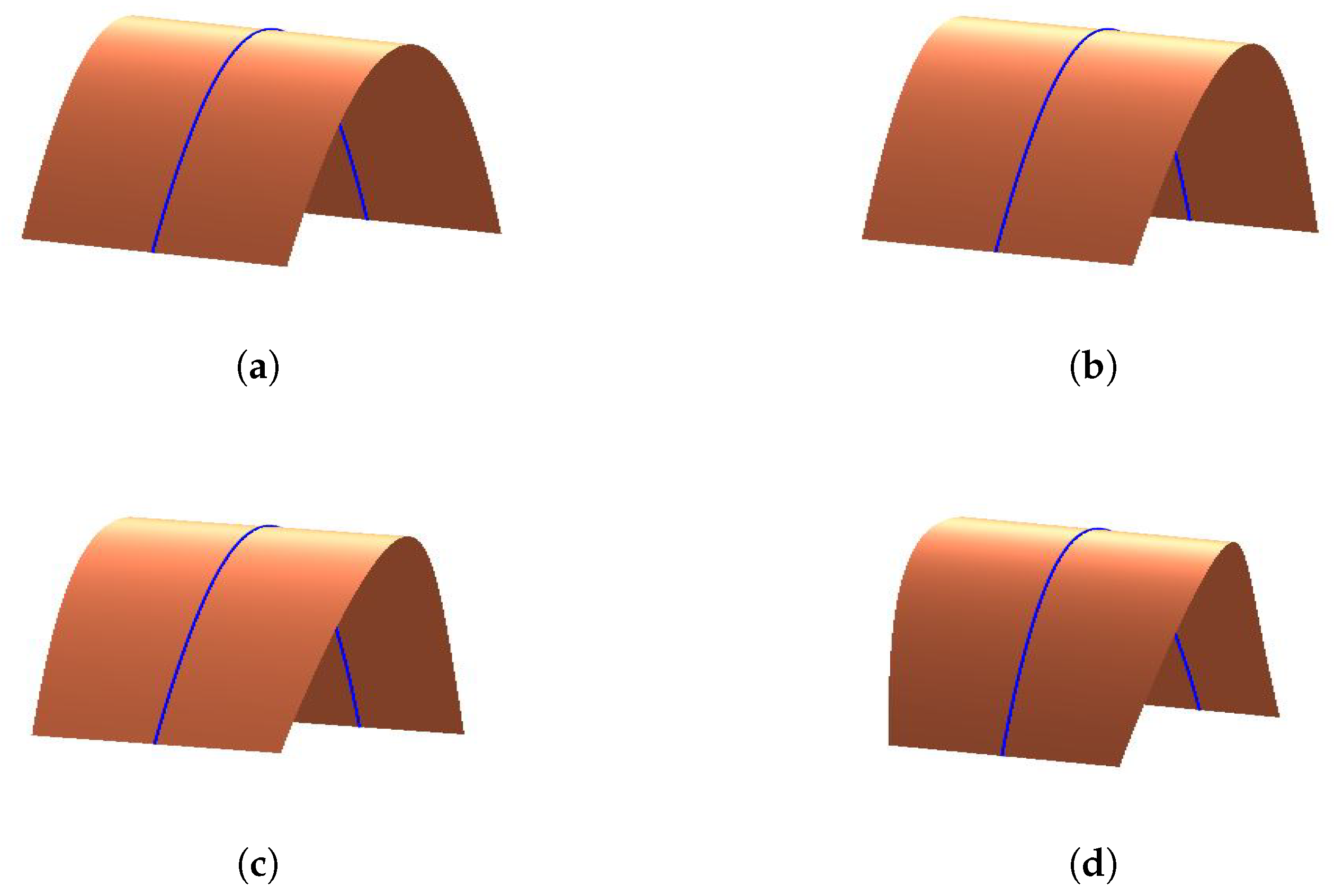
We mainly based on the theory that the dual element of point is plane, and the dual element of the line is a line in three-dimensional projective space. In the expression ( 5 ) , we substitute the control points P i ( i = 0 , 1 , 2 , 3 ) with control planes i ( i = 0 , 1 , 2 , 3 ) . Assume the coordinates of planes i ( i = 0 , 1 , 2 , 3 ) are Q i = ( a i , b i , c i , d i ) ( i = 0 , 1 , 2 , 3 ) ; then, we can get the single-parameter family of planes
{ t } : X ( t ; α 1 , α 2 , α 3 ) = ( x 0 ( t ) , x 1 ( t ) , x 2 ( t ) , x 3 ( t ) ) = Q 0 u 0 , 3 ( t , α 1 ) + Q 1 u 1 , 3 ( t , α 1 , α 2 ) + Q 2 u 2 , 3 ( t , α 2 , α 3 ) + Q 3 u 3 , 3 ( t , α 3 ) .
That is,
a 0 u 0 , 3 ( t , α 1 ) + a 1 u 1 , 3 ( t , α 1 , α 2 ) + a 2 u 2 , 3 ( t ; α 2 , α 3 ) + a 3 u 3 , 3 ( t ; α 3 ) = x 0 ( t ) , b 0 u 0 , 3 ( t , α 1 ) + b 1 u 1 , 3 ( t , α 1 , α 2 ) + b 2 u 2 , 3 ( t ; α 2 , α 3 ) + b 3 u 3 , 3 ( t ; α 3 ) = x 1 ( t ) , c 0 u 0 , 3 ( t , α 1 ) + c 1 u 1 , 3 ( t , α 1 , α 2 ) + c 2 u 2 , 3 ( t ; α 2 , α 3 ) + c 3 u 3 , 3 ( t ; α 3 ) = x 2 ( t ) , d 0 u 0 , 3 ( t , α 1 ) + d 1 u 1 , 3 ( t , α 1 , α 2 ) + d 2 u 2 , 3 ( t ; α 2 , α 3 ) + d 3 u 3 , 3 ( t ; α 3 ) = x 3 ( t ) .
According to the conditions of developable surface, the envelope of the a single-parameter family of planes is a developable surface. The plane at any of value t can be expressed as
x 0 ( t ) x + x 1 ( t ) y + x 2 ( t ) z = x 3 ( t ) .
Differential Equation ( 7 ) , that is,
x 0 ( t ) x + x 1 ( t ) y + x 2 ( t ) z = x 3 ( t ) .
By Definition 3, the intersecting line of the two planes ( 7 ) and ( 8 ) is the generator of the developable surface. We use L ( t ) = L ( s ( t ) , r ( t ) ) , which represents the generator, where
s ( t ) = ( x 0 ( t ) , x 1 ( t ) , x 2 ( t ) ) × ( x 0 ( t ) , x 1 ( t ) , x 2 ( t ) ) = ( x 1 ( t ) x 2 ( t ) x 2 ( t ) x 1 ( t ) , x 0 ( t ) x 2 ( t ) x 0 ( t ) x 2 ( t ) , x 0 ( t ) x 1 ( t ) x 1 ( t ) x 0 ( t ) )
is the directional vector of L ( t ) :
r ( t ) = x 3 ( t ) ( x 0 ( t ) , x 1 ( t ) , x 2 ( t ) ) x 3 ( t ) ( x 0 ( t ) , x 1 ( t ) , x 2 ( t ) ) = ( x 0 ( t ) x 3 ( t ) x 3 ( t ) x 0 ( t ) , x 1 ( t ) x 3 ( t ) x 1 ( t ) x 3 ( t ) , x 2 ( t ) x 3 ( t ) x 3 ( t ) x 2 ( t ) ) .
Assume P = ( x , y , z ) is the point, closest to the origin O ; then, OP is vertical to the vector s . At the same time, it lies in the two planes, so it satisfies
x 0 ( t ) x + x 1 ( t ) y + x 2 ( t ) z = x 3 ( t ) , x 0 ( t ) x + x 1 ( t ) y + x 2 ( t ) z = x 3 ( t ) , ( x 1 ( t ) x 2 ( t ) x 2 ( t ) x 1 ( t ) ) x + ( x 0 ( t ) x 2 ( t ) x 0 ( t ) x 2 ( t ) ) y + ( x 0 ( t ) x 1 ( t ) x 1 ( t ) x 0 ( t ) ) z = 0 .
To solve this equation system, we get
P = s × r s · s .
Therefore, the line L ( t ) has the following form:
T ( t , v ) = v s + P , t [ 0 , 1 ] , v ( , ) .
When t varies on [ 0 , 1 ] , the line L ( t ) forms a developable surface. From the constructive process, it is obvious that a developable surface can be formed when the control planes are given. Furthermore, we analyze the properties of the developable C-Bézier surface ( 9 ) . We take the first derivative of Equation ( 6 ) with respect to t and put it with ( 6 ) together,
X ( t ; α 1 , α 2 , α 3 ) = Q 0 u 0 , 3 ( t ; α 1 ) + Q 1 u 1 , 3 ( t ; α 2 , α 3 ) + Q 3 u 2 , 3 ( t ; α 2 , α 3 ) + Q 3 u 3 , 3 ( t ; α 3 ) , X ( t ; α 1 , α 2 , α 3 ) = Q 0 u 0 , 3 ( t ; α 1 ) + Q 1 u 1 , 3 ( t ; α 2 , α 3 ) + Q 3 u 2 , 3 ( t ; α 2 , α 3 ) + Q 3 u 3 , 3 ( t ; α 3 ) .
When t = 0 and t = 1 , respectively, we have
X ( 0 ; α 1 , α 2 , α 3 ) = Q 0 , X ( t ; α 1 , α 2 , α 3 ) = δ 0 , 2 ( Q 1 Q 0 )
and
X ( 1 ; α 1 , α 2 , α 3 ) = Q 3 , X ( t ; α 1 , α 2 , α 3 ) = δ 2 , 2 ( Q 1 Q 0 ) .
The first equations of ( 10 ) and ( 11 ) are planes that are tangential to the developable surface along its generators at t = 0 and t = 1 . The line of intersection of the two planes defined by Equations ( 10 ) and ( 11 ) is the generator of the developable surface at t = 0 ( t = 1 ). Therefore, the generator T ( 0 ; α 1 , α 2 , α 3 ) is the intersection of the first control planes Q 0 and Q 1 . Similarly, the generator T ( 1 ; α 1 , α 2 , α 3 ) is the intersection of the last control planes Q 2 and Q 3 .
From the above analysis, the developable surface can be constructed as long as the control planes are given. In the following, we display the effects of shape parameters α 1 , α 2 , α 3 on developable surface by an example.
Example 2.
Assume the coordinates of the planes are
Q 0 = ( 5 2 , 5 2 , 5 , 125 ) , Q 1 = ( 5 2 , 5 2 , 5 , 125 ) , Q 2 = ( 5 2 , 5 2 , 5 , 125 ) , Q 3 = ( 5 2 , 5 2 , 5 , 125 ) .
Figure 4,Figure 5andFigure 6show the developable surfaces. The parameters have the following effect on the developable surfaces:
  • When modifying the value of α 1 , and keep α 2 , α 3 unchanged, the length and position of the generator T ( 1 ; α 1 , α 2 , α 3 ) remain the same. The position of the generator T ( 0 ; α 1 , α 2 , α 3 ) has no change, but the length of it becomes longer when we increase the value of α 1 .
  • When we change the value of α 2 and keep α 1 , α 3 unchanged, the generator T ( 0 ; α 1 , α 2 , α 3 ) and T ( 1 ; α 1 , α 2 , α 3 ) have no changes in position and length. However, the shape of the developable surfaces will be changed.
  • If we keep the value of α 1 , α 2 unchanged and modify α 3 , the position and the length of the generator T ( 0 ; α 1 , α 2 , α 3 ) keep the same. The position of the generator T ( 1 ; α 1 , α 2 , α 3 ) also has no change, but the length of it will become longer when we increase the value of α 3 .

3.2. Developable Surface as the Tangent of Spine Curve
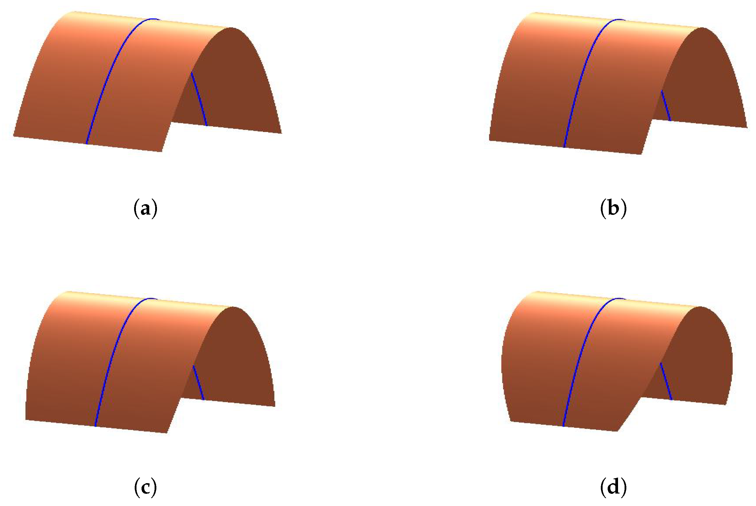
In this section, we use another approach to construct the developable surface. Take the second derivative of Equation (7), which is
x 0 ( t ) x + x 1 ( t ) y + x 2 ( t ) z = x 3 ( t ) .
By Definition 3, three consecutive planes in the plane family { t } intersect a characteristic point. We can obtain this point by solving the following equation system:
x 0 ( t ) x + x 1 ( t ) y + x 2 ( t ) z = x 3 ( t ) , x 0 ( t ) x + x 1 ( t ) y + x 2 ( t ) z = x 3 ( t ) , x 0 ( t ) x + x 1 ( t ) y + x 2 ( t ) z = x 3 ( t ) .
According to Cramer’s Rule, the coordinate of the intersection q ( t ) is given by
x = x 3 ( t ) x 1 ( t ) x 2 ( t ) x 3 ( t ) x 1 ( t ) x 2 ( t ) x 3 ( t ) x 1 ( t ) x 2 ( t ) x 0 ( t ) x 1 ( t ) x 2 ( t ) x 0 ( t ) x 1 ( t ) x 2 ( t ) x 0 ( t ) x 1 ( t ) x 2 ( t ) , y = x 0 ( t ) x 3 ( t ) x 2 ( t ) x 0 ( t ) x 3 ( t ) x 2 ( t ) x 0 ( t ) x 3 ( t ) x 2 ( t ) x 0 ( t ) x 1 ( t ) x 2 ( t ) x 0 ( t ) x 1 ( t ) x 2 ( t ) x 0 ( t ) x 1 ( t ) x 2 ( t ) , z = x 0 ( t ) x 1 ( t ) x 3 ( t ) x 0 ( t ) x 1 ( t ) x 3 ( t ) x 0 ( t ) x 1 ( t ) x 3 ( t ) x 0 ( t ) x 1 ( t ) x 2 ( t ) x 0 ( t ) x 1 ( t ) x 2 ( t ) x 0 ( t ) x 1 ( t ) x 2 ( t ) .
When parameter t changes in [ 0 , 1 ] , q ( t ) can generate a spine curve. We construct the parametric surface as
T ( t , v ) = q ( t ) + v q ( t ) , t [ 0 , 1 ] , v ( , ) ,
which is a tangent developable surface with q ( t ) as its line of regression. Then, we analyze the property of the developable surface ( 12 ) . We take the second derivative of Equation ( 6 ) . When t = 0 and t = 1 , we put it with Equations ( 10 ) and ( 11 ) together:
X ( 0 ; α 1 , α 2 , α 3 ) = Q 0 , X ( t ; α 1 , α 2 , α 3 ) = δ 0 , 2 ( Q 1 Q 0 ) , X ( 0 ; α 1 , α 2 , α 3 ) = δ 0 , 2 δ 0 , 1 ( Q 0 Q 1 ) + δ 1 , 2 δ 0 , 1 ( Q 2 Q 1 ) ,
and
X ( 1 ; α 1 , α 2 , α 3 ) = Q 3 , X ( t ; α 1 , α 2 , α 3 ) = δ 2 , 2 ( Q 1 Q 0 ) , X ( 1 ; α 1 , α 2 , α 3 ) = δ 1 , 2 δ 1 , 1 ( Q 1 Q 2 ) + δ 2 , 2 δ 1 , 1 ( Q 3 Q 2 ) .
Due to Definition 3, the intersection of the control planes Q 0 , Q 1 , Q 2 is the characteristic point which lies on the generator T ( 0 ; α 1 , α 2 , α 3 ) . Similarly, the intersection of the control planes Q 1 , Q 2 , Q 3 is on the generator T ( 1 ; α 1 , α 2 , α 3 ) . The following example shows the effects of the parameters α 1 , α 2 , α 3 for surface T ( t , v ) .
Example 3.
The coordinates of the control planes are
Q 0 = ( 2 3 , 6 , 2 3 , 60 ) , Q 1 = ( 3 3 , 9 , 3 3 , 135 ) , Q 2 = ( 4 3 , 12 , 4 3 , 240 ) , Q 3 = ( 5 3 , 15 , 5 3 , 375 ) .
FromFigure 7,Figure 8andFigure 9, we can see the following influence of parameters on the developable surface:
  • When modifying the value of α 1 and keeping α 2 , α 3 unchanged, the length and position of the generator T ( 0 ; α 1 , α 2 , α 3 ) remain the same. The position of the generator T ( 1 ; α 1 , α 2 , α 3 ) remains unchanged, but the length of it becomes shorter when we increase the value of α 1 .
  • When we only change the value of α 2 , the generator T ( 0 ; α 1 , α 2 , α 3 ) and T ( 1 ; α 1 , α 2 , α 3 ) have no changes in position and length. However, the lengths of the two generators become shorter when increasing the value of α 2 .
  • We just modify the value of α 3 , the position and the length of the generator T ( 1 ; α 1 , α 2 , α 3 ) remain unchanged. The position of the generator T ( 0 ; α 1 , α 2 , α 3 ) also has no change, but the length of it will become shorter when increasing the value of α 3 .

4. 1 × 3 Developable Surface Interpolating Cubic Geodesic C-Bézier Curve with Parameters

Geodesic is an important characteristic curve on surface. In this section, we construct a developable surface through the given C-Bézier curve, and the curve is the geodesic of the surface.
Theorem 1
([26]). A curve (not a line) is a geodesic on the surface T ( t , v ) if and only if, at any point on the curve, the principal normal β ( t ) to the curve is parallel to the normal N ( t , v 0 ) .
Proof. 
Assume C ( t ) is a curve on the surface T ( t , v ) , and P is an arbitrary point on C ( t ) . β ( t ) is the principal normal, N ( t , v 0 ) is the normal vector at point P , θ is the angle between β ( t ) and N ( t , v 0 ) , and k g is the geodesic curvature. According to the definitions of the geodesic curvature and geodesic curve, we have
k g = ± k sin θ = 0 .
Because k 0 , then θ = 0 or θ = π , that is, β ( t ) is parallel to N ( t , v 0 ) . The conclusion is proved. □
Theorem 2.
Given a C-Bézier curve with parameters α 1 , α 2 , α 3 , there must exist a developable surface through it that is the geodesic of the developable surface.
Proof. 
Given a space cubic C-Bézier curve P ( t ; α 1 , α 2 , α 3 ) , we have the corresponding ruled surface
T ( t , v ; α 1 , α 2 , α 3 ) = P ( t ; α 1 , α 2 , α 3 ) + v P 1 ( t ; α 1 , α 2 , α 3 ) , ( t [ 0 , 1 ] , v ( , ) ) .
If P ( t ; α 1 , α 2 , α 3 ) is geodesic, by Theorem 1, we have
T ( t , 0 ; α 1 , α 2 , α 3 ) = P ( t ; α 1 , α 2 , α 3 ) , β ( t , α 1 , α 2 , α 3 ) N ( t , 0 ; α 1 , α 2 , α 3 ) ,
where N ( t , 0 ; α 1 , α 2 , α 3 ) and β ( t ; α 1 , α 2 , α 3 ) are the normal vector and the principal normal vector of the curve. To make the writing simple, we omit the variable and parameters in the following process of this theorem:
N ( t , 0 ; α 1 , α 2 , α 3 ) = T t × T v = ( P + v P 1 ) × P 1 | v = 0 = P × P 1 , β ( t , α 1 , α 2 , α 3 ) = ( P · P ) · P ( P · P ) · P | P | | P × P | .
Because P N and β ( t ; α 1 , α 2 , α 3 ) N ( t , 0 ; α 1 , α 2 , α 3 ) , then the vector P 1 must lie in the plane spanned by P and P × P . We let
P 1 = λ 1 P + λ 2 ( P × P ) .
According to the developable conditions, we have
( P , λ 1 P + λ 2 ( P × P ) , ( λ 1 P + λ 2 ( P × P ) ) ) = 0 ( P , λ 1 P + λ 2 ( P × P ) , λ 1 P + λ 1 P + λ 2 P × P + λ 2 P × P ) = 0 ( P , λ 2 ( P × P ) , λ 1 P + λ 2 P × P + λ 2 P × P ) = 0 λ 2 0 [ ( P × P ) × P ] · ( λ 1 P + λ 2 P × P ) = 0 [ ( P · P ) P ( P · P ) P ] · ( λ 1 P + λ 2 P × P ) = 0 ( | P | 2 | P | 2 | P · P | 2 ) λ 1 = | P | 2 ( P , P , P ) λ 2 .
That is, there must exist a developable surface
T ( t , v ; α 1 , α 2 , α 3 ) = P ( t ; α 1 , α 2 , α 3 ) + v ( λ 1 P ( t ; α 1 , α 2 , α 3 ) + λ 2 ( P ( t ; α 1 , α 2 , α 3 ) × P ( t ; α 1 , α 2 , α 3 ) ) , ( t [ 0 , 1 ] , v ( , ) ) ,
which interpolates the given curve P ( t ) , and P ( t ) is the geodesic of the developable surface, where λ 1 ( t ) a n d λ 2 ( t ) satisfy Equation (13). ☐
In a special case, if we choose λ 2 ( t ) = 1 , then Equation ( 14 ) can be expressed as (we omit the variable and parameters)
T = P + v ( | P | 2 ( P , P , P ) | P | 2 | P | 2 | P · P | 2 P + P × P ) , t [ 0 , 1 ] , v ( , ) .
We will give an example to illustrate that the constructed method is effective.
Example 4.
The control points are P 0 = [ 0 , 0 , 0 ] , P 1 = [ 1 , 0 , 1 ] , P 2 = [ 2 , 0 , 1 ] , P 3 = [ 3 , 0 , 0 ] , and we construct a developable surface interpolating the curve generated by the given control points, and at the same time the curve is the geodesic of the developable surface. We just observe that the parameters have influences on the developable surface fromFigure 10,Figure 11andFigure 12. However, recently, it has been hard to analyze the geometric meaning of parameters from theory. We will consider it further in our future work.

5. Conclusions

In this paper, we define some new basis functions that are the generalization of the C-Bézier basis. These basis functions not only have the similar properties with Bézier basis, but also have the better handling when using them to generate curve and surface. Based on the new basis, we construct developable surface through cubic curves by single parameter plane family and tangent surface of the spine curve, respectively. The main advantage compared to the ordinary C-Bézier curve and surface is that we can design them flexibly by suitably modifying the values of the shape parameters either locally or globally. According to the good property of endpoints interpolating and derivatives, we analyzed the relationship between control planes and the generators of the developable surface at t = 0 and t = 1 , respectively. The examples also show the influence on the developable surfaces when we just change one parameter and keep other parameters unchanged.
Our main point in this paper is the mathematical theory and properties of C-Bézier curve with n parameters. Under these basis functions, the developable surface can be controlled easily. As an extension of classic developable Bézier surfaces, the generalized developable C-Bézier surfaces provide a new class of mathematical theory for the development of CAD/CAM application software. Some interesting results in this area are taken into account, and they will be discussed in our future works. We will develop the application from the following aspects:
  • In the CAD/CAM field, the modeling of some products are often built by blending multiple developable patches together. Therefore, in the future, we will study the conditions of G 1 and G 2 Beta continuity of new C-Bézier developable surfaces and analyze the effects of shape parameters on the composite surface. We will try to apply the composite C-Bézier developable surface with parameters to design the car body, shoes, ship hull, etc. I think it will be a useful complement for CAD/CAM.
  • Moreover, many researchers discussed the trigonometric curve and surface with some parameters; refer to [27,28,29]. We also want to extend our work to trigonometric curve and surface with some parameters, which can be controlled due to the freedom provided by these parameters. They can be efficient models in the fields of CAGD.
  • Yang and Liang [23] presented a new kind of algebraic-trigonometric blended spline curve, called x y B curves. The new curves can represent some conics and transcendental curves. We can extend our work to the C-B-spline curve and surface with n parameters. We will try to construct a spline curve to interpolate given points and to represent some conic curves. Because of more freedom, we may get more smooth and precise curves.

Author Contributions

Formal analysis, C.L.; Funding acquisition, C.Z.; Investigation, C.L.; Methodology, C.L.; Supervision, C.Z.; Writing—original draft, C.L. All authors have read and agreed to the published version of the manuscript.

Funding

This work is partly supported by the National Natural Science Foundation of China (Nos. 11401077, 11671068, 11271060).

Conflicts of Interest

The authors declare no conflict of interest.

References

  1. Aumann, G. Interpolation with developable Bézier patches. Comput. Aided Geom. Des. 1991, 8, 409–420. [Google Scholar] [CrossRef]
  2. Lang, J.; Ro¨schel, O. Developable (1,n)-Bézier surfaces. Comput. Aided Geom. Des. 1992, 9, 291–298. [Google Scholar] [CrossRef]
  3. Chalfant, J.S.; Maekawa, T. Design for manufacturing using B-Spline developable surfaces. J. Ship Prod. 1998, 42, 207–215. [Google Scholar]
  4. Pottmann, H.; Farin, G. Developable rational Bézier and B-spline surfaces. Comput. Aided Geom. Des. 1995, 12, 513–531. [Google Scholar] [CrossRef]
  5. Chu, C.H.; Séquin, C.H. Developable Bézier patches: Properties and design. Comput. Aided Des. 2002, 34, 511–527. [Google Scholar] [CrossRef]
  6. Bodduluri, R.M.C.; Ravani, B. Geometric design and fabrication of developable Bézier and B-spline surfaces. ASME Trans. J. Mech. Des. 1994, 116, 1024–1048. [Google Scholar] [CrossRef]
  7. Bodduluri, R.M.C.; Ravani, B. Design of developable surfaces using duality between plane and point geometies. Comput. Aided Des. 1993, 25, 621–632. [Google Scholar] [CrossRef]
  8. Zhao, H.Y.; Wang, G.J. A new method for designing a developable surface utilizing the surface pencil through a given curve. Prog. Nat. Sci. 2008, 18, 105–110. [Google Scholar] [CrossRef]
  9. Li, C.Y.; Wang, R.H.; Zhu, C.G. An approach for designing a developable surface through a given line of curvature. Comput. Aided Des. 2013, 45, 621–627. [Google Scholar] [CrossRef]
  10. Farin, G. Rational curves and surfaces. In Mathematical Methods in Computer Aided Geometric Design; Lyche, T., Schumaker, I., Eds.; Academic Press: Boston, MA, USA, 1989. [Google Scholar]
  11. Piegl, I. On NURBS: A survey. IEEE Comput. Graph. Appl. 1991, 11, 55–71. [Google Scholar] [CrossRef]
  12. Farin, G. From conics to NURBS: A tutorial and survey. IEEE Comput. Graph. Appl. 1992, 1, 78–86. [Google Scholar] [CrossRef]
  13. Zhang, J.W. C-curves: An extension of cubic curves. Comput. Aided Geom. Des. 1996, 13, 199–217. [Google Scholar] [CrossRef]
  14. Zhang, J.W. Two different forms of C-B splines. Comput. Aided Geom. Des. 1997, 14, 31–41. [Google Scholar] [CrossRef]
  15. Zhang, J.W. C-Bézier Curves and Surfaces. Graph. Models Ima Process. 1999, 61, 2–15. [Google Scholar] [CrossRef]
  16. Han, X.A.; Ma, Y.C.; Huang, X.L. A novel generalization of Bezier curve and surface. J. Comput. Appl. Math. 2008, 217, 180–193. [Google Scholar] [CrossRef] [Green Version]
  17. Zhu, Y.P.; Han, X.L. New cubic rational basis with tension shape parameters. Appl. Math. J. Chin. Univ. 2015, 30, 273–298. [Google Scholar] [CrossRef]
  18. Zhu, Y.P.; Han, X.L.; Liu, S.J. Curve construction based on four αβ-Bernstein-like basis functions. J. Comput. Appl. Math. 2015, 273, 160–181. [Google Scholar] [CrossRef]
  19. Zhou, M.; Yang, J.Q.; Zheng, H.C.; Song, W.J. Design and shape adjustment of developable surfaces. Appl. Math. Model. 2013, 37, 3789–3801. [Google Scholar] [CrossRef]
  20. Hu, G.; Cao, H.X.; Qin, X.Q.; Wang, X. Geometric design and continuity conditions of developable λ-Bézier surfaces. Adv. Eng. Softw. 2017, 114, 235–245. [Google Scholar] [CrossRef]
  21. Hu, G.; Wu, J.L.; Qin, X.Q. A new approach in designing of local controlled developable H-Bézier surfaces. Adv. Eng. Softw. 2018, 121, 26–38. [Google Scholar] [CrossRef]
  22. Wang, C.W. Cubic trigonometric polynomial spline curves with shape parameter. J. Beijing Inst. Cloth. Technol. (Nat. Sci. Ed.) 2008, 28, 50–55. [Google Scholar]
  23. Yang, L.L.; Liang, J.F. A class of algebraic-trigonometric blended splines. J. Comput. Appl. Math. 2011, 235, 1713–1729. [Google Scholar]
  24. Chen, Q.Y.; Wang, G.Z. A class of Bézier-like curves. Comput. Aided Geom. Des. 2003, 20, 29–39. [Google Scholar] [CrossRef]
  25. Shang, Y.L. Consensus formation of two-level opinion dynamics. Acta Math. Sci. 2014, 34B, 1029–1040. [Google Scholar] [CrossRef]
  26. Carmo, M.D. Differential Geometry of Curves and Surfaces; Prentice Hall: Englewood Cliffs, NJ, USA, 1976. [Google Scholar]
  27. Sharma, R. Quartic Trigonometric Bézier Curves and Surfaces with Shape Parameter. Int. J. Innov. Res. Comput. Commun. Eng. 2016, 3297, 7712–7717. [Google Scholar]
  28. Bashir, U.; Abbas, M.; Awang, M.; Ali, J.M. A class of quasi-quintic trigonometric Bézier curve with two shape parameters. Sci. Asia 2013, 39S, 11–15. [Google Scholar] [CrossRef] [Green Version]
  29. Misro, M.Y.; Ramli, A.; Ali, J.M. Quintic trigonometric Bézier curve with two shape parameters. Sains Malays. 2017, 46, 825–831. [Google Scholar]
Figure 1. Quadratic basis functions. (a) α 1 = π 8 , α 2 = π 8 ; (b) α 1 = π 8 , α 2 = 7 π 8 ; (c) α 1 = 7 π 8 , α 2 = π 8 ; and (d) α 1 = 7 π 8 , α 2 = 7 π 8 .
Mathematics 08 00402 g001
Figure 2. Cubic basis functions. (a) α 1 = π 8 , α 2 = π 8 , α 3 = π 8 ; (b) α 1 = 13 π 8 , α 2 = 13 π 8 , α 3 = 13 π 8 ; (c) α 1 = π 8 , α 2 = 13 π 8 , α 3 = π 8 ; (d) α 1 = 13 π 8 , α 2 = π 8 , α 3 = 13 π 8 ; (e) α 1 = π 8 , α 2 = π 8 , α 3 = 13 π 8 ; (f) α 1 = 13 π 8 , α 2 = π 8 , α 3 = π 8 .
Mathematics 08 00402 g002
Figure 3. Cubic C-Bézier curves with different parameters. (a) α 1 = [ π 8 , π 8 , π 8 , 13 π 8 ] ; α 2 = [ 13 π 8 , π 8 , π 8 , π 8 ] ; α 3 = [ π 8 , 13 π 8 , π 8 , π 8 ] ; ( b ) α 1 = [ π 8 , π 8 , π 8 , 13 π 8 ] ; α 2 = [ 13 π 8 , π 8 , π 8 , π 8 ] ; α 3 = [ π 8 , 13 π 8 , π 8 , π 8 ] .
Mathematics 08 00402 g003
Figure 4. The effects of parameter α 1 on the 1 × 3 developable surface. (a) α 1 = π 4 , α 2 = π 4 , α 3 = π 4 ; (b) α 1 = π 2 , α 2 = π 4 , α 3 = π 4 ; (c) α 1 = 3 π 4 , α 2 = π 4 , α 3 = π 4 ; and (d) α 1 = π , α 2 = π 4 , α 3 = π 4 .
Mathematics 08 00402 g004
Figure 5. The effects of parameter α 2 on the 1 × 3 developable surface. (a) α 1 = π 4 , α 2 = π 4 , α 3 = π 4 ; (b) α 1 = π 4 , α 2 = π 2 , α 3 = π 4 ; (c) α 1 = π 4 , α 2 = 3 π 4 , α 3 = π 4 ; and (d) α 1 = π 4 , α 2 = 5 π 4 , α 3 = π 4 .
Mathematics 08 00402 g005
Figure 6. The effects of parameter α 3 on the 1 × 3 developable surface. (a) α 1 = π 4 , α 2 = π 4 , α 3 = π 4 ; (b) α 1 = π 4 , α 2 = π 4 , α 3 = π 2 ; (c) α 1 = π 4 , α 2 = π 4 , α 3 = 3 π 4 ; and (d) α 1 = π 4 , α 2 = π 4 , α 3 = π .
Mathematics 08 00402 g006
Figure 7. The effects of parameter α 1 on the tangent developable surface. (a) α 1 = π 4 , α 2 = π 4 , α 3 = π 4 ; (b) α 1 = π 2 , α 2 = π 4 , α 3 = π 4 ; (c) α 1 = 3 π 4 , α 2 = π 4 , α 3 = π 4 ; and (d) α 1 = π , α 2 = π 4 , α 3 = π 4 .
Mathematics 08 00402 g007
Figure 8. The effects of parameter α 2 on the tangent developable surface. (a) α 1 = π 4 , α 2 = π 4 , α 3 = π 4 ; (b) α 1 = π 4 , α 2 = π 2 , α 3 = π 4 ; (c) α 1 = π 4 , α 2 = 3 π 4 , α 3 = π 4 ; and (d) α 1 = π 4 , α 2 = 5 π 4 , α 3 = π 4 .
Mathematics 08 00402 g008
Figure 9. The effects of parameter α 3 on the tangent developable surface. (a) α 1 = π 4 , α 2 = π 4 , α 3 = π 4 ; (b) α 1 = π 4 , α 2 = π 4 , α 3 = π 2 ; (c) α 1 = π 4 , α 2 = π 4 , α 3 = 3 π 4 ; and (d) α 1 = π 4 , α 2 = π 4 , α 3 = π .
Mathematics 08 00402 g009
Figure 10. The effects of parameter α 1 on the developable surface through geodesic. (a) α 1 = π 4 , α 2 = π 4 , α 3 = π 4 ; (b) α 1 = π 2 , α 2 = π 4 , α 3 = π 4 ; (c) α 1 = 3 π 4 , α 2 = π 4 , α 3 = π 4 ; and (d) α 1 = π , α 2 = 5 π 4 , α 3 = π 4 .
Mathematics 08 00402 g010
Figure 11. The effects of parameter α 2 on the developable surface through geodesic. (a) α 1 = π 4 , α 2 = π 4 , α 3 = π 4 ; (b) α 1 = π 4 , α 2 = π 2 , α 3 = π 4 ; (c) α 1 = π 4 , α 2 = 3 π 4 , α 3 = π 4 ; and (d) α 1 = π 4 , α 2 = 5 π 4 , α 3 = π 4 .
Mathematics 08 00402 g011
Figure 12. The effects of parameter α 2 on the developable surface through geodesic. (a) α 1 = π 4 , α 2 = π 4 , α 3 = π 4 ; (b) α 1 = π 4 , α 2 = π 4 , α 3 = π 2 ; (c) α 1 = π 4 , α 2 = π 4 , α 3 = 3 π 4 ; and (d) α 1 = π 4 , α 2 = π 4 , α 3 = π .
Mathematics 08 00402 g012

