Review

Finite Difference Method for the Multi-Asset Black–Scholes Equations

1
Department of Mathematics, Korea University, Seoul 02841, Korea
2
Department of Mathematics, Kangwon National University, Gangwon-do 24341, Korea
*
Author to whom correspondence should be addressed.
Mathematics 2020, 8(3), 391; https://doi.org/10.3390/math8030391
Submission received: 13 January 2020 / Revised: 28 February 2020 / Accepted: 6 March 2020 / Published: 10 March 2020
(This article belongs to the Special Issue Open Source Codes for Numerical Analysis)

Abstract

:
In this paper, we briefly review the finite difference method (FDM) for the Black–Scholes (BS) equations for pricing derivative securities and provide the MATLAB codes in the Appendix for the one-, two-, and three-dimensional numerical implementation. The BS equation is discretized non-uniformly in space and implicitly in time. The two- and three-dimensional equations are solved using the operator splitting method. In the numerical tests, we show characteristic examples for option pricing. The computational results are in good agreement with the closed-form solutions to the BS equations.

1. Introduction

The well-known Black–Scholes (BS) partial differential equation (PDE) [1,2] is an accurate and efficient mathematical model for option pricing. The pioneers F. Black, M. Scholes, and R. Merton made a great breakthrough in the option pricing; and M. Scholes and R. Merton received in 1997 the Nobel Prize for their discovery of the BS equation. A European call option is a contract that gives the owner the right to buy an asset with a strike price K at an expiration date T. Let u ( s 1 , s 2 , , s n , t ) be the value of the option, where s i is the underlying i-th asset value. We consider the following generalized n-asset BS equation [3,4]:
u ( s , t ) t + 1 2 i , j = 1 n σ i σ j ρ i j s i s j 2 u ( s , t ) s i s j + r i = 1 n s i u ( s , t ) s i = r u ( s , t ) ,
for ( s , t ) = ( s 1 , s 2 , , s n , t ) R + n × [ 0 , T ) . The final condition is
u ( s , T ) = u T ( s ) .
Here, r is an interest rate, σ i is a constant volatility of the i-th asset, and ρ i j is the correlation coefficient between i-th and j-th underling assets.
The finite difference method (FDM) has been used for numerically solving the BS equations. In FDM, a PDE is replaced by discrete equations by using the Taylor series approximations to the partial derivatives. Then, we solve the resulting discrete equations by using various numerical methods [5]. Jeong et al. [6] developed the FDM without the far-field boundary condition. Hout and Valkov [7] obtained the European two-asset options by the FDM based numerical method considering non-uniform grids. For high-order option pricing schemes, there are the Crandall–Douglas method [8], the Crank–Nicolson method [9,10], and second-order in time and fourth-order in space method [11]. In [12], Zhao and Tian investigated FDMs for solving the fractional BS equation, and studied the stability and convergence of the proposed first- and second-order implicit numerical schemes. Chen and Wang [13] presented a second-order Crank–Nicolson alternating direction implicit (ADI) scheme for solving a 2D spatial fractional BS equation. Sawangtong et al. [14] proposed the BS equation with two assets based on the Liouville–Caputo fractional derivative. In [15], Zhan et al. developed numerical methods for the time fractional BS equation. Hu and Gan [16] developed a fourth-order scheme for the BS PDE. In [17], Hendricks et al. combined high-order FDM with an ADI scheme for the BS equation in a sparse grid setting. In [18], Rao proposed an FDM for a generalized BS equation (non-constant interest rate and volatility) and proved that the scheme is second-order accurate spatially and temporally. In [19], Ullah presented numerical solution of three dimensional Heston–Hull–White (HHW) model using a high order FDM. The HHW model applies to pricing options arising from the probabilistic nature of asset prices, volatility, and risk-free interest rates. In [9], Ankudinova and Ehrhardt presented numerical methods for the nonlinear BS equation [20].
The main contribution of this paper is to present the detailed FDM for the BS equations for pricing derivative securities and provide the MATLAB codes for the one-, two-, and three-dimensional numerical implementation so that the beginners can use the provided codes for their research projects without wasting time for debugging the implementation [21].
The outline of this paper is as follows. The numerical solutions of the one-, two-, and three-dimensional BS equation are briefly described in Section 2. In 
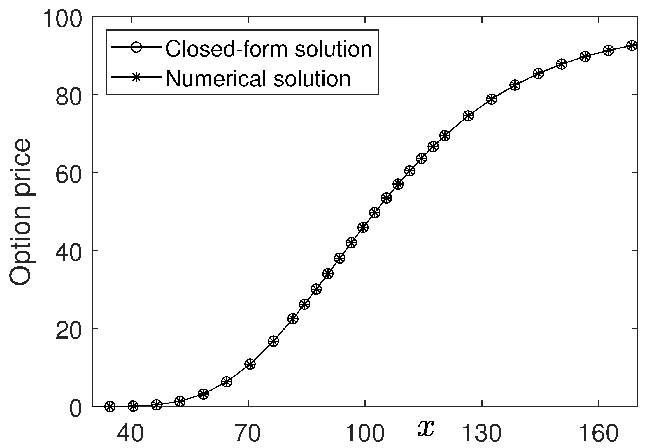
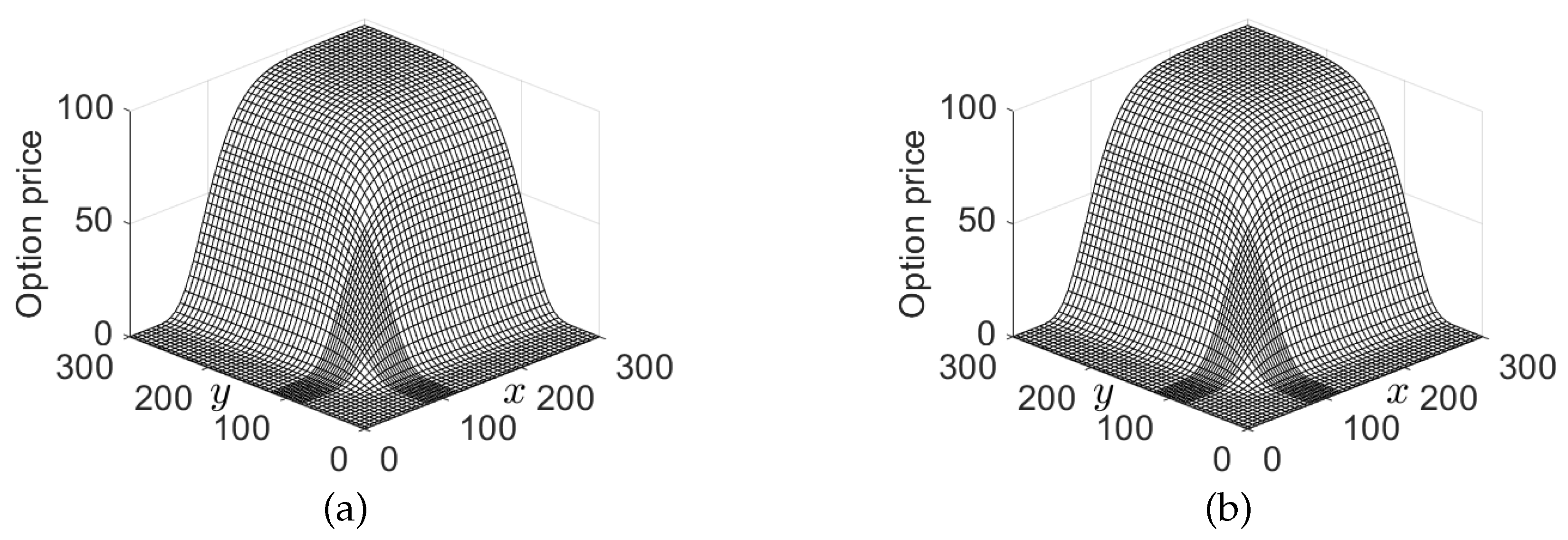
Section 3, we present the numerical results of cash-or-nothing options in order to show the accuracy and efficiency. We finalize the paper with the conclusion in Section 4. In the Appendix A, we provide the MATLAB codes for the numerical implementation for one-, two-, and three-dimensions.

2. Numerical Solutions

By changing the variable with τ = T t , Equation (1) becomes
u ( s , τ ) τ = 1 2 i , j = 1 n σ i σ j ρ i j s i s j 2 u ( s , τ ) s i s j + r i = 1 n s i u ( s , τ ) s i r u ( s , τ ) .
The initial condition is u ( s , 0 ) = u T ( s ) . Let us consider the numerical solution algorithm for the three-dimensional BS equation. The algorithms for the one- and two-dimensional BS equations are similarly defined. Let x = s 1 , y = s 2 , and z = s 3 . Let L B S be the following operator:
L B S u = 1 2 σ x 2 x 2 2 u x 2 + 1 2 σ y 2 y 2 2 u y 2 + 1 2 σ z 2 z 2 2 u z 2 + ρ x y σ x σ y x y 2 u x y + ρ y z σ y σ z y z 2 u y z + ρ z x σ z σ x z x 2 u z x + r x u x + r y u y + r z u z r u .
Then, the BS equation can be written as
u τ = L B S u for ( x , y , z , τ ) Ω × ( 0 , T ] , u ( x , y , z , 0 ) = u T ( x , y , z ) ,
where τ = T t . We truncate the original infinite domain into a finite domain Ω = ( 0 , L ) × ( 0 , M ) × ( 0 , N ) . We discretize Ω with a non-uniform space step h i x = x i + 1 x i , h j y = y j + 1 y j , h k z = z k + 1 z k for i = 0 , , N x 1 , j = 0 , , N y 1 , and k = 0 , , N z 1 . Here, x 0 = y 0 = z 0 = 0 , x N x = L , y N y = M , and z N z = N . A time step is Δ τ = T / N τ . 
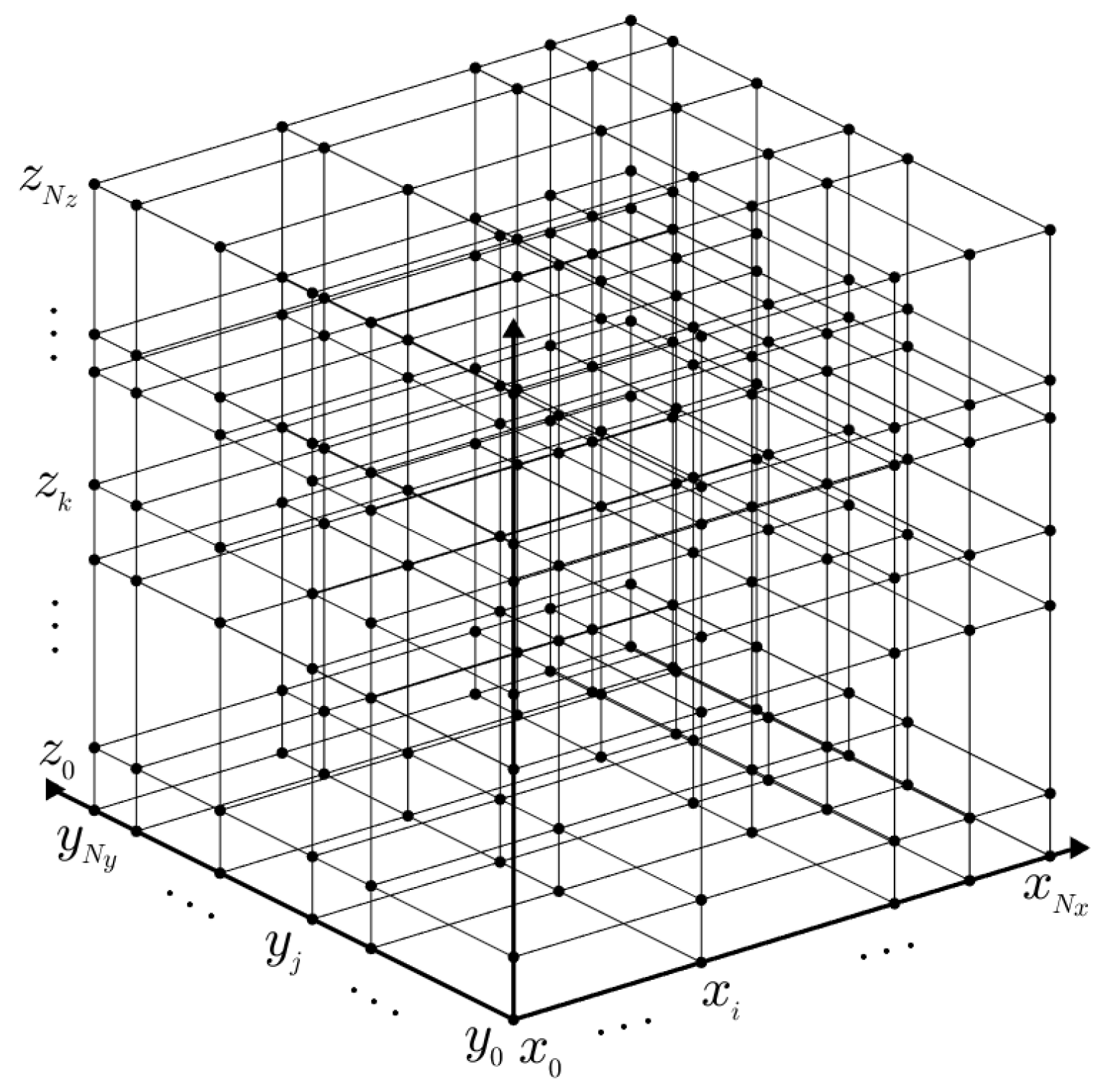
Figure 1 is an example of 3D non-uniform grid.
Let u i j K n = u x i , y j , z k , n Δ τ , where i = 0 , , N x , j = 0 , , N y , k = 0 , , N z , and n = 0 , , N τ . We use the zero Dirichlet boundary condition: u ( 0 , y , z , τ ) = u ( x , 0 , z , τ ) = u ( x , y , 0 , τ ) = 0 for 0 x L , 0 y M , 0 z N , 0 τ T , i.e., u 0 j k n = 0 for j = 0 , , N y , k = 0 , , N z , u i 0 k n = 0 for i = 0 , , N x , k = 0 , , N z , and u i j 0 n = 0 for i = 0 , , N x , j = 0 , , N y ; and the homogeneous Neumann boundary condition: u x ( L , y , z , τ ) = u y ( x , M , z , τ ) = u z ( x , y , N , τ ) = 0   for   0 x L , 0 y M , 0 z N , 0 τ T , that is, u N x + 1 , j k n = u N x , j k n for j = 0 , , N y , k = 0 , , N z , u i , N y + 1 , k n = u i , N y , k n for i = 0 , , N x , k = 0 , , N z , and u i j , N z + 1 n = u i j , N z n for i = 0 , , N x , j = 0 , , N y .
Now, we apply the operator splitting (OS) method [22,23] to solve Equation (5). We consider the following three discrete equations:
u i j k n + 1 3 u i j k n Δ τ = L B S x u i j k n + 1 3 ,
u i j k n + 2 3 u i j k n + 1 3 Δ τ = L B S y u i j k n + 2 3 ,
u i j k n + 1 u i j k n + 2 3 Δ τ = L B S z u i j k n + 1 ,
for 1 i N x , 1 j N y , and 1 k N z . Here, the discrete difference operators L B S x , L B S y , and L B S z are defined by
L B S x u i j k n + 1 3 = σ x x i 2 2 D x x u i j k n + 1 3 + r x i D x u i j k n + 1 3 + 1 3 σ x σ y ρ x y x i y j D x y u i j k n + 1 3 σ y σ z ρ y z y j z k D y z u i j k n + 1 3 σ z σ x ρ z x z k x i D z x u i j k n 1 3 r u i j k n + 1 3 ,
L B S y u i j k n + 2 3 = σ y y j 2 2 D y y u i j k n + 2 3 + r y j D y u i j k n + 2 3 + 1 3 σ x σ y ρ x y x i y j D x y u i j k n + 1 3 + 1 3 σ y σ z ρ y z y j z k D y z u i j k n + 1 3 + 1 3 σ z σ x ρ z x z k x i D z x u i j k n + 1 3 1 3 r u i j k n + 2 3 ,
L B S z u i j k n + 1 = σ z z k 2 2 D z z u i j k n + 1 + r z k D z u i j k n + 1 + 1 3 σ x σ y ρ x y x i y j D x y u i j k n + 2 3 + 1 3 σ y σ z ρ y z y j z k D y z u i j k n + 2 3 + 1 3 σ z σ x ρ z x z k x i D z x u i j k n + 2 3 1 3 r u i j k n + 1 ,
where the first and second derivatives are defined in [24] as
D x u i j k = h i x h i 1 x ( h i 1 x + h i x ) u i 1 , j k + h i x h i 1 x h i 1 x h i x u i j k + h i 1 x h i x ( h i 1 x + h i x ) u i + 1 , j k ,
D y u i j k = h j y h j 1 y ( h j 1 y + h j y ) u i , j 1 , k + h j y h j 1 y h j 1 y h j y u i j k + h j 1 y h j y ( h j 1 y + h j y ) u i , j + 1 , k ,
D z u i j k = h k z h k 1 z ( h k 1 z + h k z ) u i j , k 1 + h k z h k 1 z h k 1 z h k z u i j k + h k 1 z h k z ( h k 1 z + h k z ) u i j , k + 1 ,
D x x u i j k = 2 h i 1 x ( h i 1 x + h i x ) u i 1 , j k 2 h i 1 x h i x u i j k + 2 h i x ( h i 1 x + h i x ) u i + 1 , j k ,
D y y u i j k = 2 h j 1 y ( h j 1 y + h j y ) u i , j 1 , k 2 h j 1 y h j y u i j k + 2 h j y ( h j 1 y + h j y ) u i , j + 1 , k ,
D z z u i j k = 2 h k 1 z ( h k 1 z + h k z ) u i j , k 1 2 h k 1 z h k z u i j k + 2 h k z ( h k 1 z + h k z ) u i j , k + 1 ,
D x y u i j k = u i + 1 , j + 1 , k u i 1 , j + 1 , k u i + 1 , j 1 , k + u i 1 , j 1 , k h i x h j y + h i 1 x h j y + h i x h j 1 y + h i 1 x h j 1 y ,
D y z u i j k = u i , j + 1 , k + 1 u i , j 1 , k + 1 u i , j + 1 , k 1 + u i , j 1 , k 1 h j y h k z + h j 1 y h k z + h j y h k 1 z + h j 1 y h k 1 z ,
D z x u i j k = u i + 1 , j , k + 1 u i + 1 , j , k 1 u i 1 , j , k + 1 + u i 1 , j , k 1 h k z h i x + h k 1 z h i x + h k z h i 1 x + h k 1 z h i 1 x .
Now, we describe the numerical algorithm for Equations (6)–(8). Given u i j k n , Equation (6) is rewritten as follows:
α i u i 1 , j k n + 1 3 + β i u i j k n + 1 3 + γ i u i + 1 , j k n + 1 3 = f i j k ,
where
α i = ( σ x x i ) 2 h i 1 x ( h i 1 x + h i x ) + r x i h i x h i 1 x ( h i 1 x + h i x ) ,
β i = 1 Δ τ + ( σ x x i ) 2 h i 1 x h i x r x i h i x h i 1 x h i 1 x h i x + r 3 , γ i = ( σ x x i ) 2 h i x ( h i 1 x + h i x ) r x i h i 1 x h i x ( h i 1 x + h i x ) ,
f i j k n = 1 3 σ x σ y ρ x y x i y j D x y u i j k n + 1 3 σ y σ z ρ y z y j z k D y z u i j k n + 1 3 σ x σ z ρ z x x i z k D z x u i j k n 1 Δ τ u i j k n .
For fixed indices j and k; and f 1 : N x , j k n = [ f 1 j k n f 2 j k n f N x , j k n ] T , the solution vector u 1 : N x , j k n + 1 3 = [ u 1 j k n + 1 3 u 2 j k n + 1 3 u N x , j k n + 1 3 ] T can be found by solving the tridiagonal system
A x u 1 : N x , j k n + 1 3 = f 1 : N x , j k n ,
where A x is a matrix obtained from Equation (21) with the zero Dirichlet (i.e., u 0 j k n + 1 3 = 0 at x = 0 ) and the one-sided difference for the homogeneous Neumann (i.e., u N x + 1 , j k n + 1 3 = u N x , j k n + 1 3 at x = L ) boundary conditions, that is,
A x = β 1 γ 1 0 0 0 α 2 β 2 γ 2 0 0 0 α 3 β 3 0 0 0 0 0 β N x 1 γ N x 1 0 0 0 α N x β N x + γ N x .
To generate a tridiagonal matrix A x of Equation (26) in MATLAB, see Listing 1, we use the diag ( V , n ) function which returns a square matrix with the elements of input vector V on the n-th diagonal. For example, option n = 0 , n = 1 , and n = 1 place the elements of input vector V on the main-, first super-, and first sub-diagonal, respectively.
Listing 1: Generating a tridiagonal matrix A x .
Mathematics 08 00391 i001
Similarly, Equation (7) is rewritten as matrix form:
α j u i , j 1 , k n + 2 3 + β j u i j k n + 2 3 + γ j u i , j + 1 , k n + 2 3 = f i j k n + 1 3 ,
where
α j = ( σ y y j ) 2 h j 1 y ( h j 1 y + h j y ) + r y j h j y h j 1 y ( h j 1 y + h j y ) ,
β j = 1 Δ τ + ( σ y y j ) 2 h j 1 y h j y r y j h j y h j 1 y h j 1 y h j y + r 3 , γ j = ( σ y y j ) 2 h j y ( h j 1 y + h j y ) r y j h j 1 y h j y ( h j 1 y + h j y ) ,
f i j k n + 1 3 = 1 3 σ x σ y ρ x y x i y j D x y u i j k n + 1 3 + 1 3 σ y σ z ρ y z y j z k D y z u i j k n + 1 3 + 1 3 σ z σ x ρ z x z k x i D z x u i j k n + 1 3 1 Δ τ u i j k n + 1 3 .
For fixed indices i and k; and f i , 1 : N y , k n + 1 3 = [ f i 1 k n + 1 3 f i 2 k n + 1 3 f i , N y , k n + 1 3 ] T , the solution vector u i , 1 : N y , k n + 2 3 = [ u i 1 k n + 2 3 u i 2 k n + 2 3 u i , N y , k n + 2 3 ] T can be obtained by
A y u i , 1 : N y , k n + 2 3 = f i , 1 : N y , k n + 1 3 ,
where A y is a matrix obtained from Equation (27) with the zero Dirichlet (i.e., u i 0 k n + 2 3 = 0 at y = 0 ) and the one-sided difference for the homogeneous Neumann (i.e., u i , N y + 1 , k n + 2 3 = u i , N y , k n + 2 3 at y = M ) boundary conditions, that is,
A y = β 1 γ 1 0 0 0 α 2 β 2 γ 2 0 0 0 α 3 β 3 0 0 0 0 0 β N y 1 γ N y 1 0 0 0 α N y β N y + γ N y .
The process of generating a tridiagonal matrix A y is similar to that of generating A x and the code is as follows Listing 2.
Listing 2: Generating a tridiagonal matrix A y .
Mathematics 08 00391 i002
Finally, Equation (8) is rewritten as matrix form:
α k u i j , k 1 n + 1 + β k u i j k n + 1 + γ k u i j , k + 1 n + 1 = f i j k n + 2 3 ,
where
α k = ( σ z z k ) 2 h k 1 z ( h k 1 z + h k z ) + r z k h k z h k 1 z ( h k 1 z + h k z ) ,
β k = 1 Δ τ + ( σ z z k ) 2 h k 1 z h k z r z k h k z h k 1 z h k 1 z h k z + r 3 , γ k = ( σ z z k ) 2 h k z ( h k 1 z + h k z ) r z k h k 1 z h k z ( h k 1 z + h k z ) ,
f i j k n + 2 3 = 1 3 σ x σ y ρ x y x i y j D x y u i j k n + 2 3 + 1 3 σ y σ z ρ y z y j z k D y z u i j k n + 2 3 + 1 3 σ z σ x ρ z x z k x i D z x u i j k n + 2 3 1 Δ τ u i j k n + 2 3 .
For fixed indices i and j; and f i j , 1 : N z n + 2 3 = [ f i j 1 n + 2 3 f i j 2 n + 2 3 f i j , N z n + 2 3 ] T , the solution vector u i j , 1 : N z n + 1 = [ u i j 1 n + 1 u i j 2 n + 1 u i j , N z n + 1 ] T can be found by solving the tridiagonal system
A z u i j , 1 : N z n + 1 = f i j , 1 : N z n + 2 3 ,
where A z is a matrix obtained from Equation (33) with the zero Dirichlet (i.e., u i j 0 n + 1 = 0 at z = 0 ) and the one-sided difference for the homogeneous Neumann (i.e., u i j , N z + 1 n + 1 = u i j , N z n + 1 at z = N ) boundary conditions, that is,
A z = β 1 γ 1 0 0 0 α 2 β 2 γ 2 0 0 0 α 3 β 3 0 0 0 0 0 β N z 1 γ N z 1 0 0 0 α N z β N z + γ N z .
The code for generating a tridiagonal matrix A z is as follows, Listing 3.
Listing 3: Generating a tridiagonal matrix A z .
Mathematics 08 00391 i003
Then, Equations (6)–(8) are implemented with the following Algorithm 1.
Algorithm 1 Implicit scheme and OSM for three-dimensional Black–Scholes (BS) equation.
  • Require: Previous data u n .
  •   procedure Find the solution u n + 1 3 for Equation (6)
  •     for j = 1 ; j N y ; j + + do
  •         for k = 1 ; k N z ; k + + do
  •            for i = 1 ; i N x ; i + + do
  •                Generate A x and set f i j k n by using Equations (22)–(24)
  •            end for
  •            Solve A x u 1 : N x , j k n + 1 3 = f 1 : N x , j k n
  •         end for
  •     end for
  •   end procedure
  •   procedure Find the solution u n + 2 3 for Equation (7)
  •     for k = 1 ; k N z ; k + + do
  •         for i = 1 ; i N x ; i + + do
  •            for j = 1 ; j N y ; j + + do
  •                Generate A y and set f i j k n + 1 3 by using Equations (28)–(30)
  •            end for
  •            Solve A y u i , 1 : N y , k n + 2 3 = f i , 1 : N y , k n + 1 3
  •         end for
  •     end for
  •   end procedure
  •   procedure Find the solution u n + 1 for Equation (8)
  •     for j = 1 ; j N y ; j + + do
  •         for i = 1 ; i N x ; i + + do
  •            for k = 1 ; k N z ; k + + do
  •                Generate A z and set f i j k n + 2 3 by using Equations (34)–(36)
  •            end for
  •            Solve A z u i j , 1 : N z n + 1 = f i j , 1 : N z n + 2 3
  •         end for
  •     end for
  •   end procedure
To solve the tridiagonal systems found in Equations (25), (31), and (37), we used the backslash operator in MATLAB. Also, interp3() function, which returns interpolated value from a function of three variables at the query points, is used to determine the value at specific query point using the calculated u. The code for Algorithm 1 is as follows, Listing 4:
Listing 4: Code for Algorithm 1.
Mathematics 08 00391 i004

3. Numerical Experiments

We consider one-, two-, and three-asset cash-or-nothing options as test problems. The codes of the payoff function and the closed-form formula are provided below. Unless otherwise specified, we use the following parameters in numerical tests: maturity time T = 1 , time step Δ τ = 0.5 / 365 , risk-free interest rate r = 0.03 , and cash c = 100 . We conduct numerical tests on three non-uniform grids:
Ω 1 = [ 0 , 1.5 , 5.5 , 9.5 , , 77.5 , 80.5 , 83.5 , , 122.5 , 126.5 , 130.5 , 298.5 , 300 ] , Ω 2 = [ 0 , 1 , 4 , 7 , , 79 , 81 , 83 , , 121 , 124 , 127 , , 298 , 300 ] , Ω 3 = [ 0 , 0.5 , 2.5 , 4.5 , , 80.5 , 81.5 , 82.5 , , 120.5 , 122.5 , 124.5 , , 298.5 , 300 ] .
Here, error is defined by the discrete L 2 -norm of relative error between the numerical and the closed-form solutions:
e L 2 = 1 i j k u i j k N τ u ( x i , y j , z k , T ) u ( x i , y j , z k , T ) 2 , for ( x i , y j , z k ) ( 80 , 120 ) × ( 80 , 120 ) × ( 80 , 120 ) ,
where , u i j k N τ and u ( x i , y j , z k , T ) are the number of grid points within the interval ( 80 , 120 ) × ( 80 , 120 ) × ( 80 , 120 ) , the numerical and the closed-form solutions of the cash-or-nothing option, respectively. Here, accuracy is important at the interesting region ( 80 , 120 ) × ( 80 , 120 ) × ( 80 , 120 ) because the payoff of cash-or-nothing is non-smooth and a large volume of trades take place on the neighborhood of the strike K. One- and two-dimensional errors are defined similarly.

3.1. One-Asset Option Test

For the pricing of the one-asset cash-or-nothing option, we use strike price K = 100 , volatility of underlying asset σ = 0.3 , and computational domain Ω = [ 0 , 300 ] . The payoff function of cash-or-nothing option is
u T ( x ) = c , if x K , 0 , otherwise .
The following is the code for the payoff function of the one-asset cash-or-nothing option, see Listing 5:
Listing 5: Pay off of the one-asset cash-or-nothing option.
Mathematics 08 00391 i005
The closed-form formula for the cash-or-nothing option is as follows [25]:
u ( x , τ ) = c e r τ N ( d ) , d = ln ( x K ) + ( r σ 2 2 ) σ τ ,
where the cumulative normal distribution N ( d ) = ( 1 / 2 π ) d e 0.5 ξ 2 d ξ .
The code of the closed-form formula for the cash-or-nothing option is as follows, Listing 6:
Listing 6: Closed-form solution for the one-asset cash-or-nothing option.
Mathematics 08 00391 i006
Here, normcdf(d) function returns the cumulative normal distribution and is evaluated at the value d.
Figure 2 shows the closed-form solution and numerical solution on the grid Ω 3 .
Table 1 lists the numerical solutions of cash-or-nothing option at underlying asset x = 100 and its corresponding error e L 2 with grid Ω i for i = 1 , 2 , 3 .

3.2. Two-Asset Option Test

For pricing two-asset option, we use strike prices K 1 = 100 , K 2 = 100 , volatilities of underlying assets σ x = 0.3 , σ y = 0.3 , the correlation coefficient between two underling assets ρ = 0.5 , and computational domain Ω = [ 0 , 300 ] × [ 0 , 300 ] . The payoff function of cash-or-nothing option with two assets is
u T ( x , y ) = c , if x K 1 , y K 2 , 0 , otherwise .
The code of the payoff function for two-asset cash-or-nothing option is as follows, Listing 7:
Listing 7: Pay off of the two-asset cash-or-nothing option.
Mathematics 08 00391 i007
The closed-form formula for the cash-or-nothing option [25] is
u ( x , y , τ ) = c e r τ B ( d x , d y ; ρ ) , d x = ln x K 1 + r 0.5 σ x 2 τ σ x τ , d y = ln y K 2 + r 0.5 σ y 2 τ σ y τ ,
where the bivariate cumulative normal distribution function B ( α , β ; ρ ) [26] is
B ( d x , d y ; ρ ) = 1 2 π 1 ρ 2 d x d y e ξ 1 2 2 ρ ξ 1 ξ 2 + ξ 2 2 2 1 ρ 2 d ξ 2 d ξ 1 .
The code of the closed-form formula for the two-asset cash-or-nothing option is as follows, Listing 8:
Listing 8: Closed-form solution for the two-asset cash-or-nothing option.
Mathematics 08 00391 i008
In the code, the mvncdf( X , μ , σ ) function returns the multivariate cumulative normal distribution and is evaluated at each row of X. For more information, see the document in MATLAB and [26].
Figure 3a,b show the closed-form and numerical solutions with grid Ω 3 × Ω 3 , respectively.
Table 2 lists the numerical solutions of cash-or-nothing option at underlying assets x = y = 100 and its corresponding error e L 2 on grid Ω i × Ω i for i = 1 , 2 , 3 .

3.3. Three-Asset Test

For pricing the three-asset option, we use strike prices K 1 = K 2 = K 3 = 100 , volatilities of underlying assets σ x = σ y = σ z = 0.3 , the correlation coefficients ρ x y = ρ y z = ρ z x = 0.5 , and computational domain Ω = [ 0 , 300 ] × [ 0 , 300 ] × [ 0 , 300 ] . The payoff function of the cash-or-nothing option with three assets is
u T ( x , y , z ) = c , if x K 1 , y K 2 , z K 3 , 0 , otherwise .
The setting of the initial condition for the three-asset option is similar to the one- and two-asset option, with the following codes, Listing 9:
Listing 9: Pay off of the three-asset cash-or-nothing option.
Mathematics 08 00391 i009
The closed-form formula for the cash-or-nothing option with three underlying assets [25] is as follow:
u ( x , y , z , τ ) = c e r τ M ( d x , d y , d z ; R ) ,
where
d x = ln x K 1 + r 0.5 σ x 2 τ σ x τ , d y = ln y K 2 + r 0.5 σ y 2 τ σ y τ , d z = ln z K 3 + r 0.5 σ z 2 τ σ z τ ,
and the trivariate cumulative normal distribution function M ( d x , d y , d z ; R ) is defined in [26] by
M ( d x , d y , d z ; R ) = 1 | R | ( 2 π ) 3 d x d y d z e 0.5 d R 1 d T d ξ 3 d ξ 2 d ξ 1 ,
where d = ( d x , d y , d z ) and a correlation matrix R is
R = 1 ρ x y ρ z x ρ x y 1 ρ y z ρ z x ρ y z 1 .
The code of the closed-form formula for the three-asset cash-or-nothing option is as follows, Listing 10:
Listing 10: Closed-form solution for the three-asset cash-or-nothing option.
Mathematics 08 00391 i010
Table 3 lists the numerical solution of cash-or-nothing option at underlying assets x = y = z = 100 and its corresponding error e L 2 on grid Ω i × Ω i × Ω i for i = 1 , 2 , 3 . From these results, we can confirm that FDM for option pricing is accurate.
We note that there are many boundary conditions for the BS equation such as Dirichlet, Neumann, linear, PDE, and payoff-consistent boundary conditions. See [27,28] for the detailed numerical treatment of the above-mentioned boundary conditions. Furthermore, there are no-boundary condition [6] and hybrid boundary condition [22].

4. Conclusions

In this paper, we briefly reviewed the FDM for the numerical solution of the BS equations and provided the MATLAB codes for numerical implementation. The FDM has been used in a variety of ways for extensive study to solve partial differential equations. The BS equations were discretized non-uniformly in space and implicitly in time. This paper mainly focused on the pricing of the one-, two-, and three-dimensional BS equations using FDM. The two- and three-dimensional equations were solved using operator splitting method. In the numerical tests, we performed characteristic examples such as cash-or-nothing option pricing. The computational results were in good agreement with the closed-form solutions to the BS equations.

Author Contributions

All authors contributed equally. All authors have read and agreed to the published version of the manuscript.

Funding

The corresponding author (J.S. Kim) was supported by the Brain Korea 21 Plus (BK 21) from the Ministry of Education of Korea.

Acknowledgments

The authors are grateful to the reviewers for constructive and helpful comments on the revision of this article.

Conflicts of Interest

The authors declare no conflict of interest.

Appendix A

The following MATLAB codes are available from the corresponding author’s webpage: http://elie.korea.ac.kr/~cfdkim/codes/.

FDM Code for Cash-or-Nothing

Mathematics 08 00391 i011aMathematics 08 00391 i011bMathematics 08 00391 i011c

References

  1. Black, F.; Scholes, M. The pricing of options and corporate liabilities. J. Political Econ. 1973, 81, 637–654. [Google Scholar] [CrossRef] [Green Version]
  2. Merton, R. Theory of Rational Option Pricing. Bell J. Econ. 1973, 4, 141–183. [Google Scholar] [CrossRef] [Green Version]
  3. Bustamante, M.; Contreras, M. Multi-asset Black–Scholes model as a variable second class constrained dynamical system. Phys. A 2016, 457, 540–572. [Google Scholar] [CrossRef]
  4. Khodayari, L.; Ranjbar, M. A computationally efficient numerical approach for multi-asset option pricing. Int. J. Comput. Math. 2019, 96, 1158–1168. [Google Scholar] [CrossRef]
  5. Burden, R.L.; Faires, J.D. Numerical Analysis, 6th ed.; Brooks/Cole Publishing: Pacific Grove, CA, USA, 1997. [Google Scholar]
  6. Jeong, D.; Yoo, M.; Kim, J. Finite difference method for the Black–Scholes equation without boundary conditions. Comput. Econ. 2018, 51, 961–972. [Google Scholar] [CrossRef]
  7. Hout, K.I.T.; Valkov, R. Numerical solution of a two-asset option valuation PDE by ADI finite difference discretization. AIP Conf. Proc. 2015, 1648, 020007. [Google Scholar]
  8. McCartin, B.J.; Labadie, S.M. Accurate and efficient pricing of vanilla stock options via the Crandall–Douglas scheme. Appl. Math. Comput. 2003, 143, 39–60. [Google Scholar] [CrossRef]
  9. Ankudinova, J.; Ehrhardt, M. On the numerical solution of nonlinear Black–Scholes equations. Comput. Math. Appl. 2008, 56, 799–812. [Google Scholar] [CrossRef] [Green Version]
  10. Tangman, D.Y.; Gopaul, A.; Bhuruth, M. Numerical pricing of options using high-order compact finite difference schemes. J. Comput. Appl. Math. 2008, 218, 270–280. [Google Scholar] [CrossRef] [Green Version]
  11. Koleva, M.N.; Mudzimbabwe, W.; Vulkov, L.G. Fourth-order conmpact finite schemes for a parabolic-ordinary system of European option pricing liquidity shock model. Numer. Algorithms 2017, 74, 59–75. [Google Scholar] [CrossRef]
  12. Zhao, H.; Tian, H. Finite difference methods of the spatial fractional Black–Schloes equation for a European call option. IMA J. Appl. Math. 2017, 82, 836–848. [Google Scholar] [CrossRef]
  13. Chen, W.; Wang, S. A 2nd-order ADI finite difference method for a 2D fractional Black–Scholes equation governing European two asset option pricing. Math. Comput. Simul. 2019. [Google Scholar] [CrossRef]
  14. Sawangtong, P.; Trachoo, K.; Sawangtong, W.; Wiwattanapataphee, B. The Analytical Solution for the Black–Scholes Equation with Two Assets in the Liouville–Caputo Fractional Derivative Sense. Mathematics 2018, 6, 129. [Google Scholar] [CrossRef] [Green Version]
  15. Zhang, H.; Liu, F.; Turner, I.; Yang, Q. Numerical solution of the time fractional Black–Scholes model governing European options. Comput. Math. Appl. 2016, 71, 1772–1783. [Google Scholar] [CrossRef]
  16. Hu, J.; Gan, S. High order method for Black–Scholes PDE. Comput. Math. Appl. 2018, 75, 2259–2270. [Google Scholar] [CrossRef]
  17. Hendricks, C.; Heuer, C.; Ehrhardt, M.; Gunther, M. High-order ADI finite difference schemes for parabolic equations in the combination technique with application in finance. J. Comput. Appl. Math. 2017, 316, 175–194. [Google Scholar] [CrossRef]
  18. Rao, S.C.S. Numerical solution of generalized Black–Scholes model. Appl. Math. Comput. 2018, 321, 401–421. [Google Scholar]
  19. Ullah, M.Z. Numerical Solution of Heston–Hull–White Three-Dimensional PDE with a High Order FD Scheme. Mathematics 2019, 7, 704. [Google Scholar] [CrossRef] [Green Version]
  20. Gulen, S.; Popescu, C.; Sari, M. A New Approach for the Black–Scholes Model with Linear and Nonlinear Volatilities. Mathematics 2019, 7, 760. [Google Scholar] [CrossRef] [Green Version]
  21. Jeong, D.; Kim, Y.; Hwang, H.; Yoo, M.; Kim, J. Derivative Programming (Korean Edition); Kyeongmunsa: Seoul, Korea, 2015; Volume 1, ISBN 9788961058940. [Google Scholar]
  22. Jeong, D.; Yoo, M.; Yoo, C.; Kim, J. A hybrid monte carlo and finite difference method for option pricing. Comput. Econ. 2019, 53, 111–124. [Google Scholar] [CrossRef]
  23. Pak, D.; Han, C.; Hong, W.T. Iterative Speedup by Utilizing Symmetric Data in Pricing Options with Two Risky Assets. Symmetry 2017, 9, 12. [Google Scholar] [CrossRef] [Green Version]
  24. Bodeau, J.; Riboulet, G.; Roncalli, T. Non-Uniform Grids for PDE in Finance. SSRN Electron. J. 2000. [Google Scholar] [CrossRef] [Green Version]
  25. Haug, E.G. The Complete Guide to Option Pricing Formulas; McGraw-Hill: New York, NY, USA, 2007; Volume 2. [Google Scholar]
  26. Genz, A. Numerical computation of rectangular bivariate and trivariate normal and t probabilities. Stat. Comput. 2004, 14, 251–260. [Google Scholar] [CrossRef]
  27. Choi, Y.; Jeong, D.; Kim, J.; Kim, Y.R.; Lee, S.; Seo, S.; Yoo, M. Robust and accurate method for the Black–Scholes equations with payoff-consistent extrapolation. Commun. Korean Math. Soc. 2015, 30, 297–311. [Google Scholar] [CrossRef] [Green Version]
  28. Jeong, D.; Seo, S.; Hwang, H.; Lee, D.; Choi, Y.; Kim, J. Accuracy, robustness, and efficiency of the linear boundary condition for the Black–Scholes equations. Discrete Dyn. Nat. Soc. 2015, 2015, 359028. [Google Scholar] [CrossRef]
Figure 1. 3D non-uniform grid.
Mathematics 08 00391 g001
Figure 2. Comparison between the closed-form and the numerical solutions of cash-or-nothing option with Ω 3 .
Mathematics 08 00391 g002
Figure 3. Closed-form and numerical solutions of cash-or-nothing option with Ω 3 × Ω 3 : (a) closed-form solution and (b) numerical solution.
Mathematics 08 00391 g003
Table 1. Numerical prices and errors on different grids for one-asset option at x = 100 . Here, u ( x , T ) = 46.58732417 .
GridNumerical Solution e L 2
Ω 1 46.579027120.00096356
Ω 2 46.585366820.00049427
Ω 3 46.588347370.00025289
Table 2. Numerical prices and errors on different grids for two-asset option at x = y = 100 . Here, u ( x , y , T ) = 30.43550958 .
GridNumerical Solution e L 2
Ω 1 × Ω 1 30.400261640.00136876
Ω 2 × Ω 2 30.424197340.00066143
Ω 3 × Ω 3 30.438897460.00030173
Table 3. Numerical prices and errors on different grids for three-asset option at x = y = z = 100 . Here, u ( x , y , z , T ) = 22.52919331 .
GridNumerical Solution e L 2
Ω 1 × Ω 1 × Ω 1 22.484426710.00170747
Ω 2 × Ω 2 × Ω 2 22.515041950.00074917
Ω 3 × Ω 3 × Ω 3 22.534342450.00031189

