Article

Asymptotic Approximations of Ratio Moments Based on Dependent Sequences

School of Mathematical Sciences, Anhui University, Hefei 230601, China
*
Author to whom correspondence should be addressed.
Mathematics 2020, 8(3), 361; https://doi.org/10.3390/math8030361
Submission received: 15 February 2020 / Revised: 1 March 2020 / Accepted: 4 March 2020 / Published: 6 March 2020
(This article belongs to the Special Issue Probability, Statistics and Their Applications)

Abstract

:
The widely orthant dependent (WOD) sequences are very weak dependent sequences of random variables. For the weighted sums of non-negative m-WOD random variables, we provide asymptotic expressions for their appropriate inverse moments which are easy to calculate. As applications, we also obtain asymptotic expressions for the moments of random ratios. It is pointed out that our random ratios can include some models such as change-point detection. Last, some simulations are illustrated to test our results.

1. Introduction

In this paper, we will study the asymptotic expressions for inverse moments of weighted sums based on dependent random variables. As applications, we obtain some asymptotic approximations to the random ratios which include some change-point models. In the following, let’s introduce some inverse moment models and ratio models.

1.1. Inverse Moment Models and Ratio Models

First, we consider a weighted inverse moment model. Let { Z n , n 1 } be a non-negative and independent sequence of random variables and denote σ n 2 = i = 1 n Var ( Z i ) . For some η > 0 , it is assumed that { Z n , n 1 } satisfies a Linderberg-type condition
1 σ n 2 i = 1 n E { Z i 2 I ( Z i > η σ n ) } 0 , as n .
Then, Wu et al. [1] obtained the asymptotic approximation of inverse moment that for all real numbers a > 0 and α > 0 ,
E 1 ( a + X n ) α 1 ( a + E X n ) α ,
where X n = 1 σ n i = 1 n Z i . Here c n d n means c n / d n 1 as n . Usually, the left side formula in (1) is more difficult to calculate than the right side formula in (1). Under some regular conditions, the inverse moment can be approximated by the inverse of moment. The inverse moments can be used in many areas such as reliability life testing, evaluation of risks of estimators, insurance and financial mathematics, etc. (see [1,2,3,4] and references therein). Therefore, many authors have pay attention on the research of inverse moments. For example, [5,6,7,8,9] extended the results of Wu et al. [1] to some nonnegative dependent random variables.
Second, we consider a non-weighted inverse moment model. Shi et al. [10] establish the asymptotic approximation of inverse moment (1), where weighted case X n = 1 σ n i = 1 n Z i was replaced by the non-weighted case X n = i = 1 n Z i . Yang et al. [11] extended Shi et al. [10] and obtained the convergence rates for inverse moments.
Third, let us consider a general weighted inverse moment model. Yang et al. [12] obtained the inverse moment result (1), where X n = 1 σ n i = 1 n Z i is replaced by a general weighted case X n = i = 1 n w n i Z i , and { w n i , 1 i n , n 1 } is a triangular array of non-negative weights. Li et al. [13] studied this general weighted case of inverse moment under nonnegative widely orthant dependent (WOD) random variables.
Fourth, let us recall some the ratio models. Shi et al. [14] used the inverse moment method to consider the ratio models such as Z i X n and X k X n , where X k = i = 1 k Z i for 1 k n . They obtained some asymptotic expressions for the means of E Z i X n and E X k X n . For all a > 0 , Yang et al. [12] investigated a general ratio X n a + Y n , where X n = i = 1 n w n i Z i , Y n = i = 1 n Z i and { w n i } are non-negative weights. Some asymptotic expressions for ratios E ( X n a + Y n ) and E ( X n a + Y n ) 2 were presented in Yang et al. [12].
To proceed the study of inverse moment models and ratio models, we give some definitions of dependent random variables in the next subsection.

1.2. Definitions of WOD and m-WOD

Definition 1.
For the random variables { Z n , n 1 } , if there exists a finite sequence of real numbers { g u ( n ) , n 1 } such that for each n 1 and for all z i ( , ) , 1 i n ,
P i = 1 n ( Z i > z i ) g u ( n ) i = 1 n P ( Z i > z i ) ,
then we say that the random variables { Z n , n 1 } are widely upper orthant dependent (WUOD), if there exists a finite sequence of real numbers { g l ( n ) , n 1 } such that for each n 1 and for all z i ( , ) , 1 i n ,
P i = 1 n ( Z i z i ) g l ( n ) i = 1 n P ( Z i z i ) ,
then we say that the random variables { Z n , n 1 } are widely lower orthant dependent (WLOD). If the random variables { Z n , n 1 } are both WUOD and WLOD, then we say that the random variables { Z n , n 1 } are widely orthant dependent (WOD).
Definition 2.
Let m 1 be a fixed integer. A sequence of random variables { Z n , n 1 } is said to be m-WOD if for any n 2 and any i 1 , i 2 , , i n , in such that | i k i j | m for all 1 k j n , we have that Z i 1 , Z i 2 , , Z i n are WOD.
On one hand, the notion of WOD random variables was introduced by Wang and Cheng [15] for risk models. On the other hand, Hu et al. [16] introduced m-negatively associated (m-NA) notion and gave its application to study the complete convergence. Inspired by WOD and m-NA, we give the notion of m-WOD and study the inverse moments and ratio moments based on these dependent sequences.
If g u ( n ) = g l ( n ) = M 1 , then WOD sequences become extended negatively dependent (END) sequences which were introduced by Liu [17]). In addition, END sequences contain several negative dependent sequences such as negatively orthant dependent (NOD, see Lehmann [18]), negatively superadditive dependent (NSD, see Hu [19]) and negatively associated (NA, see Joag-Dev and Proschan [20]). For n 2 , if joint distribution of { Z 1 , , Z n } is a multivariate normal (Gaussian) distribution, then { Z 1 , , Z n } is NA if and only if its components are non-positively correlated (see Joag-Dev and Proschan [20], Bulinski and Shaskin [21]). Obviously, Laplace distribution has heavier tails than Gaussian tails (see Davidian and Giltinan [22], Kozubowskia et al. [23]). So it is an interesting research how to use multivariate Laplace distribution to construct NA sequence. Likely, if joint distribution of { Z 1 , , Z n } is a Frank copula
F ( z 1 , z 2 , , z n ) = 1 θ ln 1 + ( e θ z 1 1 ) ( e θ z n 1 ) ( e θ 1 ) n 1 , θ < 0
where 0 < z i < 1 , 1 i n and n 2 , then { Z 1 , , Z n } is END (see Ko and Tang [24], Yang et al. [25]). A lot of attention have been paid on the study of negative dependent sequences such WOD, END, NO, NA, m-NA, m-END, m-linearly negative quadrant dependent (m-LNQD), etc. We can refer to [26,27,28,29,30,31,32,33,34,35] the references therein.

1.3. Our Models

Let { w n i , 1 i n , n 1 } be a triangular array of non-negative and non-random weights. For all a > 0 and α > 0 , we proceed to study the general weighted inverse moment model
E 1 ( a + X n ) α 1 ( a + E X n ) α ,
where X n = i = 1 n w n i Z i and { Z n , n 1 } is a sequence of non-negative m-WOD random variables. As an important application, we establish some asymptotic expressions for the means of ratios
X n a + Y n
and
X n Y n ,
where Y n = i = 1 n Z i . Yang et al. [12] studied the inverse moment model (2) and ratio model (3) based on the independent sequence { Z n , n 1 } and weighted condition max 1 i n w n i = O ( 1 ) . Li et al. [13] also studied this inverse moment model (2) based on WOD sequence { Z n , n 1 } and weighted condition max 1 i n w n i = O ( 1 ) . Models (2), (3) and (4) can be regarded as ratio models. So in this paper, we investigate the ratio models (2)–(4) based on m-WOD sequence { Z n , n 1 } . But the weight w n i does not require the condition max 1 i n w n i = O ( 1 ) . It is pointed that the ratio model (4) is an important statistic model, which can be used to detect change-points. For example, by taking w n i = i 1 n 1 in (4), one can get the estimator
T n = i = 1 n i 1 n 1 Z i i = 1 n Z i = X n Y n
by Hsu [36]. Let 1 k n . If w n i = 1 for 1 i k and w n i = 0 for k < i n , one can obtain the estimator
R n k = Y k Y n k n
by Inclán and Tiao [37]. Hsu [36] and Inclán and Tiao [37] used these estimators T n and R n k to do the research of change-point detection. For more details of ratio models, one can refer to [10,11,38,39], etc.
The rest of this paper is organized as follows. Some asymptotic approximation to inverse moments for (2) and ratio moments for (3) and (4) are presented in Section 2. We do some simulations in Section 3, which are agreed with the results obtained in this paper. Last, the conclusions and the proofs are given in Section 4 and Section 5, respectively. Throughout the paper, let C 1 , C 2 be some positive constants not depending on n and C 1 ( m , q ) , C 2 ( m , q ) be some positive constants depending only on m and q.

2. Results

In the following, let { Z n , n 1 } be a sequence of non-negative m-WOD random variables with the dominating coefficient g ( n ) = max { g u ( n ) , g l ( n ) } and { w n i , 1 i n , n 1 } be a triangular array of non-negative and non-random weights. Denote X n = i = 1 n w n i Z i , μ n = E X n and μ n , s = i = 1 n w n i E [ Z i I ( Z i μ n s ) ] for some 0 < s < 1 . In order to study the inverse moment model (2), we list some assumptions as follows.
Assumption 1.
(A.1) g ( n ) = O ( μ n β ) for some β 0 ;
(A.2) max 1 i n w n i = O ( μ n γ ) for some γ such that γ < 1 2 ( 1 s ) and 0 < s < 1 ;
(A.3) μ n as n ;
(A.4) μ n μ n , s as n .
Theorem 1.
Let E Z n < for all n 1 and Assumptions (A.1)–(A.4) hold true. Then
E 1 ( a + X n ) α 1 ( a + E X n ) α
holds for all constants a > 0 and α > 0 .
Theorem 2.
For some r > 2 , suppose that E Z n r < for all n 1 and
i = 1 n E | Z i E Z i | r = O ( ( μ n ) r / 2 ) a n d i = 1 n Var ( Z i ) = O ( μ n ) .
Let the Assumptions (A.1)–(A.4) be fulfilled and γ + β / r < 1 / 2 . Then for all a > 0 and α > 0 ,
E ( a + X n ) α ( a + E X n ) α 1 = O 1 ( a + E X n ) 1 2 γ 2 β / r
and for all a > 0 and α > 1 ,
E X n ( a + X n ) α / E X n ( a + E X n ) α 1 = O 1 ( a + E X n ) 1 2 γ 2 β / r .
Next, we apply Theorems 1 and 2 to evaluate the means ratios models (3) and (4). Let X n = i = 1 n w n i Z i , Y n = i = 1 n Z i , ν n = E Y n and ν n , s = i = 1 n E [ Z i I ( Z i ν n s ) ] for some 0 < s < 1 .
Assumption 2.
(B.1) g ( n ) = O ( ν n β ) for some 0 β 2 ;
(B.2) max 1 i n w n i = O ( ν n λ ) for some λ satisfying λ β / 2 < 1 .
(B.3) ν n as n .
(B.4) ν n ν n , s as n .
(B.5) Let E Z n 4 < for all n 1 and
i = 1 n E | Z i E Z i | 4 = O ( ν n 2 ) a n d i = 1 n Var ( Z i ) = O ( ν n ) .
Theorem 3.
Let Assumptions (B.1)–(B.5) hold true. Then for all a > 0 ,
E X n a + Y n = E X n a + E Y n + O 1 ( a + E Y n ) 1 λ β / 2 ,
where λ β / 2 < 1 and 0 β 2 . Moreover, if ( E Y n ) λ + β / 2 = o ( E X n ) , then for all a > 0 ,
E X n a + Y n / E X n a + E Y n 1 = O ( E Y n ) λ + β / 2 E X n .
As an application of Theorems 2 and 3, we obtain the following Corollary 1 which does not contain the parameter a. The proof is complex and it is used (7) in Theorem 2 (with a = 1 and α = 1 ) and (10) in Theorem 3 (with a = 1 ). Please see the details in Section 5. But the ratio model X n / Y n is important which can be used in change-point detection models (see details of (4) in Section 1).
Corollary 1.
Assume that Assumptions (B.1)–(B.5) be satisfied. Then
E X n Y n = E X n E Y n + O 1 ( E Y n ) 1 λ β / 2 ,
where λ β / 2 < 1 and 0 β 2 . In addition, if ( E Y n ) λ + β / 2 = o ( E X n ) , then
E X n Y n / E X n E Y n 1 = O ( E Y n ) λ + β / 2 E X n .
Remark 1.
Since the dependent sequences of NA, NA, NOD, NSD, END and END, are m-WOD with m = 1 and g ( n ) = O ( 1 ) , all the results obtained in this paper hold true for all of them.

3. Simulations

In this section, we will do some simulations for the ratio models (2) and (4) under different weighted sequences. For convenience, X and Y have the same distribution denoted by X = d Y . Let σ 01 2 > 0 and σ 02 2 > 0 . For n 1 , it is assumed that there is a change-point k such that
ξ j = d N ( 0 , σ 01 2 ) , j = 1 , 2 , , k , ξ j = d N ( 0 , σ 02 2 ) , j = k + 1 , , n ,
and for some ρ ( 0 , 1 ) ,
Cov ( ξ i , ξ j ) = ρ | i j | , i j .
It can be seen that { ξ 1 , ξ 2 , , ξ n } is a NA sequence. Let x + = max ( x , 0 ) and x = max ( x , 0 ) . Then { ξ 1 , ξ 2 , , ξ n } and { ξ 1 + , ξ 2 + , , ξ n + } are nonnegative NA sequences, which imply that they are m-WOD sequences with m = 1 and dominating coefficient g u ( n ) = g l ( n ) = g ( n ) = 1 . Thus, in the following, we do the simulations for
E ( a + X n ) α ( a + E X n ) α , a , α > 0
and
E X n Y n / E X n E Y n ,
where X n = i = 1 n w n i Z i , Y n = i = 1 n Z i , Z i = ξ i + and ξ i is defined in (14) and (15), 1 i n . The weight sequences are listed as follows
(C.1) w n i = 1 σ n , 1 i n , σ n 2 = i = 1 n V a r ( Z i ) , n 2 ;
(C.2) w n i = 1 , 1 i n , n 2 ;
(C.3) w n i = i 1 n 1 , 1 i n , n 2 ;
(C.4) w n i = i 1 / 4 , 1 i n , n 2 .
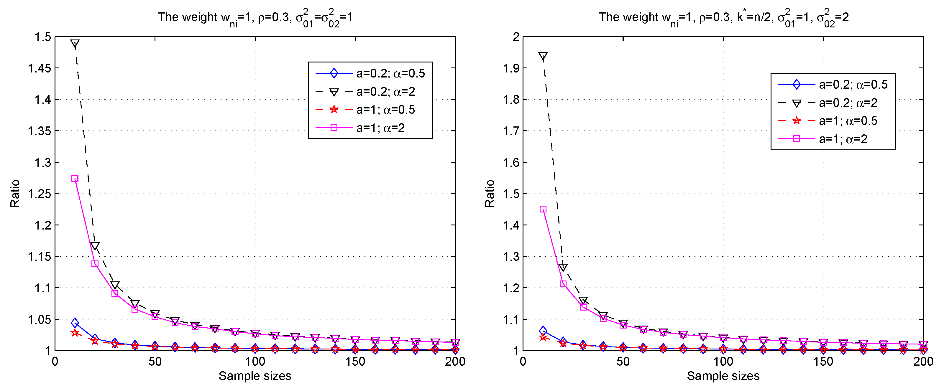
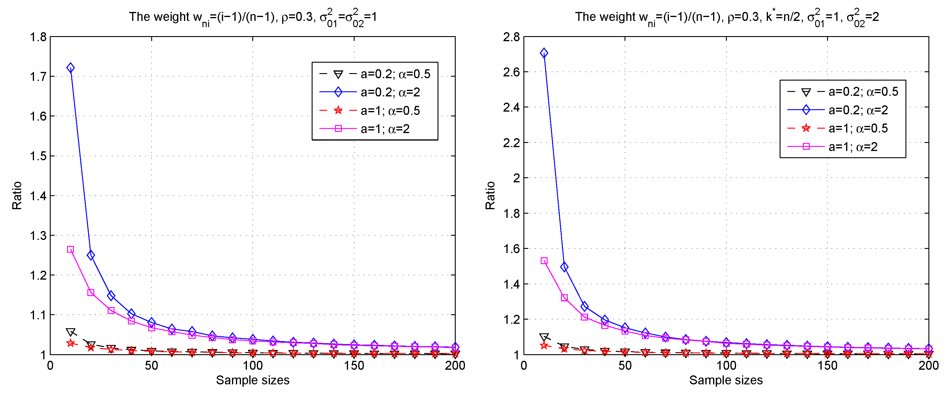
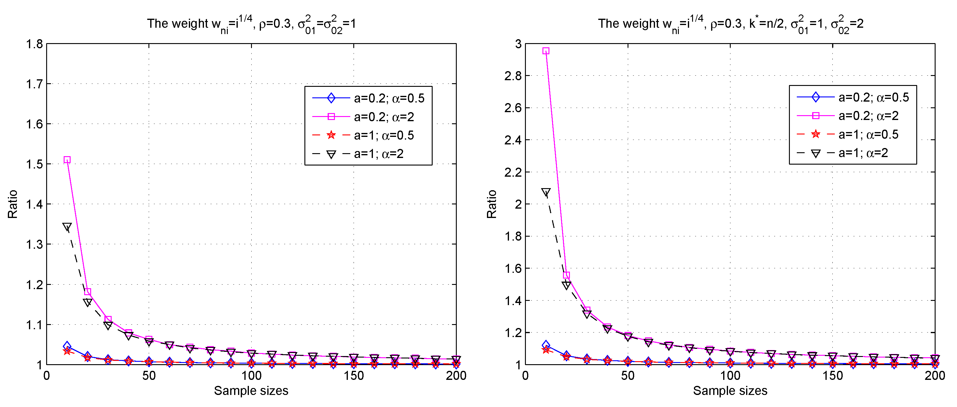
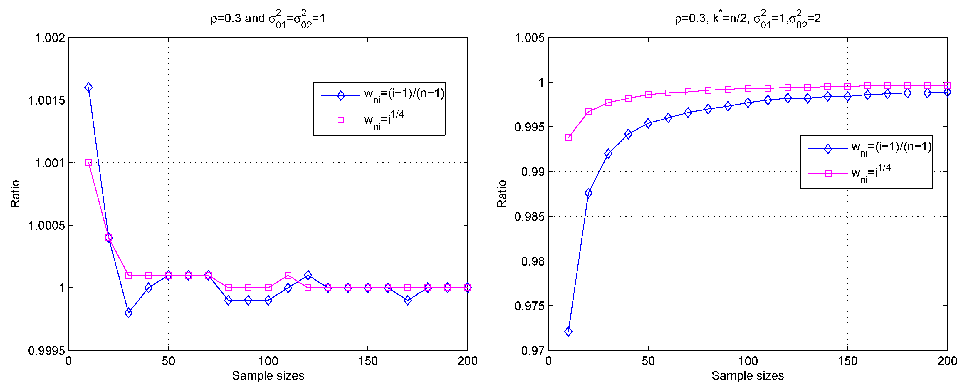
First, we do simulate (16). For all a > 0 and α > 0 , it has ( a + E X n ) α 0 as n , by the fact that E X n as n . So we use MATLAB software to obtain the empirical values for the “ratio” E ( a + X n ) α ( a + E X n ) α in (16) by repeating 10000 experiments and obtain the Figure 1, Figure 2, Figure 3 and Figure 4 The label of y-axis “ratio” is empirical values of (16) and the label of x-axis “sample sizes” is the number of sample n. For ρ = 0.3 and σ 01 2 = σ 02 2 = 1 (or k = n / 2 , σ 01 2 = 1 , σ 02 2 = 2 ), we take n = 10 , 20 , 30 , , 200 , a = 0.2 , 1 and α = 0.5 , 2 , and obtain the results of Figure 1, Figure 2, Figure 3 and Figure 4 for the weighted cases (C.1)–(C.4), respectively.
By Figure 1, Figure 2, Figure 3 and Figure 4, it can be found that the ratio E ( a + X n ) α ( a + E X n ) α 1 for all a > 0 and α > 0 , since it is guaranteed by Jensen’s inequality. As the sample n increases, the ratio E ( a + X n ) α ( a + E X n ) α decreases to one. So, the results of Figure 1, Figure 2, Figure 3 and Figure 4 are agreed with formulas of (5) and (7).
Second, we do the simulation for (17). It can be seen that E ( X n Y n ) / E X n E Y n = 1 under the equal weight cases of (C.1) and (C.2). So we do the simulation E ( X n Y n ) / E X n E Y n under the unequal weight cases of (C.3) and (C.4), and obtain Figure 5.
In Figure 5, the label of y-axis “ratio” is empirical values of (17) and the label of x-axis “sample sizes” is the number of sample n taking values n = 10 , 20 , 30 , , 200 . By Figure 5, the ratio E ( X n Y n ) / E X n E Y n goes to one as the sample n increases, which agrees with (13).
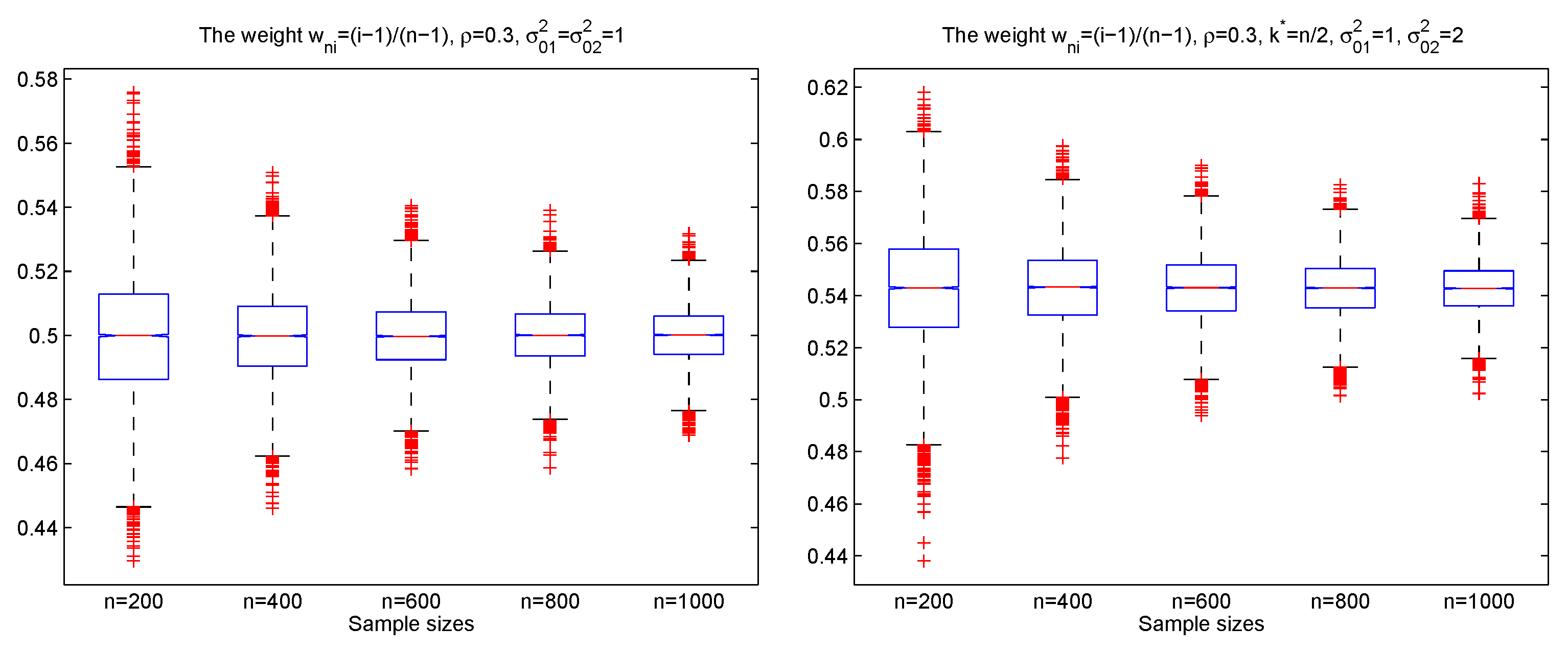
Third, we do some box plots of X n / Y n with the weight case of (C.3). If σ 01 2 = σ 02 2 = 1 in (14), then it is easy to check
E X n E Y n = i = 1 n i 1 n 1 E Z i i = 1 n E Z i = 1 2 .
Let x denote the largest integer not exceeding x. Likewise, we take k = n 2 , σ 01 2 = 1 , σ 02 2 = 2 and obtain that
E X n E Y n 5 2 2 4 0.5429 , as n .
Thus, we take ρ = 0.3 , n = 200 , 400 , , 1000 , σ 01 2 = σ 02 2 = 1 (or k = n / 2 and σ 01 2 = 1 , σ 02 2 = 2 ) and obtain the box plots in Figure 6, by repeating 10000 experiments.
By Figure 6, it is easy to see that the results are agreed with (18) and (19), respectively.

4. Conclusions

On one hand, by taking max 1 i n w n i = O ( 1 ) (i.e., γ = 0 ) in Theorems 1 and 2, one can obtain the results of (5), (7) and (8) with γ = 0 , which imply Theorems 2.1 and 2.2 of Li et al. [13] for nonnegative WOD sequences. Obviously, the condition (A.2) is weaker than the one of max 1 i n w n i = O ( 1 ) . So Theorems 1 and 2 generalize and improve the results of Li et al. [13]. On the other hand, independent sequence is a m-WOD sequence with g ( n ) = 1 . So by taking max 1 i n w n i = O ( 1 ) (i.e., λ = 0 ) and β = 0 in Theorem 3, we have (10) with λ = 0 and β = 0 , which implies Theorem 2.3 of Yang et al. [12] for nonnegative independent sequences. Furthermore, by using Theorems 2 and 3, we obtain Corollary 1 which does not contain the parameter a. It can be easy to use in practice (for example change-point detection). In addition, we also do some simulations to check our results such as E ( a + X n ) α ( a + E X n ) α 1 and E ( X n Y n ) / E X n E Y n 1 based on the different weight cases.

5. Proofs of Main Results

Lemma 1.
(Wang et al. [26] [Proposition 1.1]) Let { Z n , n 1 } be WUOD (WLOD) with dominating coefficients g u ( n ) , n 1 ( g l ( n ) , n 1 ) . If { f n ( · ) , n 1 } are nondecreasing, then { f n ( Z n ) , n 1 } are still WUOD (WLOD) with dominating coefficients g u ( n ) , n 1 ( g l ( n ) , n 1 ) ; if { f n ( · ) , n 1 } are nonincreasing, then { f n ( Z n ) , n 1 } are WLOD (WUOD) with dominating coefficients g l ( n ) , n 1 ( g u ( n ) , n 1 ) .
Corollary 2.
Let { Z n , n 1 } be a sequence of m-WOD random variables. If { f n ( · ) , n 1 } are nondecreasing (nonincreading) functions, then { f ( Z n ) , n 1 } are also m-WOD random variables with same dominating coefficients.
Proof of Corollary 2.
According to the definition of m-WOD, a sequence of m-WOD { Z n , n 1 } can decompose to m sequences of WOD, i.e. { Z 1 , Z 1 + m , Z 1 + 2 m , } , { Z 2 , Z 2 + m , Z 2 + 2 m , } , , { Z m , Z 2 m , Z 3 m , } . Then, by Lemma 1, the sequences { f ( Z 1 ) , f ( Z 1 + m ) , f ( Z 1 + 2 m ) , } , { f ( Z 2 ) , f ( Z 2 + m ) , f ( Z 2 + 2 m ) , } , , { f ( Z m ) , f ( Z 2 m ) , f ( Z 3 m ) , } are also WOD sequence with same dominating coefficients. Thus, by the definition of m-WOD again, { f ( Z n ) , n 1 } are also m-WOD random variables with same dominating coefficients. □
Lemma 2.
(Wang et al. [28] [Corollary 2.3]) Let q 2 and { Z n , n 1 } be a mean zero sequence of WOD random variables with dominating coefficient g ( n ) = max { g u ( n ) , g l ( n ) } and E | Z n | q < for all n 1 . Then for all n 1 , there exist positive constants C 1 ( q ) and C 2 ( q ) depending only on q such that
E | i = 1 n Z i | q C 1 ( q ) i = 1 n E | Z i | q + C 2 ( q ) g ( n ) i = 1 n E Z i 2 q / 2 .
Corollary 3.
Let q 2 and { Z n , n 1 } be a mean zero sequence of m-WOD random variables with dominating coefficient g ( n ) = max { g u ( n ) , g l ( n ) } and E | Z n | q < for all n 1 . Then for all n 1 , there exist a positive constant C ( m , q ) depending only on m and q such that
E | i = 1 n Z i | q C ( m , q ) i = 1 n E | Z i | q + g ( n ) i = 1 n E Z i 2 q / 2 .
Proof of Corollary 3.
By the definition of m-WOD, the sums of m-WOD can be written as
S n = i = 1 n Z i = j = 1 m i = 1 i j Z t i ( j ) ,
where i = 1 i j Z t i ( j ) are the sums of WOD, 1 j m . Then, by C r inequality and (9) in Lemma 2, it is easy to establish that
E | S n | q m q 1 j = 1 m E | i = 1 i j Z t i ( j ) | q m q 1 j = 1 m C 1 ( q ) i = 1 i j E | Z t i ( j ) | q + C 2 ( q ) g ( n ) i = 1 i j E ( Z t i ( j ) ) 2 q / 2 m q C 1 ( q ) i = 1 n E | Z i | q + C 2 ( q ) g ( n ) i = 1 n E ( Z i ) 2 q / 2 C ( m , q ) i = 1 n E | Z i | q + g ( n ) i = 1 n E Z i 2 q / 2 .
So the proof of (21) is finished. □
Proof of Theorem 1.
The proof is similar to the one of Theorem 2.1 in Li et al. [13], where Li et al. [13] consider WOD case with weight max 1 i n w n i = O ( 1 ) . In this paper, we consider general case (A.2) and give the key parts of proofs. By Jensen’s inequality, we have E ( a + X n ) α ( a + E X n ) α for all a > 0 and α > 0 . Thus, in order to prove (5), we only have to show that for δ ( 0 , 1 ) ,
lim   sup n { ( a + E X n ) α E ( a + X n ) α } ( 1 δ ) α ,
(or see Li et al. [13]). By (A.4), there exist a n ( δ ) > 0 such that for all δ ( 0 , 1 ) and
i = 1 n w n i E [ Z i I ( Z i > μ n s ) ] δ 4 i = 1 n w n i E Z i , n n ( δ ) .
We can break E ( a + X n ) α into two formulas:
E ( a + X n ) α : = Q 1 + Q 2 ,
where
Q 1 = E [ ( a + X n ) α I ( U n μ n δ μ n ) ] , Q 2 = E [ ( a + X n ) α I ( U n > μ n δ μ n ) ] ,
U n = i = 1 n w n i [ Z i I ( Z i μ n s ) + μ n s I ( Z i > μ n s ) ] .
Since X n U n , we obtain Q 2 E [ ( a + X n ) α I ( X n > μ n δ μ n ) ] ( a + μ n δ μ n ) α . So, by (A.3), we establish
lim   sup n { ( a + E X n ) α Q 2 } lim   sup n { ( a + μ n ) α ( a + μ n δ μ n ) α } = ( 1 δ ) α .
It follows from (23) that | μ n E U n | δ μ n / 2 for all n n ( δ ) . Denote Z n , i = w n i [ Z i I ( Z i μ n s ) + μ n s I ( Z i > μ n s ) ] , 1 i n . So, by Corollary 2, { Z n , i E Z n , i , 1 i n } are also mean zero m-WOD random variables with dominating coefficient g ( n ) . Thus, by Markov’s inequality, Corollary 3 and C r inequality, it has that for all q > 2 and n n ( δ ) ,
Q 1 = E [ ( a + X n ) α I ( U n μ n δ μ n ) ] a α P ( U n μ n δ μ n ) a α P ( | E U n U n | δ μ n / 2 ) 2 q C 1 ( m , q ) δ q μ n q i = 1 n E | Z n , i | q + g ( n ) ( i = 1 n E Z n , i 2 ) q / 2 C 2 ( m , q ) δ q μ n q i = 1 n w n i q [ E ( Z i q I ( Z i μ n s ) ) + μ n s q E I ( Z i > μ n s ) ] + C 3 ( m , q ) δ q μ n q g ( n ) i = 1 n w n i 2 [ E ( Z i 2 I ( Z i μ n s ) ) + μ n 2 s E I ( Z i > μ n s ) ] q / 2 C 2 ( m , q ) ( max 1 i n w n i ) q 1 δ q μ n q μ n s ( q 1 ) i = 1 n w n i [ E ( Z i I ( Z i μ n s ) ) + E ( Z i I ( Z i > μ n s ) ) ] + C 3 ( m , q ) ( max 1 i n w n i ) q / 2 δ q μ n q g ( n ) μ n s i = 1 n w n i [ E ( Z i I ( Z i μ n s ) ) + E ( Z i I ( Z i > μ n s ) ) ] q / 2 = : I n 1 + I n 2 .
If γ < 0 , then by the conditions (A.1)–(A.3) and (26) that
I n 1 + I n 2 C 4 ( m , q ) δ q μ n q [ μ n s ( q 1 ) μ n + μ n β ( μ n s μ n ) q / 2 ] = C 4 ( m , q ) δ q [ μ n ( q 1 ) ( 1 s ) + μ n β q 2 ( 1 s ) ] .
Since q > 2 , it has q 1 > q 2 . We take q > max { 2 , 2 ( α + β ) / ( 1 s ) } in (27) and obtain that
lim   sup n { ( a + E X n ) α Q 1 } lim   sup n { ( a + μ n ) α C 5 ( m , q ) δ q [ μ n ( q 1 ) ( 1 s ) + μ n β q 2 ( 1 s ) ] } = 0 .
Similarly, if 0 γ < 1 2 ( 1 s ) , then by the conditions (A.1)–(A.3) and (26) that
I n 1 + I n 2 C 6 ( m , q ) δ q μ n q [ μ n γ ( q 1 ) μ n s ( q 1 ) μ n + μ n γ q / 2 μ n β ( μ n s μ n ) q / 2 ] C 7 ( m , q ) δ q [ μ n γ ( q 1 ) ( q 1 ) ( 1 s ) + μ n γ ( q 1 ) + β q 2 ( 1 s ) ] .
In view of 0 γ < 1 2 ( 1 s ) , 0 < s < 1 , α > 0 and β 0 , if q > max { 2 , α + β 1 2 ( 1 s ) γ } , then
q ( γ 1 2 ( 1 s ) ) < α + β 1 2 ( 1 s ) γ ( γ 1 2 ( 1 s ) ) = α β α β + γ ,
which implies that
γ ( q 1 ) + β q 2 ( 1 s ) + α < 0 .
So we take q > max { 2 , α + β 1 2 ( 1 s ) γ } in (29) and obtain that
lim   sup n { ( a + E X n ) α Q 1 } lim   sup n { ( a + μ n ) α C 8 ( m , q ) δ q [ μ n γ ( q 1 ) ( q 1 ) ( 1 s ) + μ n γ ( q 1 ) + β q 2 ( 1 s ) ] } = 0 .
So, by (24), (25), (28) and (30), (22) holds true. □
Proof of Theorem 2.
By Taylor expansion, it can be checked that
E 1 ( a + X n ) α = 1 ( a + E X n ) α + α ( α + 1 ) 2 E ( X n E X n ) 2 ( a + ξ n ) α + 2 ,
where ξ n lies between X n and μ n . Next, we will verify that
E ( X n E X n ) 2 ( a + ξ n ) α + 2 = O 1 ( a + E X n ) α + 1 2 γ 2 β / r ,
where γ + 2 β / r < 1 and r > 2 . It is easy to see that
E ( X n E X n ) 2 ( a + ξ n ) α + 2 = E ( X n E X n ) 2 ( a + ξ n ) α + 2 I ( X n > μ n ) + E ( X n E X n ) 2 ( a + ξ n ) α + 2 I ( X n μ n ) .
On the one hand, for some r > 2 , it can be argued by Corollary 3, (6) and (A.2) that
E ( X n E X n ) 2 ( a + ξ n ) α + 2 I ( X n > μ n ) 1 ( a + μ n ) α + 2 E ( X n E X n ) 2 1 ( a + μ n ) α + 2 ( E | X n E X n | r ) 2 / r = 1 ( a + μ n ) α + 2 E | i = 1 n w n i ( Z i E Z i ) | r 2 / r C 1 ( m , r ) ( a + μ n ) α + 2 i = 1 n w n i r E | Z i E Z i | r + g ( n ) i = 1 n w n i 2 Var ( Z i ) r / 2 2 / r C 1 ( m , r ) ( max 1 i n w n i ) 2 ( a + μ n ) α + 2 i = 1 n E | Z i E Z i | r + g ( n ) i = 1 n Var ( Z i ) r / 2 2 / r C 2 ( m , r ) ( E X n ) 2 γ + 1 + 2 β / r ( a + E X n ) α + 2 = O 1 ( a + E X n ) α + 1 2 γ 2 β / r ,
where 2 γ + 2 β / r < 1 .
On the other hand, for some r > 2 , by the proof of (34), it can be found that
E ( X n E X n ) 2 ( a + ξ n ) α + 2 I ( X n μ n ) E ( X n E X n ) 2 ( a + X n ) α + 2 [ E | X n E X n | r ] 2 / r [ E ( a + X n ) ( α 2 ) r r 2 ] r 2 r ( by H ö lder inequality ) C 1 ( m , r ) E | i = 1 n w n i ( Z i E Z i ) | r 2 / r [ ( a + E X n ) ( α 2 ) r r 2 ] r 2 r ( by Theorem 2.1 ) = O 1 ( a + E X n ) α + 1 2 γ 2 β / r ,
where 2 γ + 2 β / r < 1 . Thus, (32) follows from (33) to (35). Combining (31) with (32), we obtain the result of (7) with γ + 2 β / r < 1 .
Last, similar to the proof of (2.3) in Li et al. [13], by (31) and (32), one can obtain that for all a > 0 and α > 1 ,
E X n ( a + X n ) α = 1 ( a + E X n ) α 1 + O 1 ( a + E X n ) α 2 γ 2 β / r a ( a + E X n ) α + O 1 ( a + E X n ) α + 1 2 γ 2 β / r = E X n ( a + E X n ) α + O 1 ( a + E X n ) α 2 γ 2 β / r .
Hence, by (36), (8) holds true. □
Proof of Theorem 3.
The proof is similar to the one of Theorem 2.3 in Yang et al. [12], where Yang et al. [12] consider the independent case and weight condition max 1 i n w n i = O ( 1 ) . In this paper, weight condition (B.2) is very weak. So we give the complete proofs here. By bivariate Taylor expansion, one can establish that
E X n a + Y n = E X n a + E Y n E ( X n E X n ) ( Y n E Y n ) η n 2 + E ξ n ( Y n E Y n ) 2 η n 3 : = E X n a + E Y n + E H n 1 + E H n 2 ,
where ξ n lies between X n and E X n , η n lies between a + Y n and a + E Y n , and H n 1 : = ( X n E X n ) ( Y n E Y n ) η n 2 , H n 2 : = ξ n ( Y n E Y n ) 2 η n 3 . Next, we will verify that
E | H n 1 | = O ( 1 ( a + E Y n ) 1 λ β / 2 ) and E | H n 2 | = O ( 1 ( a + E Y n ) 1 λ β / 2 ) ,
where λ β / 2 < 1 . It follows from (B.2) that
E X n = i = 1 n w n i E Z i max 1 i n w n i i = 1 n E Z i C 1 ( E Y n ) 1 + λ .
By Corollary 3 and conditions (B.1) and (B.5), one can check that
E ( X n E X n ) 4 C 1 ( m , 4 ) ( max 1 i n w n i ) 4 i = 1 n E ( Z i E Z i ) 4 + g ( n ) i = 1 n Var ( Z i ) 2 C 2 ( m ) ( E Y n ) 2 + β + 4 λ .
E ( Y n E Y n ) 4 C 3 ( m , 4 ) i = 1 n E ( Z i E Z i ) 4 + g ( n ) i = 1 n Var ( Z i ) 2 C 4 ( m ) ( E Y n ) 2 + β ,
which implies
E ( X n E X n ) 2 [ E ( X n E X n ) 4 ] 1 / 2 C 5 ( m ) ( E Y n ) 1 + 2 λ + β / 2 ,
E ( Y n E Y n ) 2 [ E ( Y n E Y n ) 4 ] 1 / 2 C 6 ( m ) ( E Y n ) 1 + β / 2 .
Combining Hölder inequality with (42) and (43), we obtain that
E | H n 1 I ( a + Y n > a + E Y n ) | = E | ( X n E X n ) ( Y n E Y n ) η n 2 I ( a + Y n > a + E Y n ) | 1 ( a + E Y n ) 2 E | ( X n E X n ) ( Y n E Y n ) | 1 ( a + E Y n ) 2 [ E ( X n E X n ) 2 ] 1 / 2 [ E ( Y n E Y n ) 2 ] 1 / 2 C 1 ( m ) ( E Y n ) 1 + λ + β / 2 ( a + E Y n ) 2 = O ( 1 ( a + E Y n ) 1 λ β / 2 ) .
By Hölder inequality, (40), (41), (B.1), (B.3), (B.4), we have that
E | H n 1 I ( a + Y n a + E Y n ) | = E | ( X n E X n ) ( Y n E Y n ) η n 2 I ( a + Y n a + E Y n ) | E | ( X n E X n ) ( Y n E Y n ) ( a + Y n ) 2 | { E [ ( X n E X n ) 2 ( Y n E Y n ) 2 ] } 1 / 2 E 1 ( a + Y n ) 4 1 / 2 { [ E ( X n E X n ) 4 ] 1 / 2 [ E ( Y n E Y n ) 4 ] 1 / 2 } 1 / 2 E 1 ( a + Y n ) 4 1 / 2 C 1 ( m ) ( E Y n ) 1 + λ + β / 2 1 ( a + E Y n ) 4 1 / 2 ( by Theorem 2.1 with γ = 0 ) = O ( 1 ( a + E Y n ) 1 λ β / 2 ) .
Similarly, we apply Hölder inequality, (39) and (41), then obtain that
E | H n 2 I ( X n E X n , a + Y n a + E Y n ) | = E | ξ n ( Y n E Y n ) 2 η n 3 I ( X n E X n , a + Y n a + E Y n ) | E X n E ( Y n E Y n ) 2 ( a + Y n ) 3 E X n [ E ( Y n E Y n ) 4 ] 1 / 2 E 1 ( a + Y n ) 6 1 / 2 C 1 ( m ) ( E Y n ) 2 + λ + β / 2 1 ( a + E Y n ) 6 1 / 2 ( by Theorem 2.1 ) = O 1 ( a + E Y n ) 1 λ β / 2 .
It follows from (39) and (43) that
E | H n 2 I ( X n E X n , a + Y n > a + E Y n ) | = E | ξ n ( Y n E Y n ) 2 η n 3 I ( X n E X n , a + Y n > a + E Y n ) | E X n ( a + E Y n ) 3 E ( Y n E Y n ) 2 C 1 ( m ) ( E Y n ) 2 + λ + β / 2 ( a + E Y n ) 3 = O 1 ( a + E Y n ) 1 λ β / 2 .
It can be seen that
E | H n 2 I ( X n > E X n , a + Y n a + E Y n ) | = E | ξ n ( Y n E Y n ) 2 η n 3 I ( X n > E X n , a + Y n a + E Y n ) | E X n ( Y n E Y n ) 2 ( a + Y n ) 3 E | ( X n E X n ) ( Y n E Y n ) 2 ( a + Y n ) 3 | + E X n E ( Y n E Y n ) 2 ( a + Y n ) 3 : = K n 1 + K n 2 .
For K n 1 , by Hölder inequality, (40) and (41),
| K n 1 | { E [ | X n E X n | 4 / 3 | Y n E Y n | 8 / 3 ] } 3 / 4 E 1 ( a + Y n ) 12 1 / 4 C 1 { [ E ( X n E X n ) 4 ] 1 / 3 [ E ( Y n E Y n ) 4 ] 2 / 3 } 3 / 4 1 ( a + E Y n ) 3 ( by Theorem 2.1 ) C 2 ( m ) { [ ( E Y n ) 2 + 4 λ + β ] 1 / 3 [ ( E Y n ) 2 + β ] 2 / 3 } 3 / 4 1 ( a + E Y n ) 3 = O 1 ( a + E Y n ) 3 2 λ 3 4 β = O 1 ( a + E Y n ) 1 λ β 2 + 1 2 β 4 = O 1 ( a + E Y n ) 1 λ β 2 ,
since β 2 . Similarly, for K n 2 , by Hölder inequality, (39) and (41),
| K n 2 | E X n [ E ( Y n E Y n ) 4 ] 1 / 2 E 1 ( a + Y n ) 6 1 / 2 C 2 ( m ) ( E Y n ) 2 + λ + β / 2 1 ( a + E Y n ) 3 ( by Theorem 2.1 ) = O 1 ( a + E Y n ) 1 λ β / 2 .
In addition, we have by Hölder inequality, (39), (41)–(43) and β 4 that
E | H n 2 I ( X n > E X n , a + Y n > a + E Y n ) | = E | ξ n ( Y n E Y n ) 2 η n 3 I ( X n > E X n , a + Y n > a + E Y n ) | 1 ( a + E Y n ) 3 E [ X n ( Y n E Y n ) 2 ] 1 ( a + E Y n ) 3 E | ( X n E X n ) ( Y n E Y n ) 2 | + E X n ( a + E Y n ) 3 E ( Y n E Y n ) 2 1 ( a + E Y n ) 3 [ E ( X n E X n ) 2 ] 1 / 2 [ E ( Y n E Y n ) 4 ] 1 / 2 + E X n ( a + E Y n ) 3 E ( Y n E Y n ) 2 C 1 ( m ) ( a + E Y n ) 3 2 λ 3 4 β + C 2 ( m ) ( a + E Y n ) 1 λ β / 2 = O 1 ( a + E Y n ) 1 λ β / 2 .
Therefore, (38) follows from (44) to (51) immediately. Combining (37) with (38), the proof of (10) is completed. □
Proof of Corollary 1.
In view of (B.2), there exists a positive constant C such that
X n = i = 1 n w n i Z i max 1 i n w n i i = 1 n Z i C ( E Y n ) λ Y n : = C n Y n .
Then
X n 1 + Y n X n Y n C n + X n 1 + Y n ,
which implies
E X n 1 + Y n E X n Y n E C n + X n 1 + Y n .
By (10) in Theorem 3 with a = 1 , we establish that
E X n 1 + Y n = E X n 1 + E Y n + O 1 ( E Y n ) 1 λ β / 2 ,
where λ β / 2 < 1 . In addition, by (7) in Theorem 2 with a = 1 , α = 1 , γ = 0 and r = 4 , we obtain that
E 1 1 + Y n = 1 1 + E Y n + O 1 ( E Y n ) 2 β / 2 .
Thus, by (52), (55) and (56), it can be checked that
E C n + X n 1 + Y n = C n E 1 1 + Y n + E X n 1 + Y n = C n 1 1 + E Y n + O 1 ( E Y n ) 2 β / 2 + E X n 1 + E Y n + O 1 ( E Y n ) 1 λ β / 2 = E X n 1 + E Y n + C n 1 + E Y n + O C n ( E Y n ) 2 β / 2 + O 1 ( E Y n ) 1 λ β / 2 , = E X n 1 + E Y n + O 1 ( E Y n ) 1 λ β / 2 ,
where λ + β / 2 < 1 . Furthermore, in view of lim n E X n 1 + E Y n × E Y n E X n = 1 and (54)–(57), the proof of (12) is finished to prove. Last, by ( E Y n ) λ + β / 2 = o ( E X n ) and (54)–(57), we have that
E X n Y n / E X n E Y n = 1 + O ( E Y n ) λ + β / 2 E X n .
Thus, (13) is completely proved. □

Author Contributions

Supervision W.Y.; software H.F. and S.D.; writing—original draft preparation, H.F., X.L. and W.Y. All authors have read and agreed to the published version of the manuscript.

Funding

This research was funded by (11701004, 11801003), NSF of Anhui Province (1808085QA03, 1808085QA17, 1808085QF212) and Provincial Natural Science Research Project of Anhui Colleges (KJ2019A0006, KJ2019A0021).

Acknowledgments

The authors are deeply grateful to editors and anonymous referees for their careful reading and insightful comments. The comments led us to significantly improve the paper.

Conflicts of Interest

The authors declare no conflict of interest.

References

  1. Wu, T.J.; Shi, X.P.; Miao, B.Q. Asymptotic approximation of inverse moments of nonnegative random variables. Statist. Probab. Lett. 2009, 79, 1366–1371. [Google Scholar] [CrossRef]
  2. Garcia, N.L.; Palacios, J.L. On inverse moments of nonnegative random variables. Statist. Probab. Lett. 2001, 53, 235–239. [Google Scholar] [CrossRef]
  3. Kaluszka, M.; Okolewski, A. On Fatou-type lemma for monotone moments of weakly convergent random variables. Statist. Probab. Lett. 2004, 66, 45–50. [Google Scholar] [CrossRef]
  4. Jäntschi, L. Detecting extreme values with order statistics in samples from continuous distributions. Mathematics 2020, 8, 216. [Google Scholar] [CrossRef] [Green Version]
  5. Wang, X.J.; Hu, S.H.; Yang, W.Z.; Ling, N.X. Exponential inequalities and inverse moment for NOD sequence. Statist. Probab. Lett. 2010, 80, 452–461. [Google Scholar] [CrossRef]
  6. Sung, S.H. On inverse moments for a class of nonnegative random variables. J. Inequal. Appl. 2010, 2010, 823767. [Google Scholar] [CrossRef] [Green Version]
  7. Xu, M.; Chen, P.Y. On inverse moments for nonnegative NOD sequence. Acta Math. Sin. (Chin. Ser.) 2013, 55, 201–206. [Google Scholar]
  8. Horng, W.J.; Chen, P.Y.; Hu, T.C. On approximation for inverse moments of nonnegative random variables. J. Math. Stat. Oper. Res. (JMSOR) 2012, 1, 38–42. [Google Scholar] [CrossRef]
  9. Hu, S.H.; Wang, X.H.; Yang, W.Z.; Wang, X.J. A note on the inverse moment for the nonnegative random variables. Commun. Statist.-Theory Methods 2014, 43, 1750–1757. [Google Scholar] [CrossRef]
  10. Shi, X.P.; Wu, Y.H.; Liu, Y. A note on asymptotic approximations of inverse moments of nonnegative random variables. Statist. Probab. Lett. 2010, 80, 1260–1264. [Google Scholar] [CrossRef]
  11. Yang, W.Z.; Hu, S.H.; Wang, X.J. On the asymptotic approximation of inverse moment for nonnegative random variables. Commun. Statist.-Theory Methods 2017, 46, 7787–7797. [Google Scholar] [CrossRef]
  12. Yang, W.Z.; Shi, X.P.; Li, X.Q.; Hu, S.H. Approximations to inverse moments of double-indexed weighted sums. J. Math. Anal. Appl. 2016, 440, 833–852. [Google Scholar] [CrossRef]
  13. Li, X.Q.; Liu, X.; Yang, W.Z.; Hu, S.H. The inverse moment for widely orthant dependent random variables. J. Inequal. Appl. 2016, 2016, 161. [Google Scholar] [CrossRef] [Green Version]
  14. Shi, X.P.; Reid, N.; Wu, Y.H. Approximation to the moments of ratios of cumulative sums. Canad. J. Statist. 2014, 42, 325–336. [Google Scholar] [CrossRef]
  15. Wang, Y.B.; Cheng, D.Y. Basic renewal theorems for random walks with widely dependent increments. J. Math. Anal. Appl. 2011, 384, 597–606. [Google Scholar] [CrossRef] [Green Version]
  16. Hu, T.C.; Chiang, C.Y.; Taylor, R.L. On complete convergence for arrays of rowwise m-negatively associated random variables. Nonlinear Anal. 2009, 71, e1075–e1081. [Google Scholar] [CrossRef]
  17. Liu, L. Precise large deviations for dependent random variables with heavy tails. Statist. Probab. Lett. 2009, 79, 1290–1298. [Google Scholar] [CrossRef]
  18. Lehmann, E.L. Some concepts of dependence. Ann. Math. Stat. 1966, 37, 1137–1153. [Google Scholar] [CrossRef]
  19. Hu, T.Z. Negatively superadditive dependence of random variables with applications. Chin. J. Appl. Probab. Statist. 2000, 16, 133–144. [Google Scholar]
  20. Joag-Dev, K.; Proschan, F. Negative association of random variables with applications. Ann. Statist. 1983, 11, 286–295. [Google Scholar] [CrossRef]
  21. Bulinski, A.V.; Shaskin, A. Limit Theorems for Associated Random Fields and Related Systems; World Scientific: Singapore, 2007; pp. 1–20. [Google Scholar]
  22. Davidian, M.; Giltinan, D.M. Nonlinear Models for Repeated Measurement Data; Chapman and Hall: New York, NY, USA, 1995; pp. 16–60. [Google Scholar]
  23. Tomasz, J.; Kozubowskia, T.J.; Podgórski, K.; Rychlik, I. Multivariate generalized Laplace distribution and related random fields. J. Multivar. Anal. 2013, 113, 59–72. [Google Scholar]
  24. Ko, B.; Tang, Q. Sums of dependent nonnegative random variables with subexponential tails. J. Appl. Probab. 2008, 45, 85–94. [Google Scholar] [CrossRef] [Green Version]
  25. Yang, W.Z.; Zhao, Z.R.; Wang, X.H.; Hu, S.H. The large deviation results for the nonlinear regression model with dependent errors. TEST 2017, 26, 261–283. [Google Scholar]
  26. Wang, Y.B.; Cui, Z.L.; Wang, K.Y.; Ma, X.L. Uniform asymptotics of the fnite-time ruin probability for all times. J. Math. Anal. Appl. 2012, 390, 208–223. [Google Scholar] [CrossRef] [Green Version]
  27. Wang, K.Y.; Wang, Y.B.; Gao, Q.W. Uniform asymptotics of the fnite-time ruin probability of dependent risk model with a constant interest rate. Methodol. Comput. Appl. Probab. 2013, 15, 109–124. [Google Scholar] [CrossRef]
  28. Wang, X.J.; Xu, C.; Hu, T.C.; Volodin, A.I.; Hu, S.H. On complete convergence for widely orthant-dependent random variables and its applications in nonparametric regression models. TEST 2014, 23, 607–629. [Google Scholar]
  29. Yang, W.Z.; Liu, T.T.; Wang, X.J.; Hu, S.H. On the Bahadur Representation of sample quantiles for widely orthant dependent sequences. Filomat 2014, 28, 1333–1343. [Google Scholar] [CrossRef] [Green Version]
  30. Wang, X.J.; Hu, S.H. The consistency of the nearest neighbor estimator of the density function based on WOD samples. J. Math. Anal. Appl. 2015, 429, 497–512. [Google Scholar] [CrossRef]
  31. Shen, A.T.; Zhang, Y.; Xiao, B.Q.; Volodin, A. Moment inequalities for m-negatively associated random variables and their applications. Statist. Pap. 2017, 58, 911–928. [Google Scholar] [CrossRef]
  32. Wang, X.J.; Wu, Y.; Hu, S.H. Exponential probability inequality for m-END random variables and its applications. Metrika 2016, 79, 127–147. [Google Scholar] [CrossRef]
  33. Wu, Y.F.; Rosalsky, A.; Volodin, A. Some mean convergence and complete convergence theorems for sequences of m-linearly negative quadrant dependent random variables. Appl. Math. 2013, 58, 511–529. [Google Scholar] [CrossRef] [Green Version]
  34. Wu, Y.F.; Rosalsky, A.; Volodin, A. Erratum to Some mean convergence and complete convergence theorems for sequences of m-linearly negative quadrant dependent random variables. Appl. Math. 2017, 62, 209–211. [Google Scholar] [CrossRef]
  35. Ye, R.Y.; Xinsheng Liu, X.S.; Yu, Y.C. Pointwise optimality of wavelet density estimation for negatively associated biased sample. Mathematics 2020, 8, 176. [Google Scholar] [CrossRef] [Green Version]
  36. Hsu, D.A. Detecting shifts of parameter in gamma sequences with applications to stock price and air traffic flow analysis. J. Am. Statist. Assoc. 1979, 74, 31–40. [Google Scholar] [CrossRef]
  37. Inclán, C.; Tiao, G.C. Use of cumulative sums of squares for retrospective detection of changes of variance. J. Am. Statist. Assoc. 1994, 89, 913–923. [Google Scholar]
  38. Abbas, N.; Abujiya, M.A.R.; Riaz, M.; Mahmood, T. Cumulative sum chart modeled under the presence of outliers. Mathematics 2020, 8, 269. [Google Scholar] [CrossRef] [Green Version]
  39. Doukhan, P.; Lang, G. Evaluation for moments of a ratio with application to regression estimation. Bernoulli 2009, 15, 1259–1286. [Google Scholar] [CrossRef]
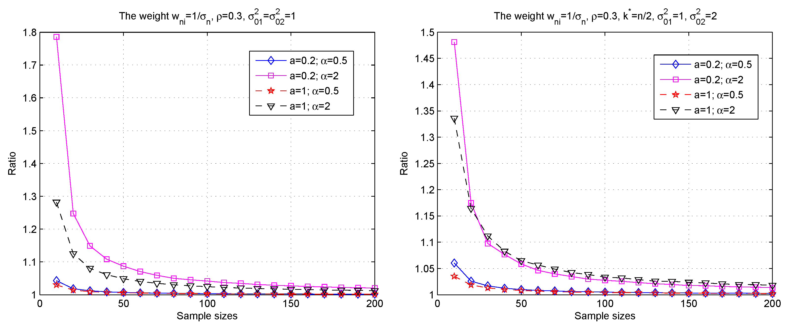
Figure 1. Empirical values of ratio E ( a + X n ) α ( a + E X n ) α for the weighted case w n i = 1 σ n , where ρ = 0.3 , σ 01 2 = σ 02 2 = 1 , or k = n / 2 and σ 01 2 = 1 , σ 02 2 = 2 .
Mathematics 08 00361 g001
Figure 2. Empirical values of ratio E ( a + X n ) α ( a + E X n ) α for the weighted case w n i = 1 , where ρ = 0.3 , σ 01 2 = σ 02 2 = 1 , or k = n / 2 and σ 01 2 = 1 , σ 02 2 = 2 .
Mathematics 08 00361 g002
Figure 3. Empirical values of ratio E ( a + X n ) α ( a + E X n ) α for the weighted case w n i = i 1 n 1 , where ρ = 0.3 , σ 01 2 = σ 02 2 = 1 , or k = n / 2 and σ 01 2 = 1 , σ 02 2 = 2 .
Mathematics 08 00361 g003
Figure 4. Empirical values of ratio E ( a + X n ) α ( a + E X n ) α for the weighted case w n i = i 1 / 4 , where ρ = 0.3 , σ 01 2 = σ 02 2 = 1 , or k = n / 2 and σ 01 2 = 1 , σ 02 2 = 2 .
Mathematics 08 00361 g004
Figure 5. Empirical values of ratio E ( X n Y n ) / E X n E Y n for the weighted cases w n i = i 1 n 1 and w n i = i 1 / 4 , ρ = 0.3 , σ 01 2 = σ 02 2 = 1 , or k = n / 2 and σ 01 2 = 1 , σ 02 2 = 2 .
Mathematics 08 00361 g005
Figure 6. Box plots of X n Y n for the weighted case w n i = i 1 n 1 , where ρ = 0.3 , σ 01 2 = σ 02 2 = 1 , or k = n / 2 and σ 01 2 = 1 , σ 02 2 = 2 .
Mathematics 08 00361 g006