Discrete Gompertz-G Family of Distributions for Over- and Under-Dispersed Data with Properties, Estimation, and Applications

Abstract

Alizadeh et al. introduced a flexible family of distributions, in the so-called Gompertz-G family. In this article, a discrete analogue of the Gompertz-G family is proposed. We also study some of its distributional properties and reliability characteristics. After introducing the general class, three special models of the new family are discussed in detail. The maximum likelihood method is used for estimating the family parameters. A simulation study is carried out to assess the performance of the family parameters. Finally, the flexibility of the new family is illustrated by means of four genuine datasets, and it is found that the proposed model provides a better fit than the competitive distributions.

1. Introduction

In probability and statistics, the Gompertz (Gz) distribution is a continuous probability distribution, named after Benjamin Gompertz. This distribution is a generalization of the exponential (Ex) distribution. The random variable T is said to have the Gz distribution with the shape parameter $\theta >0$and scale parameter $c>0$, if its cumulative distribution function (CDF) is given by

$$H(t;\theta ,c)=1-e^{-\frac{\theta }{c}(e^{ct}-1)};t>0.$$

(1)

The Gz distribution is often applied to describe the distribution of adult lifespans by demographers and actuaries. Related fields of science such as biology and gerontology also consider the Gz distribution for the analysis of survival. More recently, computer scientists have also started to model the failure rates of computer codes using the Gz distribution. In marketing science, it has been used as an individual-level simulation for customer lifetime value modeling. For more details, see Willemse et al. [1], Preston et al. [2], Melnikov and Romaniuk [3], Ohishi et al. [4], Bemmaor et al. [5], Cordeiro et al. [6], El-Bassiouny et al. [7,8,9], Alzaatreh et al. [10], Roozegar et al. [11], Mazucheli et al. [12], Eliwa et al. [13], among others.

Alizadeh et al. [14] introduced the Gz-G family based on a technique introduced by Alzaatreh et al. [10] in which a general form is used to generate a new family, named the transformed-transformer family. Thus, the random variable X is said to have the Gz-G family if its CDF is given by

$$\prod (y;\theta ,c,\mathit{\psi })=1-e^{-\frac{\theta }{c}\left\{{\left[1-G(y;\mathit{\psi })\right]}^{-c}-1\right\}};y>0,$$

(2)

where $\theta >0$ and $c>0$ are two additional parameters, $\mathit{\psi }$ is a vector of parameters ($1\times m;m=1,2,3,\dots$), and $G(y;\mathit{\psi })$ is the baseline CDF. The reliability function (RF) of the Gz-G family can be expressed as

$$\overline{\prod }(y;\theta ,c,\mathit{\psi })=e^{-\frac{\theta }{c}\left\{{\left[1-G(y;\mathit{\psi })\right]}^{-c}-1\right\}};y>0.$$

(3)

The probability density function (PDF) corresponding to Equation (2) can be written as

$$\pi (y;\theta ,c,\mathit{\psi })=\theta g(y;\mathit{\psi }){\left[\overline{G}(y;\mathit{\psi })\right]}^{-(c+1)}{e}^{-\frac{\theta }{c}\left\{{\left[1-G(y;\mathit{\psi })\right]}^{-c}-1\right\}};y>0,$$

(4)

where $g(y;\mathit{\psi })$ is the baseline PDF. Several authors used the technique of Alzaatreh et al. [14] to propose univariate and bivariate families; see for example, El-Morshedy and Eliwa [15], Eliwa and El-Morshedy [16,17], Alizadeh et al. [18], Eliwa et al. [19,20], El-Morshedy et al. [21], and the references cited therein.

Recently, discretizing continuous distributions has received much attention in the statistical literature. The discretization phenomenon generally arises when it becomes impossible or inconvenient to measure the life length of a product or a device on a continuous scale. Such situations may arise when the lifetimes need to be recorded on a discrete scale rather than on a continuous analogue. Therefore, several discrete distributions have been presented in the literature. See for example, Roy [22], Gómez-Déniz [23], Bebbington et al. [24], Nooghabi et al. [25], Nekoukhou et al. [26], Bakouch et al. [27], Nekoukhou and Bidram [28], Chandrakant et al. [29], Para and Jan [30], Mazucheli et al. [31], El-Morshedy et al. [17,20,32], Eliwa and El-Morshedy [33], among others. Although there are a number of discrete distributions in the statistical literature, there is still a lot of space left to develop new discretized distributions that are suitable under different conditions. Therefore, in this paper, we introduce a flexible discrete generator of distributions, in the so-called discrete Gz-G (DGz-G) family. Our reasons for introducing the DGz-G family are the following:

• To generate models with a negatively skewed, a positively skewed, or a symmetric shape;
• To define special models with all types of hazard rate function;
• To propose models which are appropriate for modeling both over- and under-dispersed data;
• To generate models for modeling both lifetime and counting datasets;
• To provide consistently better fits than other generated models under the same baseline distribution and other well-known models in the statistical literature.

The paper is organized as follows. In Section 2, the DGz-G family of distributions is defined. Some statistical and reliability properties of the DGz-G family are obtained in Section 3. In Section 4, three special models of the proposed family are discussed in detail. The family parameters are estimated by maximum likelihood method in Section 5. In Section 6, a simulation study is performed. The usefulness of the DGz-G family is illustrated by means of four genuine datasets, where we prove empirically that the DGz-G family outperforms some well-known distributions in Section 7. Section 8 offers some concluding remarks.

2. The DGz-G Family

Recall Equation (2), the random variable Z is said to have the DGz-G family if its CDF is given by

$$F_Z(z;p,c,\mathit{\psi })=1-p^{\frac{1}{c}\left\{{\left[1-G(z+1;\mathit{\psi })\right]}^{-c}-1\right\}};z\in {\mathbb{N}}_0,$$

(5)

where $p=e^{-\theta }$, $0<p<1$, $c>0$ and ${\mathbb{N}}_0=\left\{0,1,2,3,\dots \right\}$. Therefore, the RF of the DGz-G family can be represented as

$${\overline{F}}_Z(z;p,c,\mathit{\psi })=p^{\frac{1}{c}\left\{{\left[1-G(z+1;\mathit{\psi })\right]}^{-c}-1\right\}};z\in {\mathbb{N}}_0.$$

(6)

Let $Z_1,Z_2,\dots ,Z_n$ be non-negative independent and identically distributed (IID) integer valued random variables and $X=min(Z_1,Z_2,\dots ,Z_n)$, then X∼ DGz-G$(z;p^n,c,\mathit{\psi })$ family provided $Z_i$($i=1,2,\dots ,n$) ∼ DGz-G$(z;p,c,\mathit{\psi })$ family where

$${\overline{F}}_X(z;p,c,\mathit{\psi })=\prod _{i=1}^n\mathit{P}\left[Z_i\ge z\right]={\left(\mathit{P}\left[Z_1\ge z\right]\right)}^n=p^{\frac{n}{c}\left\{{\left[1-G(z+1;\mathit{\psi })\right]}^{-c}-1\right\}}.$$

(7)

Further, if ${\overline{F}}_{Z_i}\left(z\right)=p^{\frac{1}{c_i}\left\{{\left[1-G_i(z+1;\mathit{\psi })\right]}^{-c_i}-1\right\}},i=1,2$, then,

$${\overline{F}}_{Z_1}={\overline{F}}_{Z_2}\leftrightarrow \frac{log\left(1-G_1(z+1;\mathit{\psi })\right)}{log\left(1-G_2(z+1;\mathit{\psi })\right)}=1;\forall c_1=c_2=c$$

(8)

and

$${\overline{F}}_{Z_1}={\overline{F}}_{Z_2}\leftrightarrow c_2{\left[1-G_1(z+1;\mathit{\psi })\right]}^{-c_1}-c_1{\left[1-G_2(z+1;\mathit{\psi })\right]}^{-c_2}=c_1-c_2;\forall c_1\ne c_2.$$

(9)

The probability mass function (PMF) corresponding to Equation (5) can be expressed as

$$\begin{array}{cc}\hfill f_z(z;p,c,\mathit{\psi })& =\overline{F}\left(z\right)-\overline{F}(z+1)\hfill \\ \hfill & =p^{-\frac{1}{c}}\left[p^{\frac{1}{c}{\left[1-G(z;\mathit{\psi })\right]}^{-c}}-p^{\frac{1}{c}{\left[1-G(z+1;\mathit{\psi })\right]}^{-c}}\right];z\in {\mathbb{N}}_0.\hfill \end{array}$$

(10)

The hazard rate function (HRF) can be formulated as

$$h(z;p,c,\mathit{\psi })=1-p^{\frac{1}{c}\left\{{\left[1-G(z+1;\mathit{\psi })\right]}^{-c}-{\left[1-G(z;\mathit{\psi })\right]}^{-c}\right\}};z\in {\mathbb{N}}_0,$$

(11)

where $h(z;p,c,\mathit{\psi })=\frac{f_z(z;p,c,\mathit{\psi })}{{\overline{F}}_Z(z-1;p,c,\mathit{\psi })}$.

3. Different Statistical Properties

3.1. Quantile Function (QF)

For the DGz-G family, the qth QF, say $z_q$, is the solution of $F_Z\left(z_q\right)-q=0;z_q>0$, then

$$z_q=G^{-1}\left(1-{\left[1+\frac{clog(1-q)}{log\left(p\right)}\right]}^c\right)-1,$$

(12)

where $q\in (0,1)$ and $G^{-1}$represents the baseline QF. Setting $q=0.5$, we get the median of the DGz-G family.

3.2. Moments, Dispersion Index, Skewness, Kurtosis, and Cumulants

Assume non-negative random variable $Z\sim$ DGz-G$(z;p,c,\mathit{\psi })$ family, then the rth moment of Z can be expressed as

$$\begin{array}{cc}\hfill {\mu }_r^{\prime }& =\mathit{E}\left(Z^r\right)=\sum _{z=0}^{\infty }{z}^r{f}_z(z;p,c,\mathit{\psi })\hfill \\ \hfill & =\sum _{z=1}^{\infty }\left[z^r-{\left(z-1\right)}^r\right]{\overline{F}}_Z(z-1;p,c,\mathit{\psi })\hfill \\ \hfill & =p^{-\frac{1}{c}}\sum _{z=1}^{\infty }\left[z^r-{\left(z-1\right)}^r\right]p^{\frac{1}{c}{\left[1-G(z;\mathit{\psi })\right]}^{-c}}.\hfill \end{array}$$

(13)

Using Equation (13), the mean (${\mu }_1^{\prime }$) and variance (Var) can be respectively written as

$${\mu }_1^{\prime }=p^{-\frac{1}{c}}\sum _{z=1}^{\infty }{p}^{\frac{1}{c}{\left[1-G(z;\mathit{\psi })\right]}^{-c}}\mathrm{and}\mathit{Var}=p^{-\frac{1}{c}}\sum _{z=1}^{\infty }\left(2z-1\right)p^{\frac{1}{c}{\left[1-G(z;\mathit{\psi })\right]}^{-c}}-{\left({\mu }_1^{\prime }\right)}^2.$$

(14)

The dispersion index (DsI) is defined as variance to mean ratio, it indicates whether a certain model is suitable for over- or under-dispersed datasets, and is used widely in ecology as a standard measure for measuring clustering (over dispersion) or repulsion (under dispersion). If DsI $>1$ (DsI $<1$), the distribution is over-dispersed (under-dispersed). The DsI of the DGz-G family is given by

$$\mathit{DsI}=\frac{{\sum }_{z=1}^{\infty }\left(2z-1\right)p^{\frac{1}{c}{\left[1-G(z;\mathit{\psi })\right]}^{-c}}}{{\sum }_{z=1}^{\infty }{p}^{\frac{1}{c}{\left[1-G(z;\mathit{\psi })\right]}^{-c}}}-\sum _{z=1}^{\infty }{p}^{\frac{1}{c}{\left[1-G(z;\mathit{\psi })\right]}^{-c}}.$$

(15)

On the other hand, the moment generating function (MGF) can be represented as

$$\begin{array}{cc}\hfill M_Z\left(t\right)& =\sum _{z=0}^{\infty }{e}^{zt}{f}_z(z;p,c,\mathit{\psi })\hfill \\ \hfill & =p^{-\frac{1}{c}}\left[\sum _{z=0}^{\infty }{e}^{zt}{p}^{\Lambda (z;c)}-\sum _{z=0}^{\infty }{e}^{zt}{p}^{\Lambda (z+1;c)}\right]\hfill \\ \hfill & =p^{-\frac{1}{c}}[\left(p^{\Lambda (0;c)}+e^t{p}^{\Lambda (1;c)}+e^{2t}{p}^{\Lambda (2;c)}+e^{3t}{p}^{\Lambda (3;c)}+\dots \right)\hfill \\ \hfill & -\left(p^{\Lambda (1;c)}+e^t{p}^{\Lambda (2;c)}+e^{2t}{p}^{\Lambda (3;c)}+e^{3t}{p}^{\Lambda (4;c)}+\dots \right)]\hfill \\ \hfill & =p^{-\frac{1}{c}}\left[1+\sum _{z=1}^{\infty }\left(e^{zt}-e^{(z-1)t}\right)p^{\Lambda (z;c)}\right],\hfill \end{array}$$

(16)

where $\Lambda (z;c)=\frac{1}{c}{\left[1-G(z;\mathit{\psi })\right]}^{-c}$. The first four derivatives of Equation (16), with respect to t at $t=0$, yield the first four moments about the origin, i.e., $\mathit{E}\left(Z^r\right)=\frac{d^r}{d{t}^r}{M}_Z\left(t\right){|}_{t=0}$. Moreover, utilizing Equation (13) or (16), the skewness (Sk) and kurtosis (Ku) can be expressed as $\mathit{Sk}=({\mu }_3^{\prime }-3{\mu }_2^{\prime }{\mu }_1^{\prime }+2{\mu }_1^{\prime 3})/{\left(\mathit{Var}\right)}^{3/2}$ and $\mathit{Ku}=({\mu }_4^{\prime }-4{\mu }_3^{\prime }{\mu }_1^{\prime }+6{\mu }_2^{\prime }{\mu }_1^{\prime 2}-3{\mu }_1^{\prime 4})/{\left(\mathit{Var}\right)}^2$, respectively.

In probability theory, the cumulants, say $k_n$, of a probability model are a set of quantities that provide an alternative to the moments of a probability model. Because in some cases, theoretical treatments of problems in terms of cumulants are simpler than those using moments. The cumulant generating function (CGF) is the logarithm of the MGF. Thus, the $k_n$ can be recovered in terms of moments as follows:

$$k_n=\frac{d^n}{d{t}^n}log{M}_Z{\left(t\right)|}_{t=0};n=1,2,3,\dots .$$

(17)

Further, the cumulants are also related to the moments by the following recursion formula:

$$k_n={\mu }_n^{\prime }-\sum _{m=1}^{n-1}\left(\genfrac{}{}{0pt}{}{n-1}{m-1}\right){\mu }_{n-m}^{\prime }{k}_m.$$

(18)

The first cumulant is the mean, the second cumulant is the variance, and the third cumulant is the same as the third central moment. However, the fourth and higher-order cumulants are not equal to central moments.

3.3. Rényi Entropy

Entropy refers to the amount of uncertainty associated with a random variable Z. It has many applications in several fields such as econometrics, quantum information, information theory, survival analysis, and computer science (see Rényi [34]). The measure of variation of the uncertainty of the random variable Z can be expressed as

$$\begin{array}{cc}\hfill I_{\eta }\left(Z\right)& =\frac{1}{1-\eta }log\sum _{z=0}^{\infty }{f}_z^{\eta }(z;p,c,\mathit{\psi })\hfill \\ \hfill & =\frac{1}{1-\eta }\left\{-\frac{\eta }{c}logp+log\sum _{z=0}^{\infty }{\left[p^{\frac{1}{c}{\left[1-G(z;\mathit{\psi })\right]}^{-c}}-p^{\frac{1}{c}{\left[1-G(z+1;\mathit{\psi })\right]}^{-c}}\right]}^{\eta }\right\},\hfill \end{array}$$

(19)

where $\eta \in \left]0,\infty \right[$ and $\eta \ne 1$. The Shannon entropy can be defined by $\mathit{E}\left[-logf(Z;p,c,\mathit{\psi })\right]$. It is observed that the Shannon entropy can be calculated as a special case of the Rényi entropy when $\eta \to 1$.

3.4. Mean Time to Failure (MTTF), Mean Time between Failure (MTBF), and Availability (Av)

MTTF, MTBF, and Av are reliability terms based on methods and procedures for lifecycle predictions for a product. Customers often must include reliability data when determining what product to buy for their application. MTTF, MTBF, and Av are ways of providing a numeric value based on a compilation of data to quantify a failure rate and the resulting time of expected performance. In addition, in order to design and manufacture a maintainable system, it is necessary to predict the MTTF, MTBF, and Av. If $T\sim$ DGz-G$(t;p_1,c_1,{\mathit{\psi }}_1)$, then the MTBF is given as

$$\mathit{MTBF}=\frac{-t}{ln\left(p_1^{\frac{1}{c_1}\left\{{\left[1-G(t+1;{\mathit{\psi }}_1)\right]}^{-c_1}-1\right\}}\right)};t>0.$$

(20)

Whereas, if $T\sim$ DGz-G$(t;p_2,c_2,{\mathit{\psi }}_2)$, then the MTTF is given as

$$\mathit{MTTF}=p_2^{-\frac{1}{c_2}}\sum _{z=1}^{\infty }{p}_2^{\frac{1}{c_2}{\left[1-G(t;{\mathit{\psi }}_2)\right]}^{-c_2}};t>0.$$

(21)

The Av is considered as being the probability that the component is successful at time t, i.e., $\mathit{Av}=\frac{\mathit{MTTF}}{\mathit{MTBF}}$.

3.5. Order Statistics and L-Moment Statistics

3.5.1. Order Statistics (OS)

OS make their appearance in many areas of statistical theory and practice. Let $Z_1,Z_2,\dots$,$Z_n$ be a random sample from the DGz-G$(z;c,p,\mathit{\psi })$ family of distributions and let $Z_{1:n},Z_{2:n}$,...,$Z_{n:n}$ be their corresponding OS. Then, the CDF of the ith OS $Z_{i:n}$ for an integer value of z can be written as

$$\begin{array}{cc}\hfill F_{i:n}(z;p,c,\mathit{\psi })& =\sum _{k=i}^n\left(\begin{array}{c}n\\ k\end{array}\right){\left[F_i(z;p,c,\mathit{\psi })\right]}^k{\left[1-F_i(z;p,c,\mathit{\psi })\right]}^{n-k}\hfill \\ \hfill & =\sum _{k=i}^n\sum _{j=0}^{n-k}{(-1)}^j\left(\begin{array}{c}n\\ k\end{array}\right)\left(\begin{array}{c}n-k\\ j\end{array}\right){\left[F_i(z;p,c,\mathit{\psi })\right]}^{k+j}\hfill \\ \hfill & =\sum _{k=i}^n\sum _{j=0}^{n-k}\sum _{m=0}^{k+j}{\Delta }_{(n,k)}^{(m,j)}F(z;c,p^m,\mathit{\psi }),\hfill \end{array}$$

(22)

where ${\Delta }_{(n,k)}^{(m,j)}={(-1)}^{j+m}\left(\begin{array}{c}n\\ k\end{array}\right)\left(\begin{array}{c}n-k\\ j\end{array}\right)\left(\begin{array}{c}k+j\\ m\end{array}\right)$. The corresponding PMF of the ith OS can be expressed as

$$f_{i:n}(z;p,c,\mathit{\psi })=\sum _{k=i}^n\sum _{j=0}^{n-k}\sum _{m=0}^{k+j}{\Delta }_{(n,k)}^{(m,j)}f(z;p^m,c,\mathit{\psi }).$$

(23)

The uth moment of $Z_{i:n}$ can be written as

$${\Psi }_{i:n}^u=\mathit{E}\left(Z_{i:n}^u\right)=\sum _{z=0}^{\infty }\sum _{k=i}^n\sum _{j=0}^{n-k}\sum _{m=0}^{k+j}{\Delta }_{(n,k)}^{(m,j)}{z}^{u}f(z;p^m,c,\mathit{\psi }).$$

(24)

3.5.2. L-Moment (LM) Statistics

L-moments (LMs) obtain their name from their construction as linear combinations of OS. Hosking and Wallis [35] defined LMs as summaries of theoretical distribution and observed samples. Therefore, LM statistics are used for computing sample statistics for data at individual regions or for testing for homogeneity/heterogeneity of proposed groupings of sites. Let $Z\left(i\right|n)$ be ith largest observation in sample of size n, then the LMs can be take the form

$${\lambda }_r^{*}=\frac{1}{r}\sum _{s=0}^{r-1}{(-1)}^s\left(\begin{array}{c}r-1\\ s\end{array}\right)\mathit{E}\left(Z_{r-s:r}\right).$$

(25)

From Equation (25), we get ${\lambda }_1^{*}=\mathit{E}\left(Z_{1:1}\right)$, ${\lambda }_2^{*}=\frac{1}{2}\mathit{E}\left(Z_{2:2}+Z_{1:2}\right)$, ${\lambda }_3^{*}=\frac{1}{3}$[$\mathit{E}\left(Z_{3:3}-Z_{2:3}\right)-\mathit{E}\left(Z_{2:3}+Z_{1:3}\right)$], and ${\lambda }_4^{*}=\frac{1}{4}\left\{\mathit{E}\left[\left(Z_{4:4}-Z_{3:4}\right)+\left(Z_{2:4}-Z_{1:4}\right)\right]-2\mathit{E}\left(Z_{3:4}-Z_{2:4}\right)\right\}$. Then, we can define some statistical measures such as LM of mean, LM coefficient of variation, LM coefficient of Sk, and LM coefficient of ku in the form ${\lambda }_1^{*}$, $\frac{{\lambda }_2^{*}}{{\lambda }_1^{*}}$, $\frac{{\lambda }_3^{*}}{{\lambda }_2^{*}}$ and $\frac{{\lambda }_4^{*}}{{\lambda }_2^{*}}$, respectively.

4. Special Models

4.1. The DGz-Exponential (DGzEx) Distribution

Consider the CDF of the Ex distribution. Then, the PMF of the DGzEx distribution can be expressed as

$$f_Z(z;p,c,a)=p^{-\frac{1}{c}}\left[p^{\frac{1}{c}{e}^{acz}}-p^{\frac{1}{c}{e}^{ac(z+1)}}\right];z\in {\mathbb{N}}_0,$$

(26)

where $a>0$. The PMF in Equation (26) is log-concave for all values of the model parameters, where $\frac{f(z+1;p,c,a)}{f(z;p,c,a)}$ is a decreasing function in z for all values of the model parameters. Therefore, it is strongly unimodal, it has all its moments, and the HRFs are increasing. Figure 1 and Figure 2 show the PMF and HRF of the DGzEx distribution for various values of the parameters.

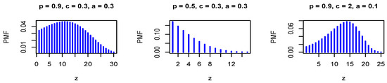
Figure 1. The probability mass function (PMF) of the discrete Gompertz exponential (DGzEx) distribution for different values of the parameters.

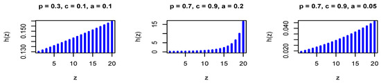
Figure 2. The hazard rate function (HRF) of the DGzEx distribution for different values of the parameters.

It is not possible to write the rth moment of the DGzE distribution in closed form, and therefore, we use Maple software to discuss some of its statistical properties. Other work such as Para and Jan [30], and Kundu and Nekoukhou [36] did not provide a closed form of the moments. Table 1 lists some descriptive statistics using the DGzEx model for different values of p and c with $a=0.2$.

Table 1. Some descriptive statistics using the DGzEx model.

Measure	$\mathit{c}\downarrow$$\mathit{p}\to$	$0.1$	$0.2$	$0.3$	$0.4$	$0.5$	$0.9$
	$0.5$	$1.3681$	$2.0006$	$2.6469$	$3.3775$	$4.2580$	$14.0712$
Mean	$0.7$	$1.2741$	$1.8431$	$2.4137$	$3.0479$	$3.7996$	$11.6368$
	$3.0$	$0.7217$	$1.0026$	$1.2632$	$1.5339$	$1.8345$	$4.3465$
	$0.5$	$2.4604$	$4.2059$	$6.2795$	$8.9082$	$12.3922$	$58.7099$
Var	$0.7$	$2.0555$	$3.3853$	$4.8947$	$6.7313$	$9.0693$	$35.6003$
	$3.0$	$0.6235$	$0.8678$	$1.0941$	$1.3258$	$1.5767$	$3.2289$
	$0.5$	$1.7985$	$2.1022$	$2.3723$	$2.6375$	$2.9103$	$4.1723$
DsI	$0.7$	$1.6133$	$1.8367$	$2.0278$	$2.2085$	$2.3869$	$3.0593$
	$3.0$	$0.8639$	$0.8655$	$0.8661$	$0.8643$	$0.8594$	$0.7429$
	$0.5$	$1.4129$	$1.2430$	$1.1112$	$0.9895$	$0.8668$	$0.1083$
Sk	$0.7$	$1.2922$	$1.1124$	$0.9756$	$0.8514$	$0.7281$	$-0.0081$
	$3.0$	$0.8051$	$0.5935$	$0.4465$	$0.3217$	$0.2042$	$-0.4138$
	$0.5$	$5.1652$	$4.5074$	$4.0441$	$3.6607$	$3.3204$	$2.2761$
Ku	$0.7$	$4.6191$	$4.0091$	$3.5963$	$3.2665$	$2.9841$	$2.2772$
	$3.0$	$2.8879$	$2.5828$	$2.4235$	$2.3266$	$2.2715$	$2.6635$

Regarding Table 1, it is clear that:

• The DGzEx distribution is a flexible distribution and can be used in modeling different types of datasets where
  • it is suitable for modeling over- and under-dispersed datasets where DsI $>(<)1$;
  • it is appropriate for modeling positive and negative skewness as well as symmetric datasets;
  • it can be used to model either platykurtic (Ku $<3$) or leptokurtic (Ku $>3$) data;
• The mean and Var increase whereas the Sk and Ku decrease for fixed values of a and c with $p⟶1$;
• The mean, Var, and Sk decrease for fixed values of a and p with $c⟶\infty$.

Table 2 shows the MTTF and entropy values for fixed values of $a=0.1$ and $\eta =0.5$ with $p⟶1$ and $c⟶\infty$.

Table 2. The mean time to failure (MTTF) and entropy using the DGzEx model.

Measure	$\mathit{c}\downarrow$$\mathit{p}\to$	$0.1$	$0.2$	$0.3$	$0.4$	$0.5$	$0.9$
MTTF	$0.9$	$2.8302$	$3.8848$	$4.9206$	$6.0536$	$7.3766$	$20.5048$
	$1.5$	$2.4574$	$3.3027$	$4.1084$	$4.9672$	$5.9455$	$14.8603$
	$3.0$	$1.8856$	$2.4649$	$2.9963$	$3.5449$	$4.1518$	$9.1905$
Entropy	$0.9$	$2.3866$	$2.6186$	$2.7914$	$2.9414$	$3.0824$	$3.7399$
	$1.5$	$2.2026$	$2.4043$	$2.5528$	$2.6803$	$2.7989$	$3.3373$
	$3.0$	$1.8870$	$2.0485$	$2.1655$	$2.2648$	$2.3561$	$2.7591$

According to Table 2, it is clear that the MTTF and entropy increase for fixed values of $a,c,$and $\eta$ with $p⟶1$. Whereas, for fixed values of $a,p,$and $\eta$ with $c⟶\infty$, the MTTF and entropy decrease.

4.2. The DGz-Weibull (DGzW) Distribution

Consider the CDF of the Weibull (W) distribution. Then, the PMF of the DGzW distribution can be expressed as

$$f_Z(z;p,c,a,b)=p^{-\frac{1}{c}}\left[p^{\frac{1}{c}{e}^{ac{z}^b}}-p^{\frac{1}{c}{e}^{ac{(z+1)}^b}}\right];z\in {\mathbb{N}}_0,$$

(27)

where $a,b>0$. The PMF in Equation (27) is log-concave for some values of the model parameters, where $\frac{f(z+1;p,c,a,b)}{f(z;p,c,a,b)}$ is a decreasing function in z for some values of the model parameters. Figure 3 and Figure 4 show the PMF and HRF of the DGzW distribution for various values of the parameters.

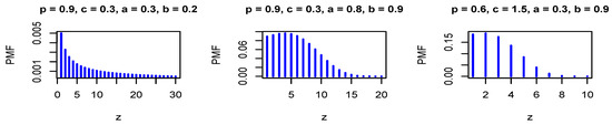
Figure 3. The PMF of the DGz-Weibull (DGzW) distribution for different values of the parameters.

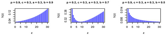
Figure 4. The HRF of the DGzW distribution for different values of the parameters.

It is immediate that the PMF is unimodal and the HRF can be either increasing, decreasing, or of bathtub shape. Hence, the parameters of the underlying distribution can be adjusted to suit most datasets. Like in the case of the DGzE distribution, it is not possible to write the rth moment in closed form, and consequently, Maple is used to explain some of the statistical properties of the DGzW distribution. Table 3 shows some descriptive statistics utilizing the DGzW distribution for various values of p and c with $a=0.5$ and $b=1.5$.

Table 3. Some descriptive statistics using the DGzW model.

Measure	$\mathit{c}\downarrow$$\mathit{p}\to$	$0.1$	$0.2$	$0.3$	$0.4$	$0.5$	$0.9$
	$0.1$	$0.3385$	$0.5337$	$0.7309$	$0.9518$	$1.2169$	$4.2810$
Mean	$0.5$	$0.2792$	$0.4375$	$0.5904$	$0.7538$	$0.9399$	$2.6171$
	$0.9$	$0.2350$	$0.3720$	$0.4996$	$0.6336$	$0.7843$	$2.0254$
	$0.1$	$0.2889$	$0.4583$	$0.6473$	$0.8820$	$1.1941$	$6.1147$
Var	$0.5$	$0.2188$	$0.3199$	$0.4166$	$0.5198$	$0.6375$	$1.5375$
	$0.9$	$0.1826$	$0.2538$	$0.3142$	$0.3784$	$0.4483$	$0.8329$
	$0.1$	$0.8533$	$0.8588$	$0.8857$	$0.9267$	$0.9813$	$1.4283$
DsI	$0.5$	$0.7839$	$0.7312$	$0.7056$	$0.6896$	$0.6783$	$0.5875$
	$0.9$	$0.7768$	$0.6822$	$0.6289$	$0.5971$	$0.5715$	$0.4113$
	$0.1$	$1.3392$	$1.0753$	$0.9492$	$0.8626$	$0.7874$	$0.2343$
Sk	$0.5$	$0.2959$	$0.8645$	$0.6725$	$0.5288$	$0.4058$	$-0.2801$
	$0.9$	$1.3032$	$0.7648$	$0.5483$	$0.4256$	$0.2959$	$-0.4358$
	$0.1$	$4.0792$	$3.6991$	$3.5429$	$3.4157$	$3.2796$	$2.3878$
Ku	$0.5$	$2.2544$	$2.7664$	$2.6085$	$2.4946$	$2.4198$	$2.4556$
	$0.9$	$2.8612$	$2.1388$	$2.2612$	$2.3467$	$2.2544$	$2.6264$

Regarding Table 3, it is clear that:

• The DGzW distribution is a flexible distribution and can be used for modeling various types of datasets where
  • it is suitable for modeling under- and over-dispersed datasets;
  • it is appropriate for modeling negative and positive skewness as well as symmetric datasets;
  • it can be used to model either platykurtic or leptokurtic data;
• The mean and Var increase for fixed values of $a,b$ and c with $p⟶1$;
• The mean and Var decrease for fixed values of $a,b$ and p with $c⟶\infty$.

Table 4 shows the MTTF and entropy values for fixed values of $a=b=\eta =0.5$ with $p⟶1$ and $c⟶\infty$.

Table 4. The MTTF and entropy using the DGzW model.

Measure	$\mathit{c}\downarrow$$\mathit{p}\to$	$0.1$	$0.2$	$0.3$	$0.4$	$0.5$	$0.9$
MTTF	$1.5$	$0.2582$	$0.5292$	$0.8624$	$1.2895$	$1.8597$	$10.6242$
	3	$0.0727$	$0.1752$	$0.3071$	$0.4770$	$0.7011$	$3.7762$
	5	$0.0058$	$0.0274$	$0.0680$	$0.1310$	$0.2221$	$1.5402$
Entropy	$1.5$	$1.0405$	$1.3979$	$1.6813$	$1.9365$	$2.1829$	$3.4507$
	3	$0.5078$	$0.7617$	$0.9747$	$1.1721$	$1.3662$	$2.3916$
	5	$0.1423$	$0.2903$	$0.4356$	$0.5815$	$0.7323$	$1.5874$

According to Table 4, it is clear that the MTTF and entropy increase for fixed values of $a,b,c,$and $\eta$ with $p⟶1$. Whereas, for fixed values of $a,b,p,$and $\eta$ with $c⟶\infty$, the MTTF and entropy decrease.

4.3. The DGz-Inverse Weibull (DGzIW) Distribution

Consider the CDF of the inverse Weibull (IW) distribution. Then, the PMF of the DGzIW distribution can be expressed as

$$f_Z(z;p,c,a,b)=p^{-\frac{1}{c}}\left[p^{\frac{1}{c}{\left(1-e^{-a{z}^{-b}}\right)}^{-c}}-p^{\frac{1}{c}{\left(1-e^{-a{(z+1)}^{-b}}\right)}^{-c}}\right];z\in {\mathbb{N}}_0,$$

(28)

where $a,b>0$. The PMF in Equation (28) is log-concave for some values of the model parameters. Figure 5 and Figure 6 show the PMF and HRF of the DGzIW distribution for various values of the parameters.

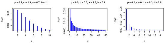
Figure 5. The PMF of the DGz-inverse Weibull (DGzIW) distribution for different values of the parameters.

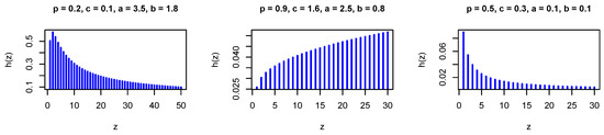
Figure 6. The HRF of the DGzIW distribution for different values of the parameters.

It is immediate that the PMF is decreasing, whereas the HRF can be either increasing, decreasing, or of unimodal shape. Hence, the parameters of the underlying distribution can be adjusted to suit most datasets.

5. Maximum Likelihood Estimation (MLE)

In this section, we estimate the unknown parameters of the DGz-G family using the maximum likelihood (ML) method. Suppose $Z_1,Z_2,\dots$,$Z_n$ is a random sample from the DGz-G family. Then, the log-likelihood function (L) can be expressed as

$$L=-\frac{1}{c}ln\left(p\right)+{\displaystyle \sum _{i=1}^n}ln\left(p^{\frac{1}{c}\left\{{\left[1-G(z_i;\mathit{\psi })\right]}^{-c}\right\}}-p^{\frac{1}{c}\left\{{\left[1-G(z_i+1;\mathit{\psi })\right]}^{-c}\right\}}\right).$$

(29)

The MLEs of the parameters $p,$$c,$ and $\mathit{\psi }$ can be derived by solving the nonlinear likelihood equations obtained by differentiating (Equation (29)). The components of the score vector, $\mathit{V}(p,c,\mathit{\psi })={(\frac{\partial L}{\partial p},\frac{\partial L}{\partial c},\frac{\partial L}{\partial \mathit{\psi }})}^T,$ are

$$V_p=\frac{-n}{cp}+\frac{1}{cp}{\displaystyle \sum _{i=1}^n}\frac{g_2\left(z_i\right)-g_2(z_i+1)}{g_1\left(z_i\right)},$$

(30)

$$V_c=\frac{-nln\left(p\right)}{c^2}-\frac{ln\left(p\right)}{c^2}{\displaystyle \sum _{i=1}^n}\frac{g_2\left(z_i\right)\left[cln(1-G(z_i;\mathit{\psi }))+1\right]-g_2(z_i+1)\left[cln(1-G(z_i+1;\mathit{\psi }))+1\right]}{g_1\left(z_i\right)}$$

(31)

and

$$V_{{\mathit{\psi }}_j}={\displaystyle \sum _{i=1}^n}\frac{g_2\left(z_i\right){\left[1-G(z_i;\mathit{\psi })\right]}^{-1}{\left[G(z_i;\mathit{\psi })\right]}_{{\mathit{\psi }}_j}-g_2(z_i+1){\left[1-G(z_i+1;\mathit{\psi })\right]}^{-1}{\left[G(z_i+1;\mathit{\psi })\right]}_{{\mathit{\psi }}_j}}{g_1\left(z_i\right)},$$

(32)

where ${\left[G(z_i;\mathit{\psi })\right]}_{{\mathit{\psi }}_j}=\partial G(z_i;\mathit{\psi })/\partial {\mathit{\psi }}_j$; $j=1,2,\dots ,m,$$g_1\left(z_i\right)=p^{\frac{1}{c}\left\{{\left[1-G(z_i;\mathit{\psi })\right]}^{-c}\right\}}-p^{\frac{1}{c}\left\{{\left[1-G(z_i+1;\mathit{\psi })\right]}^{-c}\right\}}$, and $g_2\left(z_i\right)=p^{\frac{1}{c}\left\{{\left[1-G(z_i;\mathit{\psi })\right]}^{-c}\right\}}\left\{{\left[1-G(z_i;\mathit{\psi })\right]}^{-c}\right\}.$ Setting the Equations (30)–(32) to zero and solving them, immediately yields the MLEs for the DGz-G family parameters. These equations cannot be solved analytically; therefore, an iterative procedure like Newton–Raphson is required to solve them numerically.

6. Simulation Results

In this section, we assess the performance of the MLE with respect to sample size n. The assessment is based on a simulation study which is describes in the following:

• Generate 1000 samples of size $n=$$20,23,26,\dots ,60$ from DGzEx$(0.1,1.5,0.8)$, DGzW($0.3,0.7,0.8,0.9$)
  and DGzIW($0.3,1.7,0.8,0.9$), respectively;
• Compute the MLEs for the 1000 samples, say ${\widehat{a}}_j$ and ${\widehat{b}}_j$ for $j=1,2,\dots ,1000$;
• Compute the biases and mean-squared errors (MSEs), where

  $$\mathrm{bias}(\alpha )=\frac{1}{1000}\sum _{j=1}^{1000}\left({\widehat{a}}_j-\alpha \right)\mathrm{and}\mathrm{MSE}(\alpha )=\frac{1}{1000}\sum _{j=1}^{1000}{\left({\widehat{a}}_j-\alpha \right)}^2.$$

The empirical results are shown in Figure 7, Figure 8, Figure 9, Figure 10, Figure 11 and Figure 12.

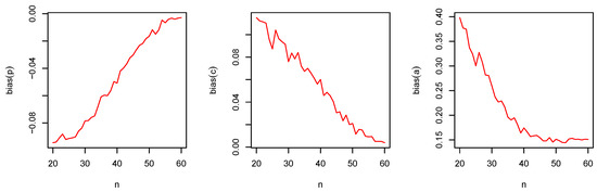
Figure 7. The bias of $\widehat{p},\widehat{c},$ and $\widehat{a}$ versus for the DGzEx$(0.1,1.5,0.8)$.

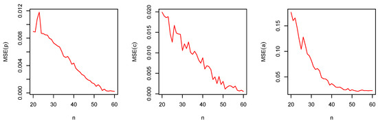
Figure 8. The MSE of $\widehat{p},\widehat{c},$ and $\widehat{a}$ versus for the DGzEx$(0.1,1.5,0.8)$.

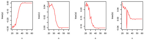
Figure 9. The bias of $\widehat{p},\widehat{c},$$\widehat{a},$ and $\widehat{b}$ versus for the DGzW($0.3,0.7,0.8,0.9$).

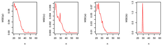
Figure 10. The MSE of $\widehat{p},\widehat{c},\widehat{a},$ and $\widehat{b}$ versus for the DGzW($0.3,0.7,0.8,0.9$).

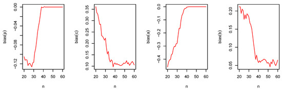
Figure 11. The bias of $\widehat{p},\widehat{c},\widehat{a},$ and $\widehat{b}$ versus for the DGzIW($0.3,1.7,0.8,0.9$).

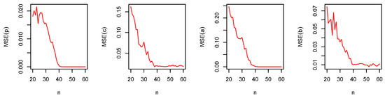
Figure 12. The MSE of $\widehat{p},\widehat{c},\widehat{a},$ and $\widehat{b}$ versus for the DGzIW($0.3,1.7,0.8,0.9$).

From Figure 7, Figure 8, Figure 9, Figure 10, Figure 11 and Figure 12, the following observations can be noted:

• The magnitude of bias always decreases to zero as $n\to \infty$;
• The MSEs always decrease to zero as $n\to \infty$. This shows the consistency of the estimators;
• Under the MLE method, the estimator of p is slightly negatively biased;
• The MLE method performs quite well for the parameters estimation.

We have presented results only for DGzEx$(0.1,1.5,0.8)$, DGzW($0.3,0.7,0.8,0.9$), and DGzIW($0.3,1.7,0.8,0.9$). However, the results are similar for other choices for $p,c,a,$ and b.

7. Data Analysis

In this section, we illustrate the empirical importance of the DGzW, DGzEx, and DGzIW distributions using four applications to real data. The fitted models are compared using some criteria, namely, L, Akaike information criterion (AIC), correct Akaike information criterion (CAIC), Chi-square (${\chi }^2$) with degree of freedom (d.f) and its p-value, Kolmogorov-Smirnov (K-S) and its p-value. We shall compare the DGzW, DGzEx, and DGzIW distributions with some competitive models described in Table 5.

Table 5. The competitive models of the DGzW, DGzEx, and DGzIW distributions.

Distribution	Abbreviation	Author(s)
Discrete Weibull	DW	Nakagawa and Osaki [37]
Exponentiated discrete Weibull	EDW	Nekoukhou and Bidram [28]
Discrete inverse Weibull	DIW	Jazi et al. [38]
Discrete exponential	DEx	Gómez-Déniz [23]
Discrete generalized exponential type II	DGEx-II	Nekoukhou et al.  [26]
Discrete Rayleigh	DR	Roy [22]
Discrete inverse Rayleigh	DIR	Hussain and Ahmad [39]
Discrete Lindley	DLi	Gómez-Déniz and Calderín-Ojeda  [40]
Exponentiated discrete Lindley	EDLi	El-morshedy et al. [41]
Discrete Lindley type II	DLi-II	Hussain et al. [42]
Discrete log-logistic	DLLc	Para and Jan [43]
Discrete Lomax	DLo	Para and Jan [44]
Two-parameter discrete Burr type XII	DB-XII	Para and Jan [44]
Discrete Pareto	DPa	Krishna and Pundir [45]
Negative binomial	NvBi	Dougherty [46]
Poisson	Poi	Poisson [47]

7.1. Dataset 1

This data represents the failure times (in weeks) of 50 devices put on a life test (see Bebbington et al. [24]). We compare the fits of the DGzW distribution with some competitive models, such as exponentiated discrete Weibull (EDW), discrete Weibull (DW), discrete inverse Weibull (DIW), discrete Lindley type II (DLi-II), exponentiated discrete Lindley (EDLi), discrete log-logistic (DLLc), and discrete Pareto (DPa). The MLEs with their corresponding standard errors (Std-er), and the goodness of fit statistics are reported in Table 6 and Table 7, respectively.

Table 6. The maximum likelihood estimations (MLEs) with their corresponding standard errors (Std-er) for Dataset 1.

Model ↓ Parameter →	p		c		a		b
	MLE	Std-er	MLE	Std-er	MLE	Std-er	MLE	Std-er
DGzW	$0.938$	$0.444$	$0.499$	$3.709$	$0.364$	$2.683$	$0.620$	$0.163$
EDW	$0.989$	$0.164$	$1.139$	$3.227$	$0.784$	$3.053$	−	−
DW	$0.981$	$0.011$	$1.023$	$0.131$	−	−	−	−
DIW	$0.018$	$0.013$	$0.582$	$0.061$	−	−	−	−
DLi-II	$0.969$	$0.005$	$0.058$	$0.027$	−	−	−	−
EDLi	$0.972$	$0.005$	$0.480$	$0.087$	−	−	−	−
DLLc	$1.0$	$0.321$	$0.439$	$0.062$	−	−	−	−
DPa	$0.739$	$0.032$	−	−	−	−	−	−

Table 7. The goodness of fit statistics for Dataset 1.

Statistic ↓ Model →	DGzW	EDW	DW	DIW	DLi-II	EDLi	DLLc	DPa
$-\mathit{L}$	$233.1$	$240.2$	$241.6$	$261.9$	$240.6$	$240.3$	$294.9$	$275.9$
AIC	$474.1$	$486.7$	$487.2$	$527.8$	$485.2$	$484.6$	$593.8$	$553.7$
CAIC	$474.9$	$487.2$	$487.5$	$528.1$	$485.4$	$484.8$	$594.0$	$553.8$
K-S	$0.161$	$0.195$	$0.187$	$0.258$	$0.186$	$0.195$	$0.535$	$0.335$
p-value	$0.149$	$0.045$	$0.061$	$0.0026$	$0.064$	$0.045$	$<0.001$	$<0.001$

Regarding Table 7, it is clear that the DW and DLi-II models work quite well for analyzing these data aside from the DGzW model (p-value $>0.05$). However, we always search for the best model to get the best evaluation of the data, and therefore, concerning the $-L$, AIC, CAIC, K-S, and p-values, we can say that the DGzW model provides the best fit among all the tested models because it has the smallest values of $-L$, AIC, CAIC, and K-S statistics, as well as having the highest p-value. Figure 13 and Figure 14 support the results of Table 7.

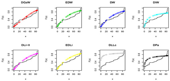
Figure 13. The estimated CDFs for Dataset 1.

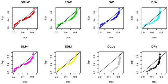
Figure 14. The probability-probability (P-P) plots for Dataset 1.

It is clear that the dataset plausibly came from the DW and DLi-II models. However, the the DGzW model is the best. Table 8 lists some statistics for Dataset 1 based on the DGzW parameters.

Table 8. Some statistics for Dataset 1.

Model	Mean	Var	DsI	Sk	Ku
DGzW	$30.4215$	$515.8454$	$16.9565$	$0.6867$	$2.5391$

Regarding Table 8, it is clear that these data suffer from over-dispersion phenomena. Moreover, these data are moderately skewed to the right: its right tail is longer and most of the distribution is to the left with platykurtic. The MTTF of these data equals $30.4215,$ whereas the entropyequals $2.3640$. Table 9 lists some numerical values of the reliability properties when using Dataset 1.

Table 9. Some reliability measures using Dataset 1.

Time $\downarrow$Measure →	RF	HRF	MTBF
2	$0.9595$	$0.0158$	$48.4225$
4	$0.9335$	$0.0146$	$58.2074$
6	$0.9099$	$0.0143$	$63.5477$
8	$0.8871$	$0.0144$	$66.8099$
10	$0.8648$	$0.0146$	$68.8551$
12	$0.8426$	$0.0149$	$70.1041$
14	$0.8205$	$0.0153$	$70.7972$
16	$0.7984$	$0.0158$	$71.0850$
18	$0.7763$	$0.0163$	$71.0684$
20	$0.7539$	$0.0168$	$70.8183$
22	$0.7315$	$0.0174$	$70.3866$
24	$0.7090$	$0.0181$	$69.8118$
26	$0.6865$	$0.0187$	$69.1241$
28	$0.6639$	$0.0194$	$68.3465$
30	$0.6411$	$0.0201$	$67.4975$

Regarding Table 9, it is clear that the RF decreases with $t\to \infty$. Further, the HRF is bathtub-shaped, whereas the MTBF has a unimodal shape.

7.2. Dataset 2

These data are reported in Lawless [48] and it gives the failure times for a sample of 15 electronic components in an acceleration life test. For this dataset, we compare the fits of the DGzEx distribution with some competitive models such as discrete exponential (DEx), Discrete generalized exponential type II (DGEx-II), discrete Rayleigh (DR), discrete inverse Rayleigh (DIR), discrete inverse Weibull (DIW), discrete Lomax (DLo), two-parameter discrete Burr type XII (DB-XII), and DPa. The MLEs with their corresponding Std-er, and the goodness of fit statistics are reported in Table 10 and Table 11, respectively.

Table 10. The MLEs with their corresponding Std-er for Dataset 2.

Model ↓ Parameter →	p		c		a
	MLE	Std-er	MLE	Std-er	MLE	Std-er
DGzEx	$0.587$	$0.023$	$0.588$	$0.041$	$0.039$	$0.002$
DEx	$0.965$	$0.009$	−	−	−	−
DGEx-II	$0.956$	$0.013$	$1.491$	$0.535$	−	−
DR	$0.999$	$2.58\times {10}^{-4}$	−	−	−	−
DIR	$1.8\times {10}^{-7}$	$0.055$	−	−	−	−
DIW	$2.2\times {10}^{-4}$	$7.75\times {10}^{-4}$	$0.875$	$0.164$	−	−
DLo	$0.012$	$0.039$	$104.506$	$84.409$	−	−
DB-XII	$0.975$	$0.051$	$13.367$	$27.785$	−	−
DPa	$0.720$	$0.061$	−	−	−	−

Table 11. The goodness of fit statistics for Dataset 2.

Statistic	Model
	DGzEx	DEx	DGEx-II	DR	DIR	DIW	DLo	DB-XII	DPa
$-\mathit{L}$	$63.804$	$65.000$	$64.420$	$66.394$	$89.096$	$68.703$	$65.864$	$75.724$	$77.402$
AIC	$133.608$	$134.000$	$134.839$	$134.788$	$180.192$	$141.406$	$135.728$	$155.448$	$156.805$
CAIC	$135.789$	$136.308$	$135.839$	$136.096$	$180.499$	$142.406$	$136.728$	$156.448$	$157.112$
K-S	$0.120$	$0.177$	$0.129$	$0.216$	$0.698$	$0.209$	$0.205$	$0.388$	$0.405$
p-value	$0.963$	$0.673$	$0.937$	$0.433$	$9.1\times {10}^{-7}$	$0.482$	$0.491$	$0.015$	$0.009$

Regarding Table 11, it is clear that the DEx, DGEx-II, DR, DIW, and DLo models work quite well for analyzing these data aside from the DGzW model. However, the DGzEx distribution is the best model among all the tested models. Figure 15 and Figure 16 support the results of Table 11.

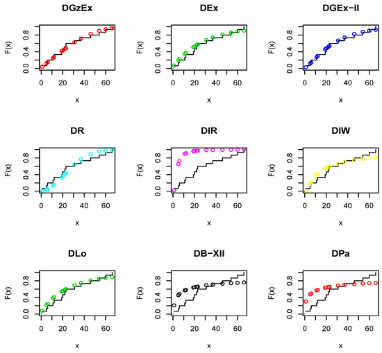
Figure 15. The estimated cumulative distribution functions (CDFs) for Dataset 2.

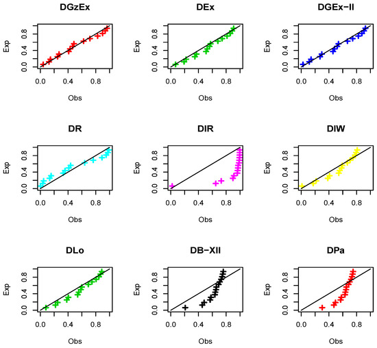
Figure 16. The P-P plots for Dataset 2.

It is clear that the dataset plausibly came from the the DEx, DGEx-II, DR, DIW, and DLo models. However, the the DGzEx model is the best. Table 12 lists some statistics for Dataset 2 using the DGzEx parameters.

Table 12. Some statistics for Dataset 2.

Model	Mean	Var	DsI	Sk	Ku
DGzEx	$27.160$	$358.925$	$13.215$	$0.652$	$2.846$

Regarding Table 12, it is clear that these data suffer from over-dispersion phenomena. Moreover, these data are moderately skewed to the right with platykurtic. The MTTF of these data equals $27.160$whereas the entropy equals $4.354$. Table 13 lists some numerical values of the reliability properties using Dataset 2.

Table 13. Some reliability measures using Dataset 2.

Time $\downarrow$Measure →	RF	HRF	MTBF
2	$0.9584$	$0.0088$	$47.0360$
4	$0.9166$	$0.0092$	$45.9576$
6	$0.8749$	$0.0096$	$44.8959$
8	$0.8332$	$0.1001$	$43.8512$
10	$0.7917$	$0.0105$	$42.8233$
12	$0.7505$	$0.0110$	$41.812$
14	$0.7096$	$0.0115$	$40.8178$
16	$0.6692$	$0.0121$	$39.8401$
18	$0.6294$	$0.0126$	$38.8790$
20	$0.5902$	$0.0132$	$37.9346$
22	$0.5518$	$0.0138$	$37.0067$
24	$0.5143$	$0.0144$	$36.0950$
26	$0.4777$	$0.0151$	$35.2001$
28	$0.4423$	$0.0158$	$34.3212$
30	$0.4079$	$0.0165$	$33.4586$

Regarding Table 13, it is clear that the RF and MTBF decrease, whereas the HRF increases with $t\to \infty$.

7.3. Dataset 3

These data represent the counts of cysts of kidneys using steroids. This dataset originated from a study Chan et al. [49]. For this dataset, we compare the fits of the DGzW distribution with some competitive models such as DW, DIW, DR, DEx, discrete Lindley (DLi), discrete Lindley type II DLi-II, DLo, and Poisson (Poi). The MLEs with their corresponding Std-er, and the goodness of fit statistics are reported in Table 14 and Table 15, respectively.

Table 14. The MLEs with their corresponding Std-er for Dataset 3.

Model ↓ Parameter →	p		c		a		b
	MLE	Std-er	MLE	Std-er	MLE	Std-er	MLE	Std-er
DGzW	$0.490$	$0.073$	$1.630$	$0.021$	$0.670$	$0.690$	$0.320$	$0.290$
DW	−	−	−	−	$0.750$	$0.084$	$0.431$	$0.340$
DIW	−	−	−	−	$0.581$	$0.048$	$1.049$	$0.146$
DR	−	−	−	−	$0.901$	$0.009$	−	−
DEx	−	−	−	−	$0.581$	$0.030$	−	−
DLi	−	−	−	−	$0.436$	$0.026$	−	−
DLi-II	−	−	−	−	$0.581$	$0.045$	$0.001$	$0.058$
DLo	−	−	−	−	$0.150$	$0.098$	$1.830$	$0.951$
Poi	−	−	−	−	$1.390$	$0.112$	−	−

Table 15. The goodness of fit statistics for Dataset 3.

Z	Observed Frequency	Expected Frequency
		DGzW	DW	DIW	DR	DEx	DLi	DLi-II	DLo	Poi
0	65	$64.24$	$59.01$	$63.91$	$11.00$	$46.09$	$40.25$	$46.03$	$61.89$	$27.42$
1	14	$15.44$	$19.84$	$20.70$	$26.83$	$26.78$	$29.83$	$26.77$	$21.01$	$38.08$
2	10	$9.18$	$10.78$	$8.05$	$29.55$	$15.56$	$18.36$	$15.57$	$9.65$	$26.47$
3	6	$6.07$	$6.26$	$4.23$	$22.23$	$9.04$	$10.35$	$9.05$	$5.24$	$12.26$
4	4	$4.20$	$4.19$	$2.60$	$12.49$	$5.25$	$5.53$	$5.27$	$3.17$	$4.26$
5	2	$2.98$	$2.01$	$1.75$	$5.42$	$3.05$	$2.86$	$3.06$	$2.06$	$1.18$
6	2	$2.15$	$1.99$	$1.26$	$1.85$	$1.77$	$1.44$	$1.78$	$1.42$	$0.27$
7	2	$1.56$	$1.32$	$0.95$	$0.52$	$1.03$	$0.71$	$1.04$	$1.02$	$0.05$
8	1	$1.14$	$0.99$	$0.74$	$0.11$	$0.60$	$0.35$	$0.60$	$0.76$	$0.01$
9	1	$0.83$	$0.86$	$0.59$	$0.02$	$0.35$	$0.17$	$0.35$	$0.58$	$0.00$
10	1	$0.61$	$0.76$	$0.48$	$0.00$	$0.20$	$0.08$	$0.20$	$0.46$	$0.00$
11	2	$1.60$	$1.99$	$4.74$	$0.00$	$0.28$	$0.07$	$0.28$	$2.74$	$0.00$
Total	110	110	110	110	110	110	110	110	110	110
$-\mathit{L}$		$167.02$	$170.14$	$172.93$	$277.78$	$178.77$	$189.1$	$178.8$	$170.48$	$246.21$
AIC		$342.05$	$344.28$	$349.87$	$557.56$	$359.53$	$380.2$	$361.5$	$344.96$	$494.42$
CAIC		$342.43$	$344.39$	$349.98$	$557.59$	$359.57$	$380.3$	$361.6$	$345.07$	$494.46$
${\chi }^2$		$0.567$	$3.125$	$6.463$	$321.07$	$22.88$	$43.48$	$22.89$	$3.316$	$294.10$
d.f		1	3	3	4	4	4	3	3	4
p-value		$0.451$	$0.373$	$0.091$	<0.0001	$0.0001$	<0.0001	<0.0001	$0.345$	<0.0001

Regarding Table 15, it is clear that, the DW, DIW, and DLo models work quite well for analyzing these data aside from the DGzW model. However, the the DGzW provides the best fit among all the tested models. Figure 17 and Figure 18 support the results of Table 15.

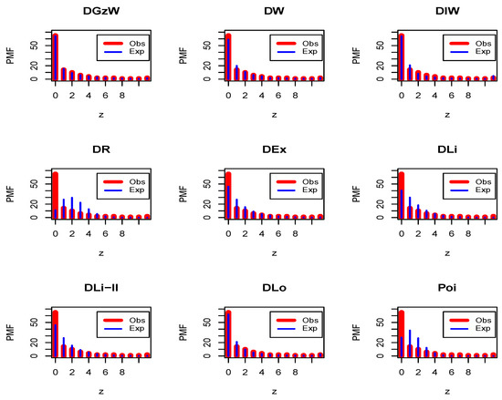
Figure 17. The fitted PMFs for Dataset 3.

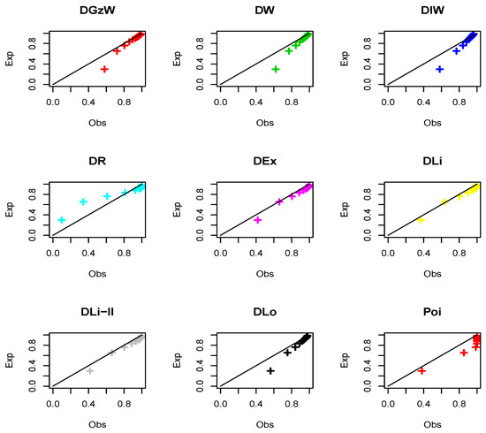
Figure 18. The P-P plots for Dataset 3.

It is clear that the dataset plausibly came from the DGzW, DW, DIW, and DLo models. However, the DGzW model is the best. Table 16 reports some statistics for Dataset 3 based on the DGzW parameters.

Table 16. Some statistics for Dataset 3.

Model	Mean	Var	DsI	Sk	Ku
DGzW	$1.4669$	$7.1318$	$4.8616$	$2.8977$	$14.3679$

According Table 16, it is observed that these data suffer from over-dispersion phenomena. Moreover, these data are moderately skewed to the right with leptokurtic.

7.4. Dataset 4

This dataset is the biological experiment data which represents the number of European corn-borer larvae pyrausta in the field (see Bodhisuwan and Sangpoom [50]). It was an experiment conducted randomly on eight hills in 15 replications, where the experimenter counted the number of borers per hill of corn. We shall compare the fits of the DGzIW distribution with some competitive models such as DIW, DB-XII, DIR, DR, negative binomial (NvBi), DPa, and Poi distributions. The MLEs with their corresponding Std-er as well as goodness of fit statistics for Dataset 4 are listed in Table 17 and Table 18, respectively.

Table 17. The MLEs with their corresponding Std-er for Dataset 4.

Model ↓ Parameter →	p		c		a		b
	MLE	Std-er	MLE	Std-er	MLE	Std-er	MLE	Std-er
DGzIW	$0.0450$	$0.429$	$2.539$	$4.703$	$2.159$	$2.698$	$0.479$	$0.466$
DIW	$0.345$	$0.043$	$1.541$	$0.156$	−	−	−	−
DB-XII	$0.519$	$0.051$	$2.358$	$0.366$	−	−	−	−
DIR	$0.319$	$0.042$	−	−	−	−	−	−
DR	$0.867$	$0.012$	−	−	−	−	−	−
NvBi	$0.870$	$0.036$	$9.956$	$0.096$	−	−	−	−
DPa	$0.329$	$0.034$	−	−	−	−	−	−
Poi	$1.483$	$0.025$	−	−	−	−	−	−

Table 18. The goodness of fit statistics for Dataset 4.

X	Observed Frequency	Expected Frequency
		DGzIW	DIW	DB-XII	DIR	DR	NvBi	DPa	Poi
0	43	$43.20$	$41.37$	$43.84$	$38.28$	$15.92$	$30.12$	$64.45$	$27.23$
1	35	$33.43$	$41.85$	$39.61$	$51.90$	$36.17$	$38.87$	$20.15$	$40.38$
2	17	$18.71$	$15.42$	$15.62$	$15.51$	$34.58$	$27.61$	$9.69$	$29.95$
3	11	$10.56$	$7.17$	$7.20$	$6.04$	$21.03$	$14.26$	$5.65$	$14.81$
4	5	$6.01$	$3.94$	$3.91$	$2.91$	$8.89$	$5.99$	$3.68$	$5.49$
5	4	$3.44$	$2.42$	$2.37$	$1.61$	$2.70$	$2.17$	$2.58$	$1.63$
6	1	$1.98$	$1.61$	$1.56$	$0.98$	$0.60$	$0.70$	$1.90$	$0.40$
7	2	$1.14$	$1.13$	$1.09$	$0.64$	$0.09$	$0.21$	$1.46$	$0.09$
8	2	$1.53$	$5.09$	$4.80$	$2.14$	$0.02$	$0.06$	$10.44$	$0.02$
Total	120	120	120	120	120	120	120	120	120
$-\mathit{L}$		$200.018$	$204.810$	$204.293$	$208.440$	$235.23$	$211.52$	$220.63$	$219.19$
AIC		$408.035$	$413.621$	$412.587$	$418.881$	$472.45$	$427.05$	$443.24$	$440.38$
CAIC		$408.383$	$413.723$	$412.689$	$418.915$	$472.49$	$427.14$	$443.27$	$440.41$
${\chi }^2$		$0.521$	$5.511$	$4.664$	$14.274$	$70.688$	$20.367$	$32.462$	$38.478$
d.f		1	3	3	4	4	3	4	4
P.value		$0.470$	$0.138$	$0.198$	$<0.0001$	$<0.0001$	$0.0001$	$<0.0001$	$<0.0001$

According to Table 18, it is observed that both the DIW and DB-XII models work quite well aside from the DGzIW model. However, the DGzIW model is the best for these data. Figure 19 and Figure 20 support the results of Table 18.

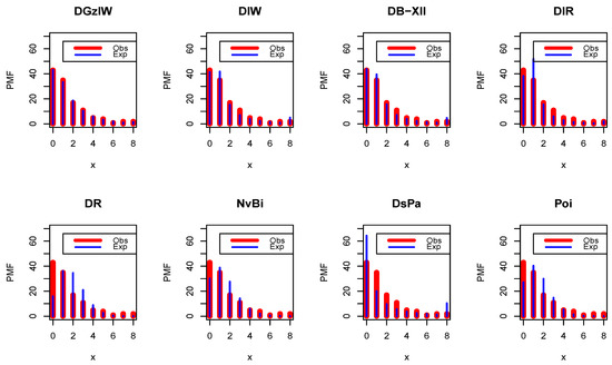
Figure 19. The fitted PMFs for Dataset 4.

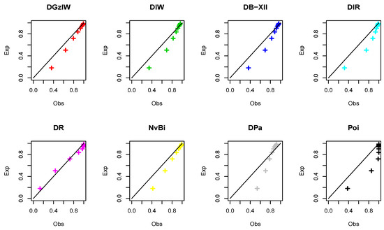
Figure 20. The P-P plots for Dataset 4.

It is clear that the dataset plausibly came from the DGzIW model. Moreover, it is considered the best model among all the tested models. Table 19 lists some statistics for Dataset 4 based on the DGzIW parameters.

Table 19. Some statistics for Dataset 4.

Model	Mean	Var	DsI	Sk	Ku
DGzIW	$1.632$	$3.641$	$2.231$	$1.900$	$8.312$

Regarding Table 19, it is observed that the data suffers from over-dispersion. Moreover, these data are moderately skewed to the right with leptokurtic.

8. Concluding Remarks

In this article, we propose a new discrete family of distributions, in the so-called DGz-G family. Several of its statistical properties were studied. Three special models of the new family are discussed in detail. It is found that the proposed family is capable of modeling a negatively skewed, a positively skewed, or a symmetric shape, and the HRF can take different shapes. Further, it is appropriate for modeling both over- and under-dispersed data. The proposed family can be used for modeling count and lifetime data. The maximum likelihood method was used for estimating the family parameters. A simulation study was carried out to assess the performance of the family parameters. It is found that the maximum likelihood method performs quite well in estimating the model parameters. Finally, the flexibility of the proposed family was illustrated by means of four distinctive datasets. The aim of the present work is to attract wider applications in medicine, engineering, and other fields of research.

References

- Willemse, W.J.; Koppelaar, H. Knowledge elicitation of Gompertz’s law of mortality. Scand. Actuar. J. 2000, 2, 168–179. [Google Scholar] [CrossRef]
- Preston, S.H.; Heuveline, P.; Guillot, M. Demography: Measuring and Modeling Population Processes; Blackwell: Oxford, UK, 2001. [Google Scholar]
- Melnikov, A.; Romaniuk, Y. Evaluating the performance of Gompertz, Makeham and Lee-Carter mortality models for risk management with unit-linked contracts. Insur. Math. Econ. 2006, 39, 310–329. [Google Scholar] [CrossRef]
- Ohishi, K.; Okamura, H.; Dohi, T. Gompertz software reliability model: Estimation algorithm and empirical validation. J. Syst. Softw. 2009, 82, 535–543. [Google Scholar] [CrossRef]
- Bemmaor, A.C.; Glady, N. Modeling Purchasing Behavior With Sudden ‘Death’: A Flexible Customer Lifetime Model. Manag. Sci. 2012, 58, 1012–1021. [Google Scholar] [CrossRef]
- Cordeiro, G.M.; Alizadeh, M.; Abraao, D.C.; Mahdi, R. The exponentiated Gompertz generated family of distributions: Properties and applications. Chil. J. Stat. 2016, 7, 29–50. [Google Scholar]
- El-Bassiouny, A.H.; Medhat, E.L.; Mustafa, A.; Eliwa, M.S. Characterization of the Generalized Weibull-Gompertz Distribution Based on the Upper Record Values. Int. J. Math. Appl. 2015, 3, 13–22. [Google Scholar]
- El-Bassiouny, A.H.; EL-Damcese, M.; Mustafa, A.; Eliwa, M.S. Exponentiated generalized Weibull-Gompertz distribution with application in survival analysis. J. Stat. Appl. Probab. 2017, 6, 7–16. [Google Scholar] [CrossRef]
- El-Bassiouny, A.H.; EL-Damcese, M.; Mustafa, A.; Eliwa, M.S. Mixture of exponentiated generalized Weibull-Gompertz distribution and its applications in reliability. J. Stat. Appl. Probab. 2016, 5, 1–14. [Google Scholar] [CrossRef]
- Alzaatreh, A.; Lee, C.; Famoye, F. A new method for generating families of continuous distributions. Metron 2013, 71, 63–79. [Google Scholar] [CrossRef]
- Roozegar, R.; Tahmasebi, S.; Jafari, A.A. The McDonald Gompertz distribution: Properties and applications. Commun. Stat.-Simul. Comput. 2017, 46, 3341–3355. [Google Scholar] [CrossRef]
- Mazucheli, J.; Menezes, A.F.; Dey, S. Unit-Gompertz distribution with applications. Statistica 2019, 79, 25–43. [Google Scholar]
- Eliwa, M.S.; El-Morshedy, M.; Ibrahim, M. Inverse Gompertz distribution: Properties and different estimation methods with application to complete and censored data. Ann. Data Sci. 2019, 6, 321–339. [Google Scholar] [CrossRef]
- Alizadeh, M.; Cordeiro, G.M.; Luis, G.B.; Indranil, G. The Gompertz-G family of distributions. J. Stat. Theory Pract. 2017, 11, 179–207. [Google Scholar] [CrossRef]
- El-Morshedy, M.; Eliwa, M.S. The odd flexible Weibull-H family of distributions: Properties and estimation with applications to complete and upper record data. Filomat 2019, 33, 2635–2652. [Google Scholar] [CrossRef]
- Eliwa, M.S.; El-Morshedy, M. Bivariate Gumbel-G family of distributions: Statistical properties, Bayesian and non-Bayesian estimation with application. Ann. Data Sci. 2019, 6, 39–60. [Google Scholar] [CrossRef]
- Eliwa, M.S.; El-Morshedy, M. Bivariate odd Weibull-G family of distributions: Properties, Bayesian and non-Bayesian estimation with bootstrap confidence intervals and application. J. Taibah Univ. Sci. 2020, 14, 1–22. [Google Scholar]
- Alizadeh, M.; Afify, A.Z.; Eliwa, M.S.; Ali, S. The odd log-logistic Lindley-G family of distributions: Properties, Bayesian and non-Bayesian estimation with applications. Comput. Stat. 2020, 35, 281–308. [Google Scholar] [CrossRef]
- Eliwa, M.S.; Alhussain, Z.A.; Ahmed, E.A.; Salah, M.M.; Ahmed, H.H.; El-Morshedy, M. Bivariate Gompertz generator of distributions: Statistical properties and estimation with application to model football data. J. Natl. Sci. Found. Sri Lanka 2020, 48, 54–72. [Google Scholar]
- Eliwa, M.S.; El-Morshedy, M.; Afify, A.Z. The odd Chen generator of distributions: Properties and estimation methods with applications in medicine and engineering. J. Natl. Sci. Found. Sri Lanka 2020, 48, 1–23. [Google Scholar]
- El-Morshedy, M.; Alhussain, Z.A.; Atta, D.; Almetwally, E.M.; Eliwa, M.S. Bivariate Burr X generator of distributions: Properties and estimation methods with applications to complete and type-II censored samples. Mathematics 2020, 8, 264. [Google Scholar] [CrossRef]
- Roy, D. Discrete Rayleigh distribution. IEEE Trans. Reliab. 2004, 53, 255–260. [Google Scholar] [CrossRef]
- Gómez-Déniz, E. Another generalization of the geometric distribution. Test 2010, 19, 399–415. [Google Scholar] [CrossRef]
- Bebbington, M.; Lai, C.D.; Wellington, M.; Zitikis, R. The discrete additive Weibull distribution: A bathtub-shaped hazard for discontinuous failure data. Reliab. Eng. Syst. Saf. 2012, 106, 37–44. [Google Scholar] [CrossRef]
- Nooghabi, M.S.; Borzadaran, G.R.; Roknabadi, A.H. Discrete modified Weibull distribution. Metron 2012, 69, 207–222. [Google Scholar] [CrossRef]
- Nekoukhou, V.; Alamatsaz, M.H.; Bidram, H. Discrete generalized exponential distribution of a second type. Statistics 2013, 47, 876–887. [Google Scholar] [CrossRef]
- Bakouch, H.S.; Aghababaei, M.; Nadarajah, S. A new discrete distribution. Statistics 2014, 48, 200–240. [Google Scholar] [CrossRef]
- Nekoukhou, V.; Bidram, H. The exponentiated discrete Weibull distribution. Stat. Oper. Res. Trans. 2015, 39, 127–146. [Google Scholar]
- Chandrakant, K.; Yogesh, M.T.; Manoj, K.R. On a discrete analogue of linear failure rate distribution. Am. J. Math. Manag. Sci. 2017, 36, 229–246. [Google Scholar]
- Para, B.A.; Jan, T.R. Discrete inverse Weibull minimax distribution. J. Stat. Appl. Probab. 2017, 6, 205–218. [Google Scholar] [CrossRef]
- Mazucheli, J.; Bertoli, W.; Oliveira, R.P. On the discrete quasi Xgamma distribution. Methodol. Comput. Appl. Probab. 2019. [Google Scholar] [CrossRef]
- El-Morshedy, M.; Eliwa, M.S.; El-Gohary, A.; Khalil, A.A. Bivariate exponentiated discrete Weibull distribution: Statistical properties, estimation, simulation and applications. Math. Sci. 2019, 1–14. [Google Scholar] [CrossRef]
- Eliwa, M.S.; El-Morshedy, M. A one-parameter discrete distribution for over-dispersed data: Statistical and reliability properties with estimation approaches and applications. J. Appl. Stat. 2020, 47, 184–205. [Google Scholar]
- Rényi, A. On measures of entropy and information. Math. Stat. Probab. 1961, 1, 547–561. [Google Scholar]
- Hosking, J.R.; Wallis, J.R. Regional Frequency Analysis: An Approach Based on L-Moments; Cambridge University Press: Cambridge, UK, 1997. [Google Scholar]
- Kundu, D.; Nekoukhou, V. Univariate and bivariate geometric discrete generalized exponential distributions. J. Stat. Theory Pract. 2018, 12, 595–614. [Google Scholar] [CrossRef]
- Nakagawa, T.; Osaki, S. The discrete Weibull distribution. IEEE Trans. Reliab. 1975, 24, 300–301. [Google Scholar] [CrossRef]
- Jazi, A.M.; Lai, D.C.; Alamatsaz, H.M. Inverse Weibull distribution and estimation of its parameters. Stat. Methodol. 2010, 7, 121–132. [Google Scholar] [CrossRef]
- Hussain, T.; Ahmad, M. Discrete inverse Rayleigh distribution. Pak. J. Stat. 2014, 30, 203–222. [Google Scholar]
- Gómez-Déniz, E.; Calderín-Ojeda, E. The discrete Lindley distribution: Properties and applications. J. Stat. Comput. Simul. 2011, 81, 1405–1416. [Google Scholar] [CrossRef]
- El-Morshedy, M.; Eliwa, M.S.; Nagy, H. A new two-parameter exponentiated discrete Lindley distribution: Properties, estimation and applications. J. Appl. Stat. 2020, 47, 354–375. [Google Scholar] [CrossRef]
- Hussain, T.; Aslam, M.; Ahmad, M. A Two parameter discrete Lindley distribution. Rev. Colomb. Estadística 2016, 39, 45–61. [Google Scholar] [CrossRef]
- Para, B.A.; Jan, T.R. Discrete version of log-logistic distribution and its applications in genetics. Int. J. Mod. Math. Sci. 2016, 14, 407–422. [Google Scholar]
- Para, B.A.; Jan, T.R. On discrete three-parameter Burr type XII and discrete Lomax distributions and their applications to model count data from medical science. Biom. Biostat. Int. J. 2016, 4, 1–15. [Google Scholar]
- Krishna, H.; Pundir, P.S. Discrete Burr and discrete Pareto distributions. Stat. Methodol. 2009, 6, 177–188. [Google Scholar] [CrossRef]
- Dougherty, E.R. Probability and Statistics for the Engineering, Computing and Physical Sciences; Prentice Hall: Englewood Cliffs, NJ, USA, 1992; pp. 149–152. ISBN 0-13-711995-X. [Google Scholar]
- Poisson, S.D. Probabilité des Jugements en Matiére Criminelle et en Matiére Civile, Précédées des RéGles Génerales du Calcul des Probabilitiés; Bachelier: Paris, France, 1837; pp. 206–207. [Google Scholar]
- Lawless, J.F. Statistical Models and Methods for Lifetime Data; Wiley: New York, NY, USA, 2003. [Google Scholar]
- Chan, S.; Riley, P.R.; Price, K.L.; McElduff, F.; Winyard, P.J. Corticosteroid-induced kidney dysmorphogenesis is associated with deregulated expression of known cystogenic molecules, as well as Indian hedgehog. Am. J. Physiol.-Ren. Physiol. 2009, 298, 346–356. [Google Scholar] [CrossRef]
- Bodhisuwan, W.; Sangpoom, S. The discrete weighted Lindley distribution. In Proceedings of the International Conference on Mathematics, Statistics, and Their Applications, Banda Aceh, Indonesia, 4–6 October 2016. [Google Scholar]
© 2020 by the authors. Licensee MDPI, Basel, Switzerland. This article is an open access article distributed under the terms and conditions of the Creative Commons Attribution (CC BY) license (http://creativecommons.org/licenses/by/4.0/).