A Discontinuous ODE Model of the Glacial Cycles with Diffusive Heat Transport

Abstract

We present a new discontinuous ordinary differential equation (ODE) model of the glacial cycles. Model trajectories flip from a glacial to an interglacial state, and vice versa, via a switching mechanism motivated by ice sheet mass balance principles. Filippov’s theory of differential inclusions is used to analyze the system, which can be viewed as a nonsmooth geometric singular perturbation problem. We prove the existence of a unique limit cycle, corresponding to the Earth’s glacial cycles. The diffusive heat transport component of the model is ideally suited for investigating the competing temperature gradient and transport efficiency feedbacks, each associated with ice-albedo feedback. It is the interplay of these feedbacks that determines the maximal extent of the ice sheet. In the nonautonomous setting, model glacial cycles persist when subjected to external forcing brought on by changes in Earth’s orbital parameters over geologic time. The system also exhibits various bifurcation scenarios as key parameters vary.

1. Introduction

Earth’s climate has varied drastically over long time scales, cycling between warmer interglacial periods and very cold glacial states (ice ages). The beginning of a glacial cycle is characterized by a slow descent into a much colder world, in which massive ice sheets advanced into North America and Eurasia, fed by the moisture resulting from a corresponding drop in sea level of about 350 feet [1]. The ice ages are followed by a relatively rapid retreat into interglacial periods, leading to a sawtooth pattern evident in the paleoclimate data (Figure 1).

While large-scale climate models are able to provide insight into glacial cycle dynamics [2], the use of a comprehensive Earth System Model to accurately simulate even the last glacial cycle remains a challenge [3]. As such, approaches such as the analysis of data from deep ocean sediment cores [4] and Greenland and Antarctic ice cores [5], and the use of conceptual (or low order, reduced) climate models, also play important roles in the investigation of climate phenomena associated with glacial cycles [6,7,8,9,10,11,12,13,14,15]. As the time scales of related climate phenomena can differ to a great degree, conceptual models often involve a switching mechanism and nonsmooth model equations [13,16,17,18,19,20]. The model introduced here will contain a climate switching mechanism, leading to an associated nonsmooth geometric singular perturbation problem. We prove the existence of a unique attracting (nonsmooth) limit cycle that corresponds to the glacial-interglacial oscillations.

Numerous questions regarding the glacial cycles remain unanswered, beginning with those related to the frequency and amplitude of the oscillations. Many believe the pacing of the ice ages is related to changes in Earth’s orbital parameters, known as Milankovitch cycles [21]. For example, the obliquity (or tilt) of the Earth’s spin axis has varied over the past 5 million years [22] with a period of about 41 kyr. It is known that, between 3 and 1.2 million years ago, the glacial cycles oscillated with a dominant period of 41 kyr as well [4].

Over the past 800 kyr, ice ages were of longer duration and the period of the glacial cycles grew to about 100 kyr, with the amplitude of the cycles increasing as well (Figure 1). Interestingly, the eccentricity of the Earth’s orbit has varied over geologic time with a period of roughly 100 kyr. Understanding this change to larger amplitude, smaller frequency glacial cycles between 1200 and 800 thousand years ago—known as the Mid-Pleistocene Transition (MPT)—and the nature of the climate response to the external forcing provided by the Milankovitch cycles, continues as a major open problem in paleoclimate. From a dynamical systems perspective, a phenomenon such as the MPT is testament to the complexity of the climate system and the often nonlinear response of the climate system to external forcing.

Additional questions concern internal climate feedbacks and the possibility of self-sustained oscillations, which represent the main focus of this paper. Foremost among these from a conceptual modeling perspective is positive ice-albedo feedback. An expanding ice sheet leads to a higher albedo and reduced absorption of solar radiation, thereby reducing temperature and further enhancing growth of the ice sheet. Similarly, a retreating ice sheet leads to an increase in absorption of solar radiation and higher temperatures, contributing to further ice sheet loss.

The role of ice-albedo feedback as it relates to zonally averaged (by latitude) surface temperature was studied in the seminal work of Budyko [7] and Sellers [14] in 1969. Budyko’s surface temperature model was coupled with an ODE for the evolution of the edge of the ice sheet (known as the ice line) in [15], where it was shown the ice line either converges to a small stable ice cap equilibrium position or descends to the equator (with parameters aligned with the modern climate). The latter outcome is known as a runaway snowball Earth episode.

The potential for self-sustained climate oscillations might arise via consideration of competing feedbacks associated with ice-albedo feedback [8,9]. For example, at the onset of a glacial age, a descending ice sheet leads to an increase in the surface temperature gradient, due to the increased albedo in the polar region. This leads to a positive feedback in that the poleward transport of heat and moisture by the atmosphere, with the moisture precipitating out as snow on the glacier, is enhanced, all things being equal [23]. In this way, the ice sheet continues to grow.

A competing, negative feedback is that the efficiency of the meridional heat and moisture transport is decreased as the ice sheet advances. In the conceptual model setting, North [24] proposed that the efficiency of the meridional transport might have two values, the smaller of which corresponds to the portion of the planet covered by ice. That is, a planet with extensive ice cover will be less efficient in the transport of heat and moisture poleward (also see [25]). The thinking is that an increase in sea ice during a glacial advance serves to reduce heat advection in the oceans. Due to atmospheric-oceanic coupling, together with extensive sea ice, evaporation and the transport of moisture will each be impaired.

Similarly, as albedo decreases during a glacial retreat, the meridional temperature gradient weakens, impacting the poleward transport of moisture. However, the efficiency of the meridional transport might be assumed to increase as the sea ice retreats, with ocean advection and the coupling between the atmosphere and the ocean enhanced. Thus, the efficiency of the diffusive transport across latitudes can be viewed as a negative feedback with respect to ice sheet growth.

We investigate the interaction between this negative feedback and the positive temperature gradient feedback described above in the conceptual model, ODE setting. We do this in part by assuming the diffusive meridional transport efficiency parameter is smaller during a glacial advance, relative to that during a glacial retreat, due to the ice cover.

2. Results

We present a new conceptual model of the glacial cycles in which the latitudinal transport of heat is modeled as a diffusive process. The zonal surface temperature PDE is coupled to the ice line, as in [15]. The spectral method is used to approximate the resulting infinite dimensional system with a finite system of ODEs. Standard invariant manifold theory [26] is used to reduce this finite system to a single governing equation on a slow manifold, corresponding to the evolution of the edge of the ice sheet.

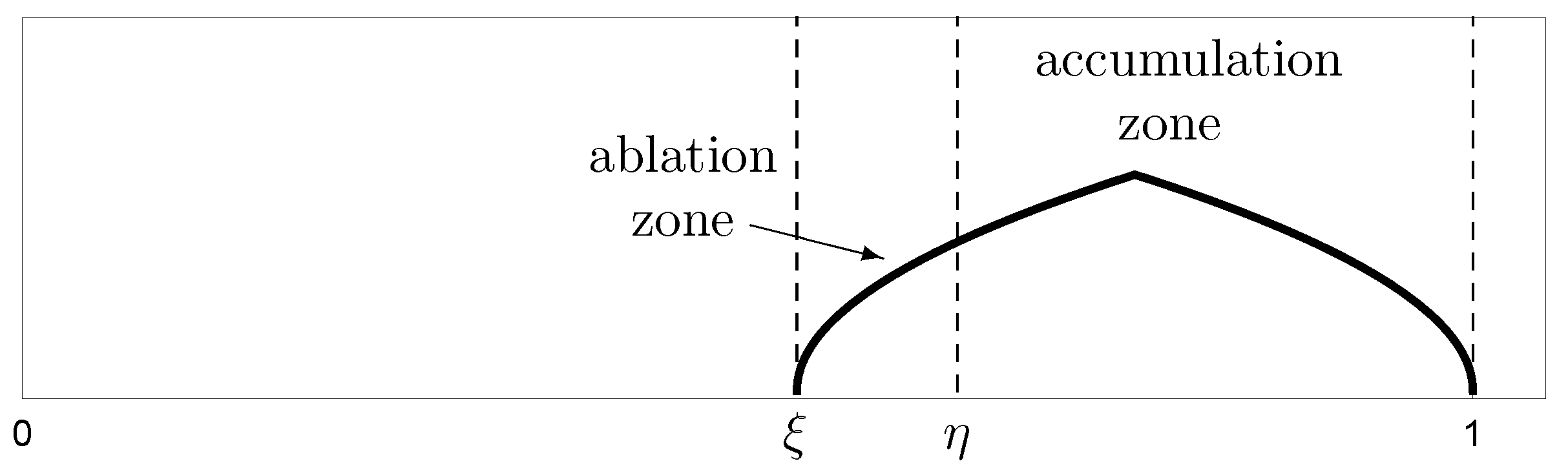
Consideration of ablation and accumulation zones on the ice sheet leads to the introduction of a second model variable, as in [20]. The incorporation of a switching mechanism based on an ice sheet mass balance equation into this two-dimensional system, as described below, leads to a differential inclusion. Using Filippov’s approach to differential inclusions [27], a unique attracting (nonsmooth) limit cycle is shown to exist, with the Contraction Mapping Theorem the major tool used in the proof. This periodic orbit, a consequence of the competing feedbacks discussed in the Introduction, represents internal, self-sustained climate oscillations.

Similar in spirit to Welander’s mixed ocean layer heat-salt oscillator [28], two virtual equilibria play a fundamental role in the limit cycle produced here. Varying a model parameter leads to a type of nonsmooth Hopf bifurcation, arising as a border collision bifurcation, as is discussed along with additional bifurcation scenarios in the following.

It is of interest to note that forcing our model with variations in eccentricity and obliquity does not significantly affect the glacial-interglacial oscillations in a qualitative sense. The dynamics of this nonautonomous, nonsmooth model are presented below.

This paper is organized as follows. The model equations are derived in Section 3. The switching mechanism and the set up of the Filippov flow are presented in Section 4. The nonsmooth model flow is analyzed in Section 5, in which the existence of a unique attracting limit cycle is proved. We revisit, and place within the context of the model, the competing feedbacks discussed above by considering the flux at the albedo line throughout the glacial cycle in Section 6. We discuss bifurcations exhibited by the model in Section 7, while the effect of forcing the model with Milankovitch cycles is presented in Section 8. The concluding section contains comments pertaining to open questions, both of a mathematical nature and as they relate to Earth’s glacial cycles, that might be investigated in a conceptual fashion with our model.

3. Model Equations

3.1. The Zonal Average Surface Temperature Equation

The model development begins with the equation for the annual average surface temperature $T=T(y,t){(}^{\circ }$C) at $y=sin\theta$, where $\theta$ denotes latitude. Hence, T is a zonal average, with a single spatial variable y. Due to an assumption of symmetry of the temperature distribution about the equator as in [7], one takes $y\in [0,1]$. Note that $y=0$ and $y=1$ correspond to the equator and North Pole, respectively.

The equation

$$R\frac{\partial T}{\partial t}=Qs\left(y\right)(1-\alpha (y,\eta ))-(A+BT)+D\frac{\partial }{\partial y}(1-y^2)\frac{\partial T}{\partial y},$$

(1)

of a type first introduced by Budyko [7] and Sellers [14], is derived from energy balance principles. The behavior of equilibrium solutions of Equation (1) in response to changes in a given parameter was well studied by North and colleagues in the 1970s and early 1980s [24,29,30,31].

The units on each side of (1) are watts per square meter (W/m${}^2$). The constant R, with units joules per square meter per degree Celsius, denotes the global average heat capacity of the Earth’s surface; the value $R=0.5\times {10}^9$ J/(m${}^2{}^{\circ }$C) used here lies within the range of estimates provided in [32].

Q (W/m${}^2$) is the global average annual incoming solar radiation (or insolation). While $Q=Q\left(e\right)$ depends upon the eccentricity e of the Earth’s orbit over long time scales [11], varying between roughly 342.95 and 343.52 over the past 5 million years [22], we set $Q=343$ W/m${}^2$ in this section.

The function

$$s\left(y\right)=\frac{2}{{\pi }^2}{\int }_0^{2\pi }\sqrt{1-{(\sqrt{1-y^2}sin\beta cos\gamma -ycos\beta )}^2}d\gamma$$

(2)

is the insolation distribution function [11], accounting for the fact that, on Earth, tropical latitudes receive greater annual mean insolation than do polar regions. The function $s\left(y\right)$ satisfies the normalizing condition

$${\int }_0^{1}s\left(y\right)dy=1.$$

In addition, $s\left(y\right)$ depends on the obliquity $\beta$ of the Earth’s spin axis. The obliquity has varied between roughly 22${}^{\circ }$ and 24.5${}^{\circ }$ over geologic time, with the current value of $\beta$ approximately equal to 23.4${}^{\circ }$.

The function

$$\alpha (y,\eta )=\left\{\begin{array}{cc}{\alpha }_1,\hfill & \mathrm{if}y<\eta \hfill \\ {\alpha }_2,\hfill & \mathrm{if}y>\eta ,\hfill \end{array}\right.$$

(3)

where ${\alpha }_1<{\alpha }_2,$ represents the reflectivity or albedo of the Earth’s surface. The ice line is denoted by $\eta$; following Budyko in [7], one assumes $\eta$ separates latitudes of high albedo ${\alpha }_2$ poleward of $\eta$ from latitudes of lower albedo ${\alpha }_1$ equatorward of $\eta$. Taken together, the expression $Qs\left(y\right)(1-\alpha (y,\eta \left)\right)$ in (1) models the energy into the climate system.

The $(A+BT)$-term represents the outgoing longwave radiation (OLR), or energy out of the climate system. The parameters $A>0$ (W/m${}^2$) and $B>0$ (W/(m${}^2$${}^{\circ }$C) have been estimated empirically [33] (see

Table 1. Parameter values.

Parameter	Value	Units	Parameter	Value	Units
Q	343	Wm${}^{-2}$	$T_c$	$-10$	${}^{\circ }$C
A	202	Wm${}^{-2}$	$b_G$	1.5	dimensionless
B	1.9	Wm${}^{-2}{{(}^{\circ }\mathrm{C})}^{-1}$	b	1.75	dimensionless
$D_G$	0.3	Wm${}^{-2}{{(}^{\circ }\mathrm{C})}^{-1}$	$b_I$	4	dimensionless
$D_I$	0.394	Wm${}^{-2}{{(}^{\circ }\mathrm{C})}^{-1}$	a	1.05	dimensionless
${\alpha }_1$	0.32	dimensionless	R	$0.5\times {10}^9$	J/(m${}^2{}^{\circ }$C)
${\alpha }_2$	0.62	dimensionless	$\beta$	23.4${}^{\circ }$

). That the Earth’s OLR is essentially linear over a wide range of surface temperature values is presented in [34].

The final term in (1) models the meridional transport of heat by the atmosphere and ocean as a diffusive process, with $D>0$ (W/(m${}^2$ ${}^{\circ }$C) the diffusion coefficient. Recalling $y=sin\theta$ and that $T(y,t)$ has no longitudinal dependence, the spherical diffusion operator takes the form

$$\nabla ·(D\nabla T)=D\frac{\partial }{\partial y}(1-y^2)\frac{\partial T}{\partial y}$$

(4)

(see, for example, [24]). A mean annual temperature model with symmetry about the equator must satisfy boundary conditions, namely, that the gradient of the temperature vanishes at the North Pole and at the equator. That this is the case in our approach is shown in Section 3.2.

While Budyko modeled meridional heat transport in [7] via the expression

$$C(T_{\mathrm{ave}}-T),$$

(5)

where $C>0$ and $T_{\mathrm{ave}}$ is the annual global mean surface temperature, Equation (4) has the advantage that the Legendre polynomials $P_n\left(y\right)$ are eigenfunctions of the spherical diffusion operator

$$\frac{d}{dy}(1-y^2)\frac{d}{dy}{P}_n\left(y\right)=-n(n+1)P_n\left(y\right),n=0,1,2,\dots$$

(6)

We make use of this observation in the following section.

3.2. The Spectral Approach

We approximate Equation (1) via a finite system of ODEs by taking advantage of (6).

For a fixed ice line $\eta$, this is the approach used by North in works such as [24,29]. (In the following section, the ice line will be allowed to evolve over time, coupled to the temperature equation as in [15].) Full details of the following derivation can be found in [35]. We assume the obliquity $\beta ={23.4}^{\circ }$ in the following.

Recall $T(y,t)$ is an even function of y, given the assumed symmetry of the temperature profile about $y=0$. Let $P_{2i},i=0,\dots ,N$, denote the first $N+1$ even Legendre polynomials. Write

$$T(y,t)=\sum _{i=0}^N{T}_{2i}\left(t\right)P_{2i}\left(y\right).$$

(7)

Note the even Legendre polynomials satisfy

$$\frac{d{P}_{2n}}{d\theta }=\frac{d{P}_{2n}}{dy}cos\theta =0$$

at the equator ($y=0$) and North Pole ($\theta =\frac{\pi }{2}$). Hence, expression (7) satisfies the prescribed boundary conditions.

Similarly, express

$$s\left(y\right)=\sum _{i=0}^N{s}_{2i}{P}_{2i}\left(y\right)$$

(8)

and

$$\alpha (y,\eta )s\left(y\right)=\sum _{i=0}^N{\overline{\alpha }}_{2i}\left(\eta \right)P_{2i}\left(y\right)$$

(9)

where, for $i=0,\dots ,N,$

$$s_{2i}=(4i+1){\int }_0^{1}s\left(y\right)P_{2i}\left(y\right)dy$$

(10)

and

$$\begin{array}{cc}\hfill {\overline{\alpha }}_{2i}\left(\eta \right)& =(4i+1){\int }_0^1\alpha (y,\eta )s\left(y\right)P_{2i}\left(y\right)dy\hfill \\ \hfill & ={\alpha }_2{s}_{2i}-(4i+1)({\alpha }_2-{\alpha }_1){\int }_0^{\eta }s\left(y\right)P_{2i}\left(y\right)dy.\hfill \end{array}$$

(11)

Nadeau and McGehee provide a mechanism for the computation of the coefficients $s_{2i}$ (as functions of the obliquity $\beta$) in [36]. We also note the dependence of ${\overline{\alpha }}_{2i}$ on the ice line $\eta$, arising from the substitution of albedo function (3) into the integrand in (11). In particular, ${\overline{\alpha }}_{2i}$ is a polynomial in $\eta$ of degree $4N+1$.

Substituting (7)–(9) into PDE (1) and equating coefficients of $P_{2i}$, one arrives at a system of $N+1$ ODEs that can be placed in the form

$$\frac{d{T}_{2i}}{dt}=-\frac{(B+2i(2i+1\left)D\right)}{R}(T_{2i}-f_{2i}\left(\eta \right)),i=0,\dots ,N,$$

(12)

where

$$\begin{array}{cc}\hfill f_0\left(\eta \right)& =\frac{1}{B}(Q(s_0-{\overline{\alpha }}_0\left(\eta \right))-A),\hfill \\ \hfill \\ \hfill f_{2i}\left(\eta \right)& =\frac{Q}{(B+2i(2i+1\left)D\right)}(s_{2i}-{\overline{\alpha }}_{2i}\left(\eta \right)),i=1,\dots ,N.\hfill \end{array}$$

(13)

In this fashion, solutions to the $N+1$ equations in system (12) serve to approximate solutions to Equation (1).

For future reference, note that, for a fixed ice line $\eta ,T_{2i}\left(t\right)\to f_{2i}\left(\eta \right)$ as $t\to \infty$ for each i, leading to a globally attracting curve of rest points and an associated equilibrium temperature distribution

$$T_{\eta }^{\ast }\left(y\right)=\sum _{i=0}^N{f}_{2i}\left(\eta \right)P_{2i}\left(y\right),$$

(14)

each parametrized by $\eta$. E. Widiasih introduced an equation for the evolution of the ice line $\eta$ that was coupled to the zonal average surface temperature in a simple fashion in [15]. This additional equation will aid consideration of the feedbacks discussed in the Introduction. We incorporate this model enhancement in the following section.

3.3. A Dynamic Ice Line

It is natural to allow the ice line to respond to changes in the zonally averaged surface temperature, a concept introduced and formalized in [15]. The equation

$$R\frac{d\eta }{dt}=\rho (T(\eta ,t)-T_c),\rho >0$$

(15)

considers the temperature at the ice line $\eta$, relative to a critical temperature $T_c$. If $T(\eta ,t)>T_c,$$\eta$ increases as the ice line moves poleward, while $\eta$ decreases and the ice line moves equatorward if $T(\eta ,t)<T_c$. Coupling Equation (15) with system (12), and evaluating (7) at $\eta$, leads to the system of $N+2$ ODEs

$$\begin{array}{cc}\hfill \frac{d{T}_{2i}}{dt}& =-\frac{(B+2i(2i+1\left)D\right)}{R}(T_{2i}-f_{2i}\left(\eta \right)),i=0,\dots ,N,\hfill \end{array}$$

(16a)

$$\begin{array}{cc}\hfill \frac{d\eta }{dt}& =\frac{\rho }{R}\left(\sum _{i=0}^N{T}_{2i}{P}_{2i}\left(\eta \right)-T_c\right).\hfill \end{array}$$

(16b)

Note that when $\rho =0$ we return to the fixed ice line case and a globally attracting curve of rest points on which $T_{2i}=f_{2i}\left(\eta \right)$, as described above. Via standard invariant manifold theory [26], this curve of rest points perturbs to a nearby globally attracting invariant manifold, on which system (16) can be approximated by Equation (16b) with $T_{2i}=f_{2i}\left(\eta \right)$, namely

$$\frac{d\eta }{dt}=\frac{\rho }{R}\left(\sum _{i=0}^N{f}_{2i}\left(\eta \right)P_{2i}\left(\eta \right)-T_c\right)=\frac{\rho }{R}h\left(\eta \right).$$

(17)

That is, Equation (17) is a good approximation to the coupled temperature-ice line system (16) if it is assumed that the ice line changes slowly relative to changes in the temperature. Evidence that this latter assumption is reasonable is provided in [12].

Graphs of $h\left(\eta \right)$, a polynomial of degree $4N+3$, are plotted in Figure 2 for various D-values (the use of subscripts G (glacial) and I (interglacial) in Figure 2 is fully explained in Section 4). Note that, for $D=0.3$ and $N=1$, Equation (17) has an unstable equilibrium with the ice line at roughly $\eta =0.2$ corresponding to a very large ice cap, and a stable, small ice cap equilibrium at about $\eta =0.8$ (the blue curves in Figure 2a,b). To each of these equilibrium $\eta$-vales, there is an associated equilibrium temperature profile $T_{\eta }^{\ast }\left(y\right)$ given by Equation (14).

A diffusion coefficient value of $D=0.394$ is required to place the stable equilibrium near $\eta =0.94$ when $N=1$, roughly positioned to match the Earth’s current polar ice cap extent and climate (the red curves in Figure 2a,b). That is, if at equilibrium $\eta =0.94$ when $N=1$, the choice of $D=0.394$ yields a global mean surface temperature of 15 ${}^{\circ }$C, approximately equal to today’s value. We note the existence of an unstable equilibrium $\eta$-value between $\eta =0.94$ and the North Pole when $\eta =0.394$ (Figure 2b). While working solely with equilibrium solutions of temperature Equation (1) and a fixed ice line, and with “stability” considered with respect to changes in the parameter Q rather than with changes in $\eta$ as considered here, North analyzed the existence of this small unstable ice cap in [30]. In particular, North discussed the connection between the use of the diffusive heat transport mechanism (4) and this small unstable ice cap, while also commenting on the lack of such an equilibrium solution when using Budyko’s transport term (5).

We note the stable-unstable small ice cap pair is lost through a saddle node bifurcation as D increases through roughly $D=0.4$ (see Figure 3). Hence, if the meridional heat transport is sufficiently efficient, the climate tends to either an ice-free Earth or a snowball Earth, depending on the initial position of the ice line relative to the large unstable ice cap $\eta$-value. Finally, the use of higher order approximations does not change the qualitative nature of solutions of Equation (17), as illustrated in Figure 2c, for which all expansions were taken out to degree 6.

3.4. Incorporating Accumulation and Ablation Zones

Note the role of $\eta$ as defined in albedo function (3) is more accurately viewed as an “albedo line," or more germanely to our model, as a snow line. At locations above $\eta$, the surface has a higher albedo than at latitudes south of $\eta$. We now recast $\eta$ as the snow line, as in [20], considering the region poleward of latitude $\eta$ to be snow-covered. This leads to the introduction of the new variable $\xi$ to designate the ice edge. The region between $\xi$ and $\eta$ is interpreted as the ablation zone, where wasting of the glacier occurs. The surface between $\eta$ and the North Pole is an accumulation zone, comprised of latitudes at which snowfall exceeds ablation processes (see Figure 4).

Motivation for this modeling choice comes from numerous sources, the first being that accumulation and ablation of ice play an important role in the advance, retreat, and size of a glacier [37]. In addition, study [2], in which an ice sheet model is driven by climate parametrizations obtained by a GCM in an effort to simulate the last four glacial cycles, found that the larger the ice sheet was at equilibrium, the larger was the ablation zone. Moreover, Abe-Ouchi et al. also found that an increased ablation rate was necessary during the retreating phase in order to faithfully reproduce the qualitative features of the paleoclimate data and, in particular, the rapid interglacial retreats that are known to have occurred.

Additional motivation was provided by the fact that areas near the ice sheet margins can become stagnant, allowing for the growth of superglacial forests [38] which reduce the local surface albedo. Other factors contributing to a lower surface albedo in the ablation zone include the presence of dust and debris [39], and the existence of “aging snow” [40]. Indeed, Gallée et al. also found that an increased ablation rate during glacial retreat—here due to the lower albedo of old snow and ice—was crucial in simulating the last glacial cycle. More currently, increased ablation due to the reduced albedo of darker bare ice is playing a role in the present day mass loss of the Greenland Ice Sheet [41].

We thus think of the surface poleward of the snow line $\eta$ as snow-covered and having the high albedo ${\alpha }_2$, while regions equatorward of $\eta$ have a lower albedo ${\alpha }_1$. The recasting of $\eta$ as the snow line continues to accurately reflect our choice of albedo function (3).

The evolution of the ice edge $\xi$ is, conceptually, driven by a mass balance principle. Although we do not explicitly consider ice volume and mass here, these quantities could be deduced from $\xi$ were one to assume a specific ice sheet shape with longitudinal symmetry, as in [9,42].

Assume snow is accumulating between $\eta$ and the pole at a (dimensionless) rate a, while ablation occurs between $\xi$ and $\eta$ at a (dimensionless) rate b. We then set

$$R\frac{d\xi }{dt}=ϵ(b(\eta -\xi )-a(1-\eta )),ϵ>0.$$

(18)

Note that, when the accumulation $a(1-\eta )$ is greater than the ablation $b(\eta -\xi )$, $d\xi /dt<0$ and the ice edge moves equatorward. If ablation supersedes accumulation, $d\xi /dt>0$ and the ice edge retreats poleward.

We thus consider the system of equations

$$\begin{array}{cc}\hfill \frac{d\eta }{dt}& =\frac{\rho }{R}h\left(\eta \right)\hfill \end{array}$$

(19a)

$$\begin{array}{cc}\hfill \frac{d\xi }{dt}& =\frac{ϵ}{R}(b(\eta -\xi )-a(1-\eta )).\hfill \end{array}$$

(19b)

Note the model allows for the possibility that $\eta <\xi$, as would occur during a glacial advance when new snow falls south of $\xi$. In this case, Equation (19b) dictates that $\xi$ follows the snow line equatorward as the snow turns into ice over time.

A final strongly motivating work was that of Welander in [28], in which a simple mixed ocean layer “flip-flop” heat-salt oscillator was presented. As in [28], our model incorporates a mechanism, based on the differing ablation rates for glacial advance and retreat as discussed above, that enables switching from one regime to the other. The corresponding Filippov flow is described in the following section.

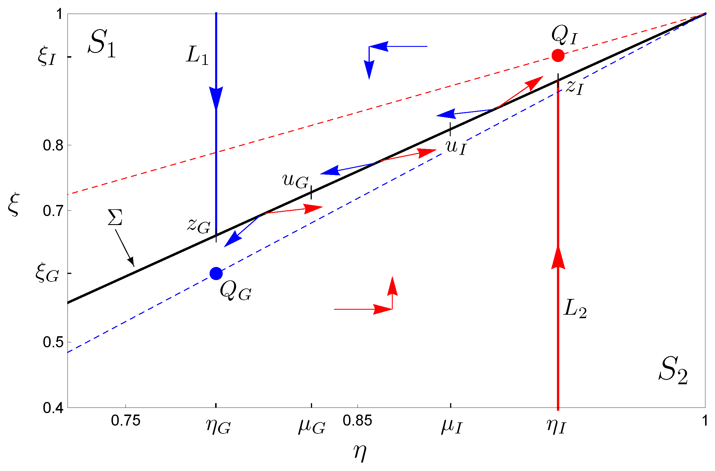
4. The Flip-Flop and Associated Filippov Flow

The theory of ODEs with discontinuous vector fields continues to advance, often based on the work of Filippov [27] and motivated in part by mathematical challenges arising in the modeling of systems that include phenomena such as switches and collisions [43,44]. In terms of our model, we preface the definition of the discontinuous vector field by first focusing on the diffusion coefficient D, which appears in each of the functions $f_{2i}\left(\eta \right),i>0$, in (13). It follows that the function $h\left(\eta \right)$ in (17) can be thought to be parametrized by D. Recall that an increase in D increases the efficiency of the meridional heat transport. We saw previously (Figure 2a) that an increase from $D=0.3$ to $D=0.394$ leads to a warmer world with a stable albedo line closer to the North Pole.

As mentioned in the Introduction, North put forth the possibility of using two D-values, with the smaller value corresponding to the ice-covered portion of the surface. While North only considered the fixed albedo line setting, system (19) has the advantage that the albedo- and ice-lines evolve with time. One might then imagine the value of D decreasing with an advancing ice sheet and increasing during a glacial retreat, playing its role in the negative feedback discussed in the Introduction. Here, we move to the discontinuous limit as it were, assuming a smaller constant value $D=D_G$ throughout the glacial advance, and a larger constant value $D=D_I$ throughout the retreat to an interglacial.

We will thus consider two climate regimes, one an “interglacial period” with $D=D_I=0.394$, and a “glacial period” for which $D=D_G=0.3$. We let $h_I\left(\eta \right)$ and $h_G\left(\eta \right)$ denote the function $h\left(\eta \right)$ in Equation (17) when $D=D_I$ and $D=D_G$, respectively. This represents step one in building the flip-flop characteristic of our model. We note the analysis to follow holds for any values $D_G<D_I$ for which there are distinct small stable ice cap equilibria.

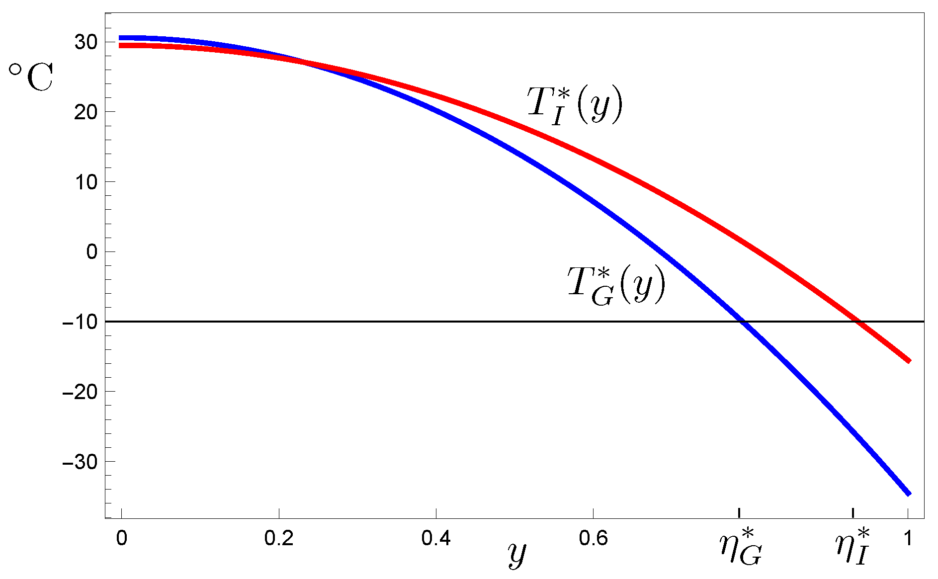
We pause before developing the model switching mechanism to revisit the positive ice albedo–temperature gradient feedback discussed in the Introduction. Let $\eta ={\eta }_G$ and $\eta ={\eta }_I$ denote the stable equilibrium solutions of Equation (17) when $D=D_G$ and $D=D_I$, respectively, as in Figure 2. Let $T_G^{\ast }\left(y\right)$ and $T_I^{\ast }\left(y\right)$ denote the corresponding equilibrium temperature profiles (14), which for $N=1$ are plotted in Figure 5. Note the temperature gradient during the glacial period ($\eta ={\eta }_G$) is larger than that during the interglacial period ($\eta ={\eta }_I$). We thus see that, at equilibrium, the model exhibits the desired effect associated with the positive ice albedo–temperature gradient feedback, namely, larger ice sheets due to enhanced poleward moisture transport brought on by an increased temperature gradient.

As for the switching mechanism from one climate state to the other, we recall the numerous studies mentioned above that indicate an increased ablation rate during glacial retreats is needed to simulate the glacial cycles in a qualitatively accurate manner. Our second step will be to select (dimensionless) ablation rates $b_G<b_I$ to incorporate this assumption. The two climate regimes are then modeled by the glacial advance system

$$\begin{array}{cc}\hfill \frac{d\eta }{dt}& =\frac{\rho }{R}{h}_G\left(\eta \right)\hfill \end{array}$$

(20a)

$$\begin{array}{cc}\hfill \frac{d\xi }{dt}& =\frac{ϵ}{R}(b_G(\eta -\xi )-a(1-\eta )),\hfill \end{array}$$

(20b)

and the interglacial system

$$\begin{array}{cc}\hfill \frac{d\eta }{dt}& =\frac{\rho }{R}{h}_I\left(\eta \right)\hfill \end{array}$$

(21a)

$$\begin{array}{cc}\hfill \frac{d\xi }{dt}& =\frac{ϵ}{R}(b_I(\eta -\xi )-a(1-\eta )).\hfill \end{array}$$

(21b)

We set $\mathcal{B}=\left\{\right(\eta ,\xi ):\eta \in [0,1],\xi \in [0,1\left]\right\}$, and we define the vector fields

$$V_G:\mathcal{B}\to {\mathbb{R}}^2,V_G(\eta ,\xi )=\left(\frac{\rho }{R}{h}_G\left(\eta \right),\frac{ϵ}{R}(b_G(\eta -\xi )-a(1-\eta ))\right)$$

and

$$V_I:\mathcal{B}\to {\mathbb{R}}^2,V_I(\eta ,\xi )=\left(\frac{\rho }{R}{h}_I\left(\eta \right),\frac{ϵ}{R}(b_I(\eta -\xi )-a(1-\eta ))\right).$$

Let ${\varphi }_G((\eta ,\xi ),t)$ and ${\varphi }_I((\eta ,\xi ),t)$ denote the flows associated with systems (20) and (21), respectively.

To switch climate regimes, we select a critical ablation parameter $b\in (b_G,b_I)$. When $b(\eta -\xi )-a(1-\eta )>0$ (i.e., the mass balance is negative), we assume the ice sheet is retreating and the system evolves according to (21). The system is in glacial advance mode when $b(\eta -\xi )-a(1-\eta )<0$ (i.e., the mass balance is positive). In this fashion, the set on which $b(\eta -\xi )-a(1-\eta )=0$, namely

$$\Sigma =\{(\eta ,\xi ):\xi =\gamma \left(\eta \right)=(1+\frac{a}{b})\eta -\frac{a}{b},\xi \in [0,1]\},$$

(22)

becomes a switching manifold (or discontinuity boundary) [45]. A trajectory for either system (20) or (21) that intersects $\Sigma$ in a crossing region switches to the alternate regime, as discussed in detail in Section 5. In spirit, this switching from one flow to the other is entirely analogous to that found in Welander’s mixed ocean layer model [28].

More formally, $\Sigma$ separates $\mathcal{B}$ into the domains

$$S_1=\{(\eta ,\xi )\in \mathcal{B}:\gamma \left(\eta \right)<\xi \}\mathrm{and}{S}_2=\{(\eta ,\xi )\in \mathcal{B}:\xi <\gamma \left(\eta \right)\}.$$

Note that each of $V_G$ and $V_I$ extend smoothly to $\Sigma$. For $x=(\eta ,\xi )\in \mathcal{B}$, consider the differential inclusion [45]

$$\frac{dx}{dt}\in V\left(x\right)=\left\{\begin{array}{cc}{V}_G\left(x\right),\hfill & x\in S_1\hfill \\ \{(1-q)V_G\left(x\right)+q{V}_I\left(x\right):q\in [0,1]\},\hfill & x\in \Sigma \hfill \\ V_I\left(x\right),\hfill & x\in S_2.\hfill \end{array}\right.$$

(23)

While in $S_1$ solutions have flow ${\varphi }_G$, while trajectories evolve under the flow ${\varphi }_I$ when in $S_2$. For $x\in \Sigma$, one assumes $dx/dt$ lies in the convex hull of the two vectors $V_G\left(x\right)$ and $V_I\left(x\right)$.

A solution to (23) in the sense of Filippov is an absolutely continuous function $x\left(t\right)$ satisfying $dx/dt\in V\left(x\right)$ for almost all t (note $x\left(t\right)$ is not differentiable at times t for which $x\left(t\right)$ enters or leaves $\Sigma$). As $V_G$ and $V_I$ are continuous on $\Sigma \cup S_1$ and $\Sigma \cup S_2$, respectively, the set-valued map $V\left(x\right)$ is upper semicontinuous, as well as closed, convex, and bounded for all $x\in \mathcal{B}$ and all $t\in \mathbb{R}$. These properties ensure that, for each $x_0\in \mathrm{Int}\left(\mathcal{B}\right)$, there is a solution $x\left(t\right)$ to differential inclusion (23) defined on an interval $[0,t_f]$ with $x\left(0\right)=x_0$ [45].

5. A Unique Nonsmooth Limit Cycle

5.1. Stable Virtual Equilibria

Let ${\psi }_G(\eta ,t)$ denote the flow associated with Equation (20a), and let ${\psi }_I(\eta ,t)$ denote the flow associated with Equation (21a). Recall that $h_G$ and $h_I$ are polynomials of degree $4N+3$, differing only in the choice of diffusion coefficients $D_G<D_I$.

The analysis of discontinuous system (23) is aided by the observation that the evolution of $\eta$ over time is independent of that of $\xi$. In particular, the Jacobian matrix for the vector field $V_G$ is

$$J_G=\left[\begin{array}{cc}\frac{\rho }{R}{h}_G^{\prime }\left(\eta \right)& 0\\ \frac{ϵ}{R}(b_G+a)& -\frac{ϵ}{R}{b}_G\end{array}\right]$$

(and similarly for the vector field $V_I$). As $-ϵb_G/R<0$ and $-ϵb_I/R<0$, the stability of any equilibrium solutions $(\eta ,\xi )$ of systems (20) and (21) will depend entirely on the signs of $h_G^{\prime }\left(\eta \right)$ and $h_I^{\prime }\left(\eta \right)$.

With $N=1$ and with parameter values as in Table 1, the degree seven polynomial $h_G\left(\eta \right)$ admits two equilibrium solutions ${\eta }_{G,u}\approx 0.197$ and ${\eta }_{G,s}\approx 0.789$ in the interval $[0,1]$, with $h_G^{\prime }\left({\eta }_{G,u}\right)>0$ and $h_G^{\prime }\left({\eta }_{G,s}\right)<0$ (see Figure 2). Thus, system (20) has a saddle $Q_{G,u}=({\eta }_{G,u},{\xi }_{G,u})$ and a stable node $Q_{G,s}=({\eta }_{G,s},{\xi }_{G,s})$. While ${\xi }_{G,u}<0$, the equilibrium $Q_{G,s}$ lies in $\mathcal{B}$ as ${\xi }_{G,s}\approx 0.641.$

As only the stable node for system (20) plays a role in the analysis, we let $Q_G$ and ${\eta }_G$ denote $Q_{G,s}$ and ${\eta }_{G,s}$, respectively, in all that follows.

Note the line

$$L_1=\{(\eta ,\xi ):\eta ={\eta }_G,\xi \in [0,1]\}$$

is invariant under the glacial flow ${\varphi }_G$, with solutions on $L_1$ converging monotonically to $Q_G$ over time. In addition, every ${\varphi }_G$-trajectory having initial condition in the region above $\Sigma$ and to the right of $L_1$, namely

$$S_1^{\prime }=\{(\eta ,\xi ):\eta \in [{\eta }_G,1],\gamma \left(\eta \right)<\xi \le 1\},$$

converges to $Q_G$ under the flow ${\varphi }_G$. This follows from the fact that a ${\psi }_G$-trajectory with initial condition ${\eta }_0\in [{\eta }_G,1]$ decreases monotonically to ${\eta }_G$ (recall Figure 2), and hence for such an ${\eta }_0$ the corresponding ${\varphi }_G$-trajectory of $({\eta }_0,{\xi }_0)$ satisfies $\xi \left(t\right)\to {\xi }_G$ due to the nature of Equation (20b).

Due to the ablation rate assumption $b_G<b$, note

$$(1+\frac{a}{b_G})\eta -\frac{a}{b_G}<(1+\frac{a}{b})\eta -\frac{a}{b}=\gamma \left(\eta \right)$$

(24)

for $\eta <1$. This implies that the $\xi$-nullcline for vector field $V_G$ lies below the switching manifold $\Sigma$. At points above the $\xi$-nullcline system, (20) satisfies $d\xi /dt<0$ (and $d\eta /dt<0$ for $\eta >{\eta }_G$); hence, ${\varphi }_G$-trajectories starting in $S_1^{\prime }$ move monotonically to the left and downward as they converge to $Q_G$ (see Figure 6).

Every ${\varphi }_G$-trajectory starting in $S_1^{\prime }$ will thus cross $\Sigma$ before approaching $Q_G$ and hence, following Filippov’s convention, switch to the interglacial flow ${\varphi }_I$ as the trajectory enters $S_2$. The fact the $\xi$-nullcline for system (20) lies below $\Sigma$ implies $Q_G$ is a virtual equilibrium point [43].

Definition 1.

Let$x\in \mathcal{B}$.

(i) x is a visible equilibrium point of (23) if either$V_G\left(x\right)=0$and$x\in S_1$, or if$V_I\left(x\right)=0$and$x\in S_2$.

(ii) x is a virtual equilibrium point of (23) if either$V_G\left(x\right)=0$and$x\in S_2$, or if$V_I\left(x\right)=0$and$x\in S_1$.

(iii) x is a boundary equilibrium point of (23) if$V_G\left(x\right)=V_I\left(x\right)=0$and$x\in \Sigma$.

We now consider the interglacial flow. With $N=1$ and with parameter values as in Table 1, the polynomial $h_I$ has three zeros ${\eta }_1\approx 0.22,{\eta }_2\approx 0.936$ and ${\eta }_3\approx 0.955$, with $h_I^{\prime }\left({\eta }_1\right)>0,h_I^{\prime }\left({\eta }_2\right)<0$ and $h_I^{\prime }\left({\eta }_3\right)>0$ (recall Figure 2). Thus, system (21) has two saddles (at which $\eta$ equals ${\eta }_1$ and ${\eta }_3$, respectively), with a stable node $Q_I=({\eta }_I,{\xi }_I)$ in-between. The line

$$L_2=\{(\eta ,\xi ):\eta ={\eta }_I,\xi \in [0,1]\}$$

is invariant under the flow ${\varphi }_I$, with ${\varphi }_I$-trajectories on $L_2$ converging monotonically to $Q_I$ over time.

The $\xi$-nullcline for vector field $V_I$ satisfies

$$(1+\frac{a}{b_I})\eta -\frac{a}{b_I}>\gamma \left(\eta \right)$$

for $\eta <1$ due to the assumption $b_I>b$, and hence lies above $\Sigma$. We thus have that $Q_I$ is a virtual equilibrium for the flow ${\varphi }_I$ since $Q_I\in S_1.$

Let $\Lambda$ denote the strip

$$\Lambda =\{(\eta ,\xi ):{\eta }_G\le \eta \le {\eta }_I,\xi \in [0,1]\},$$

and set ${\Lambda }_i=\Lambda \cap S_i,i=1,2$. Since $d\eta /dt>0$ and $d\xi /dt>0$ for system (21) in ${\Lambda }_2$, ${\varphi }_I$-trajectories starting in ${\Lambda }_2$ move monotonically to the right and upward as they approach $Q_I$, and hence must intersect and cross $\Sigma$. In this fashion, the systems “flip-flops" between glacial and interglacial periods in this region of phase space.

5.2. Tangencies on the Switching Manifold

To gain further insight into the Filippov flow, it is important to note where on $\Sigma$ the vector fields $V_G$ and $V_I$ are each tangent, given that such points may bound a sliding region [43]. To that end, a vector normal to $\Sigma$ is $\mathbf{N}={[1+\frac{a}{b}-1]}^T$. A computation yields $V_G·\mathbf{N}=0$ if and only if $h_G\left(\eta \right)=s_G\left(\eta \right)$, where

$$s_G\left(\eta \right)=\frac{aϵ(b_G-b)}{(a+b)\rho }(1-\eta ).$$

Note that the line $s_G$ has positive slope ($b_G-b<0)$, with $s_G\left(0\right)<0$ and $s_G\left(1\right)=0$. Recalling the plot of $h_G$ in Figure 2, the equation $h_G\left(\eta \right)=s_G\left(\eta \right)$ thus has a unique solution $\eta ={\mu }_G$ with ${\eta }_G<{\mu }_G$. Moreover, as $ϵ$ decreases to 0, ${\mu }_G$ will decrease monotonically toward ${\eta }_G$ as the line $s_G$ approaches the $\eta$-axis. One may check $V_G·\mathbf{N}>0$ at $x_1=(\eta ,\xi )\in \Sigma$ for which $\eta \in [{\eta }_G,{\mu }_G)$, so that $V_G$ points into $S_2$ at such $x_1$. Additionally, $V_G$ points into $S_1$ at $x_2=(\eta ,\xi )\in \Sigma$ for which $\eta \in ({\mu }_G,1]$, since $V_G·\mathbf{N}<0$ at such $x_2$ (see Figure 6).

Similarly, $V_I·\mathbf{N}=0$ if and only if $h_I\left(\eta \right)=s_I\left(\eta \right)$, where

$$s_I\left(\eta \right)=\frac{aϵ(b_I-b)}{(a+b)\rho }(1-\eta ),$$

a line with negative slope ($b_I-b>0)$ satisfying $s_I\left(0\right)>0$ and $s_I\left(1\right)=0$. Hence, $h_I\left(\eta \right)=s_I\left(\eta \right)$ has a unique solution $\eta ={\mu }_I\in ({\eta }_G,{\eta }_I)$, with ${\mu }_I$ increasing to ${\eta }_I$ as $ϵ$ decreases to 0. Moreover, $V_I$ points into $S_1$ at $x_1=(\eta ,\xi )\in \Sigma$ for which $\eta \in ({\mu }_I,{\eta }_I]$ (as $(V_I·\mathbf{N})\left(x_1\right)<0)$, while $V_I$ points into $S_2$ at $x_2=(\eta ,\xi )\in \Sigma$ for which $\eta \in [{\eta }_G,{\mu }_I)$ (as $(V_I·\mathbf{N})\left(x_2\right)>0)$.

In the analysis to follow, we choose $ϵ$ small enough to ensure ${\mu }_G<{\mu }_I$, which is possible given ${\eta }_G<{\eta }_I$. The points $u_G=({\mu }_G,\gamma \left({\mu }_G\right))$ and $u_I=({\mu }_I,\gamma \left({\mu }_I\right))$ on $\Sigma$ are known as invisible fold singularities [44]. This means the ${\varphi }_G$-trajectory passing through $u_G$ at $t=t_0$ is both tangent to $\Sigma$ at $u_G$ and contained in $S_2$ for t near $t_0$. Similarly, the ${\varphi }_I$-trajectory passing through $u_I$ is both tangent to $\Sigma$ at $u_I$ and contained in $S_1$ on some time interval.

Label the points $z_G=({\eta }_G,\gamma \left({\eta }_G\right))$ and $z_I=({\eta }_I,\gamma \left({\eta }_I\right))$ on $\Sigma$. The above discussion implies that ${\varphi }_I$-trajectories starting in ${\Lambda }_2$ cross $\Sigma$ moving to the right and up between $u_I$ and $z_I$, while ${\varphi }_G$-trajectories starting in ${\Lambda }_1$ cross $\Sigma$ between $z_G$ and $u_G$ moving to the left and down. The portions of $\Sigma$ between $z_G$ and $u_G$ and between $u_I$ and $z_I$ are known as crossing regions for the Filippov flow (23). As vector fields $V_G$ and $V_I$ are each smooth, Filippov solutions to differential inclusion (23) that pass through the crossing regions are unique.

The portion of $\Sigma$ between $u_G$ and $u_I$, known as a repelling sliding region [43], plays no role in the following analysis since Filippov trajectories beginning in ${\Lambda }_1,{\Lambda }_2$ or in one of the two crossing regions never intersect this sliding region.

5.3. The Filippov Return Map and a Unique Limit Cycle

Let $ϵ>0$ be chosen so that ${\mu }_G<{\mu }_I$. Let $J=[c,1],$ where ${\mu }_G<c\le {\mu }_I$. Let $I_1=\{(\eta ,\gamma \left(\eta \right)):\eta \in J\}$, and set $I_2=\{(\eta ,\gamma \left(\eta \right)):\eta \in [{\eta }_G,{\mu }_G]\}$. As shown in the preceding section, each ${\varphi }_G$-trajectory starting in $I_1$ crosses $\Sigma$ in $I_2$. For each $x\in I_1,$ there is a unique time $t_{ϵ}\left(x\right)$ such that ${\varphi }_G(x,t_{ϵ}\left(x\right))\in I_2$. For future reference, note $t_{ϵ}\left(x\right)\to \infty$ as $ϵ\to 0$. Define the mapping

$$r_{G,ϵ}:I_1\to I_2,x\mapsto {\varphi }_G(x,t_{ϵ}\left(x\right)).$$

Similarly, for each $x\in I_2$, there is a unique $t_{ϵ}\left(x\right)$ with ${\varphi }_I(x,t_{ϵ}\left(x\right))\in I_1,$ since the ${\varphi }_I$-trajectory of any such x crosses $\Sigma$ in $I_1$. This defines the map

$$r_{I,ϵ}:I_2\to I_1,x\mapsto {\varphi }_I(x,t_{ϵ}\left(x\right)).$$

The composition $r_{ϵ}=r_{I,ϵ}\circ r_{G,ϵ}:I_1\to I_1$ is then a continuous return map for the Filippov flow. Via our choice of the compact interval J, $r_{ϵ}$ has a fixed point in $I_1$ by Brouwer’s Fixed Point Theorem. This implies the existence of a (nonsmooth) periodic orbit $\Gamma$ for the Filippov system for any $ϵ>0$ for which ${\mu }_G<{\mu }_I$.

That the periodic orbit $\Gamma$ is unique and attracting for sufficiently small $ϵ$ is easily motivated. Note that, when $ϵ=0$, the ${\varphi }_G$-trajectory of $z_I=({\eta }_I,\gamma \left({\eta }_I\right))\in I_1$ limits on the regular equilibrium point $({\eta }_G,\gamma \left({\eta }_I\right))\in L_1$. Similarly, the ${\varphi }_I$-trajectory of $z_G=({\eta }_G,\gamma \left({\eta }_G\right))\in I_2$ limits on the regular equilibrium point $({\eta }_I,\gamma \left({\eta }_G\right))\in L_2$. For $ϵ$ sufficiently small, the periodic orbit $\Gamma$ is approximated by the rectangular “orbit” comprised of the ${\varphi }_G$-trajectory of $z_I$, the portion of $L_1$ from $({\eta }_G,\gamma \left({\eta }_I\right))$ down to $z_G$, the ${\varphi }_I$-trajectory of $z_G$, and the portion of $L_2$ back up to $z_I$ (akin to Figure 5 in [20]).

With this insight, the return map $r_{ϵ}:I_1\to I_1$ can be shown to be a contraction map as diam$\left(r_{ϵ}\left(I_1\right)\right)$ can be made as small as we please by decreasing $ϵ$ sufficiently, implying the existence of a unique fixed point to which all $r_{ϵ}$-orbits converge.

Theorem 1.

With parameters as in Table 1, there exists$\widehat{ϵ}>0$so that, for all$ϵ\in (0,\widehat{ϵ}]$, the Filippov system (23) admits a unique attracting limit cycle.

Proof. 

Let $c_1\in (0,1)$. Let $x=({\eta }_0,{\xi }_0)$ be any point in $I_1$. Recall ${\psi }_G\left({\eta }_0\right)\to {\eta }_G$ as $t\to \infty$, where ${\psi }_G$ is the flow associated with ODE (20a), here with initial condition ${\psi }_G\left(0\right)={\eta }_0$. As the interval J used to define $I_1$ is compact, there exists a time $T_1$ so that for all $t\ge T_1,$ for all ${\eta }_1,{\eta }_2\in J,|{\psi }_G\left({\eta }_1\right)-{\psi }_G\left({\eta }_2\right)|\le c_1|{\eta }_1-{\eta }_2|$.

Given $x\in I_1$, pick $ϵ\left(x\right)>0$ so that $t_{ϵ\left(x\right)}\left(x\right)>T_1$ (recalling ${\varphi }_G(x,t_{ϵ\left(x\right)}\left(x\right))\in I_2$). By the continuity of ${\varphi }_G$ with respect to initial conditions and time, there exists $\delta =\delta \left(x\right)>0$ so that, for all $y\in B_{\delta \left(x\right)}\cap I_1$, $t_{ϵ\left(x\right)}\left(y\right)>T_1$, where $r_{G,ϵ\left(x\right)}\left(y\right)\in I_2.$ Note that, for any $ϵ\le ϵ\left(x\right),t_{ϵ}\left(y\right)>T_1$ for $y\in B_{\delta \left(x\right)}\cap I_1$.

Letting x vary in $I_1$ leads to an open cover

$$I_1\subset \bigcup _{x\in I_1}{B}_{\delta \left(x\right)}\left(x\right)$$

of the compact set $I_1$. Let $\{B_{\delta \left(x_i\right)}\left(x_i\right):i=1,\cdots ,n\}$ be a finite subcover, and set ${ϵ}_1=min\{ϵ\left(x_i\right):i=1,\dots ,n\}$. Then, for any $ϵ\le {ϵ}_1$ and for all $x\in I_1,t_{ϵ}\left(x\right)>T_1$.

Now, let $ϵ\le {ϵ}_1,$ let $x_1=({\eta }_1,\gamma \left({\eta }_1\right))$ and $x_2=({\eta }_2,\gamma \left({\eta }_2\right))$ be points in $I_1$, and set $r_{G,ϵ}\left(x_1\right)=({\eta }_1^{\prime },\gamma \left({\eta }_1^{\prime }\right))=x_1^{\prime }$ and $r_{G,ϵ}\left(x_2\right)=({\eta }_2^{\prime },\gamma \left({\eta }_2^{\prime }\right))=x_2^{\prime }$. Note that

$$|{\eta }_1^{\prime }-{\eta }_2^{\prime }{|}^2\le c_1^2{|{\eta }_1-{\eta }_2|}^2.$$

via the assumption $ϵ\le {ϵ}_1$. We have

$$\begin{array}{cc}\hfill \parallel r_{G,ϵ}(x_1)-r_{G,ϵ}(x_2){\parallel }^2& =|{\eta }_1^{\prime }-{\eta }_2^{\prime }{|}^2+{(\gamma ({\eta }_1^{\prime })-\gamma ({\eta }_2^{\prime }))}^2\hfill \\ \hfill & =|{\eta }_1^{\prime }-{\eta }_2^{\prime }{|}^2+{(1+\frac{a}{b})}^2{|{\eta }_1^{\prime }-{\eta }_2^{\prime }|}^2\hfill \\ \hfill & \le c_1^2|{\eta }_1-{\eta }_2|+{(1+\frac{a}{b})}^2{c}_1^2{({\eta }_1-{\eta }_2)}^2\hfill \\ \hfill & =c_1^2|{\eta }_1-{\eta }_2|+c_1^2{(\gamma ({\eta }_1)-\gamma ({\eta }_2))}^2\hfill \\ \hfill & =c_1^2{\parallel x_1-x_2\parallel }^2.\hfill \end{array}$$

In a similar fashion, given $c_2\in (0,1)$, there exists ${ϵ}_2$ such that for all $ϵ\in (0,{ϵ}_2)$, and for all $x_1$ and $x_2$ in $I_2,\parallel r_{I,ϵ}(x_1)-r_{I,ϵ}(x_2)\parallel \le c_2\parallel x_1-x_2\parallel$.

Now, note that, for $ϵ\in (0,\widehat{ϵ}]$, where $\widehat{ϵ}=min\{{ϵ}_1,{ϵ}_2\}$, the return map $r_{ϵ}:I_1\to I_1$ is a contraction map with contraction factor $c_1{c}_2$. □

The attracting limit cycle $\Gamma$ is illustrated in Figure 7, along with plots of $\eta ,\xi$ and the ice sheet mass balance evolving with time. Other than for a slightly reduced period of oscillation when $N=3$ (Figure 7b, which has the same time scale as Figure 7a), we again note the quadratic and higher-order approximations yield qualitatively similar dynamics.

With parameter values as in Table 1, recall ODE (21a) has an unstable equilibrium ${\eta }_{I,u}$ lying between the stable equilibrium ${\eta }_I$ and the North Pole. The line

$$L_3=\{(\eta ,\xi ):\eta ={\eta }_{I,u}\}$$

(25)

is invariant under the interglacial flow ${\varphi }_I$, with each ${\varphi }_I$-trajectory on $L_3$ converging to $Q_{I,u}=({\eta }_{I,u},{\xi }_{I,u})$ in forward time. Thus, any point $x=(\eta ,\xi )\in S_2$ with ${\eta }_G\le \eta \le {\eta }_{I,u}$ will be in the stable set of the unique attracting limit cycle $\Gamma$, since the trajectory ${\varphi }_I(x,t)$ must intersect $I_1$. At points $x=(\eta ,\xi )$ in $S_2$ and to the right of $L_3$, however, vector field $V_I$ points to the right. Hence, a ${\varphi }_I$-trajectory with initial condition x may hit the boundary $\eta =1$ prior to intersecting $\Sigma$, and thus would not converge to $\Gamma$. We comment further on trajectories intersecting the boundary of $\mathcal{B}$ in the concluding section.

The small unstable ice cap exists due to the choice $D=D_I=0.394$. As D decreases from $D_I=0.394$, the small unstable ice cap disappears, as can be gleaned from the bifurcation plot in Figure 3, with the ice-free Earth moving from “stable” to “unstable” as D decreases. If $D_I$ were chosen so that the small unstable ice cap equilibrium at ${\eta }_{I,u}$ did not exist, the stable set of the unique attracting limit cycle $\Gamma$ would include all $x=(\eta ,\xi )\in \mathcal{B}$ with $\eta$ greater than the $\eta$-value corresponding to the large unstable interglacial ice cap.

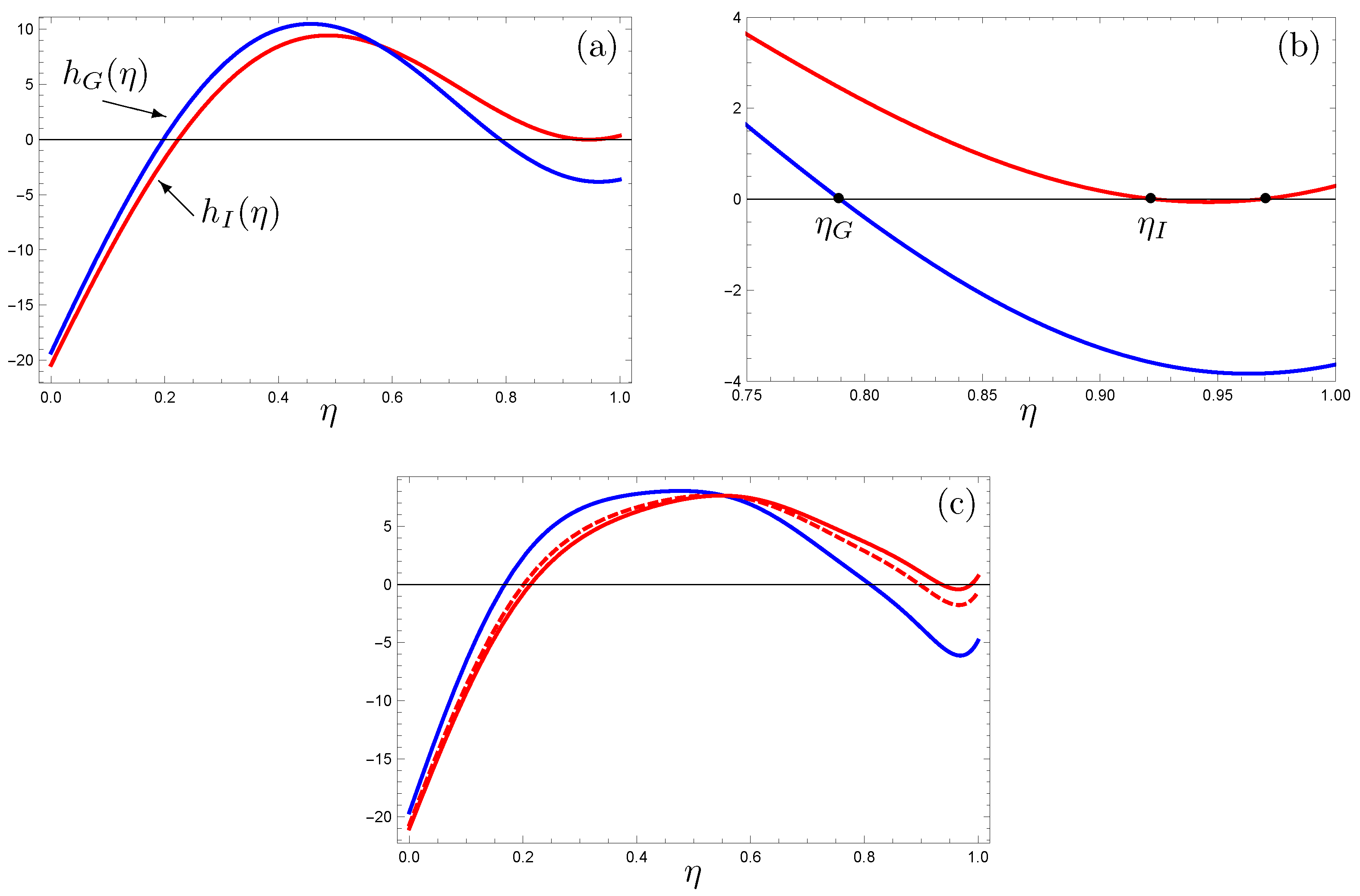
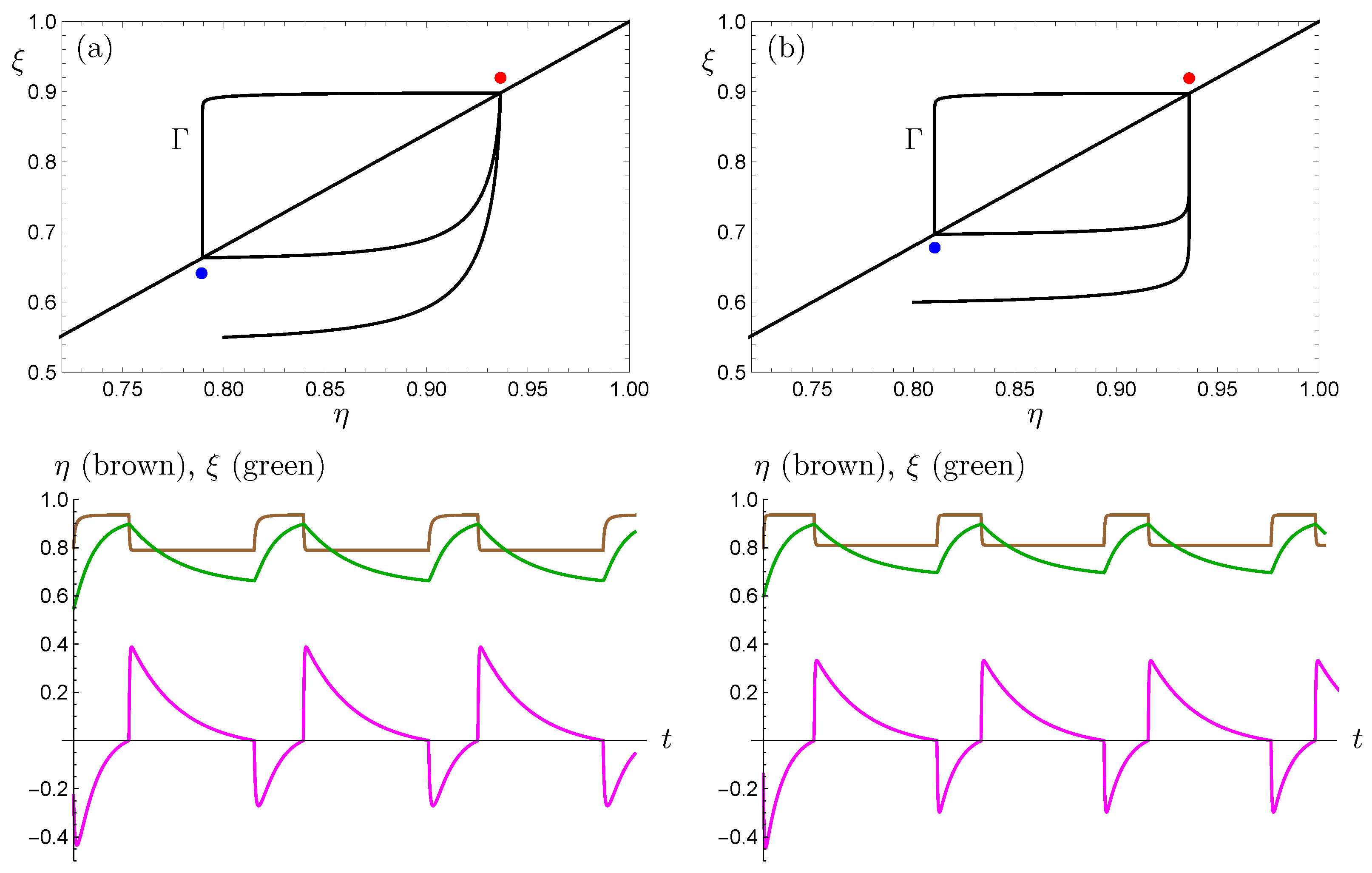
6. Feedbacks and Meridional Flux at the Albedo Line

Placing the limit cycle depicted in Figure 7 in the context of the climate feedbacks discussed in the Introduction, we consider first the glacial advance. At the onset of the glacial age, the albedo in the polar region increases, leading to a steeper temperature gradient. This in turn enhances the meridional transport of moisture to northern latitudes where it precipitates out as snow, leading to further ice sheet growth. The albedo line $\eta$ descends and, over time, the ice edge $\xi$ follows, with the ice sheet mass balance positive in this regime.

As the ice edge descends, the assumption of reduced meridional transport efficiency comes into play, inhibiting the positive ice albedo–temperature gradient feedback. Accumulation on the ice sheet is reduced and eventually comes to a halt, while inertia keeps the ice edge $\xi$ from responding quickly [9]. Thus, the ablation zone between $\xi$ and $\eta$ expands prior to the retreat, as is the case with the large model presented in [2].

The expansion of the ablation zone triggers the switch to the interglacial state as the mass balance becomes negative. In this mode, transport efficiency is increased, whereas the meridional temperature gradient is reduced. The albedo line moves poleward with the ice edge slowly following. The effect of the increase in the diffusion coefficient can be seen in the fact the albedo line stops its retreat shy of the North Pole as, eventually, snow again begins to precipitate out and the cycle begins anew.

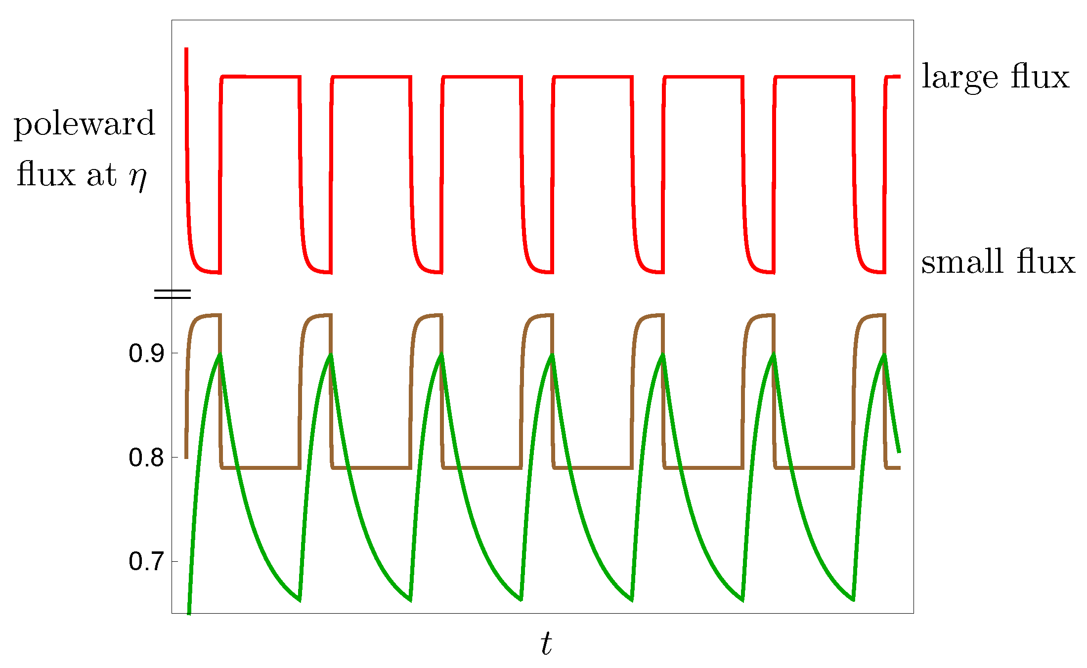
The behavior described above can be summarized by considering the total meridional heat flux across the albedo line $\eta$ over time. The flux at $\eta$ is computed by integrating the diffusive heat transport term in (1) with respect to y, while making use of expression (7) for the temperature. The total heat flux moving poleward across latitude y is proportional to

$$D(1-y^2)\sum _{i=1}^N{T}_{2i}{P}_{2i}^{\prime }(y).$$

(26)

Using the assumption $T_{2i}=f_{2i}(\eta )$ for each i and evaluating (26) at $\eta$ yields

$$\ell (\eta )=D(1-{\eta }^2)\sum _{i=1}^N{f}_{2i}(\eta )P_{2i}^{\prime }(\eta ).$$

(27)

Expression (27) is then proportional to the total meridional heat flux across $\eta$.

The plot of $\ell (\eta )$ is shown in Figure 8. Note the increase in the poleward flux at $\eta$ coincides with the advance of the albedo line. Due to the associated extensive ice cover, the transport efficiency is reduced, and, while the ice sheet edge continues to descend, the flux and the albedo line remain steady. When the system flips to the interglacial state, the poleward flux at $\eta$ decreases as the albedo line retreats. Although the temperature gradient now weakens, the increased efficiency ensures moisture reaches northern latitudes, and eventually the albedo line stabilizes with the ice edge retreating. This simple flip-flop model serves to illuminate the interplay between the two competing feedbacks.

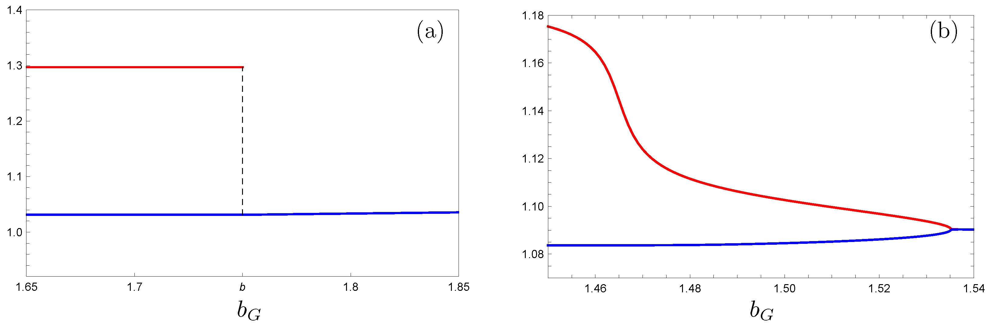
7. Bifurcation Scenarios

Recall that the ablation rates were chosen to satisfy $b_G<b<b_I$. As $b_G$ increases to b, the $V_G$ $\xi$-nullcline approaches the switching boundary $\Sigma$ (see Figure 6 and Equation (24)). When $b_G=b$, the equilibrium point $Q_G$ lies on $\Sigma$; when $b_G>b$, $Q_G$ lies in $S_1$ and thus becomes a visible equilibrium. Similarly, $Q_I$ can be made to pass through $\Sigma$ by letting $b_I$ decrease through b.

As $b_G$ increases through b, the limit cycle $\Gamma$ is lost through a border collision bifurcation [44], a type of nonsmooth Hopf bifurcation. For $b_G>b$, a trajectory starting in ${\Lambda }_1$ will converge to $Q_G$, never intersecting $\Sigma$ and so never triggering the flip-flop. In Figure 9a, we plot the limiting maximum and minimum values of the norm of trajectories beginning in ${\Lambda }_1$ as $b_G$ passes through b (assuming $ϵ$ is sufficiently small).

Figure 9b presents an associated smooth Hopf bifurcation in which the instantaneous switching from $b_G$ to $b_I$ and from $D_G$ to $D_I$ are replaced by smooth transitions. For the simulations presented here, the parameter b in Equation (19b) is replaced by the expression

$$H(s)=\frac{1}{2}(b_G+b_I)-\frac{1}{2}(b_G-b_I)tanh(Ms),$$

(28)

with s replaced by the negative of the mass balance term, $b(\eta -\xi )-a(1-\eta )$. Similarly, replacing $b_G$ and $b_I$ in (28) with $D_G$ and $D_I$, respectively, leads to a smooth transition between the glacial advance and retreat diffusion constants. In this way, system (19) becomes a smooth dynamical system that approximates our flip-flop model for large M-values.

We again vary $b_G$, but now in the smooth $(\eta ,\xi )$-system. The plot in Figure 9b displays the existence of a stable (spiral) equilibrium for $b_G$ larger than roughly 1.535. For $b_G<1.535$, there is a stable limit cycle created through a supercritical Hopf bifurcation, with the maximum (red) and minimum (blue) values of the norm on the limit cycle plotted as a function of $b_G$. The existence of a Hopf bifurcation has played an important role in other models of the glacial cycles; see, for example, [10,46].

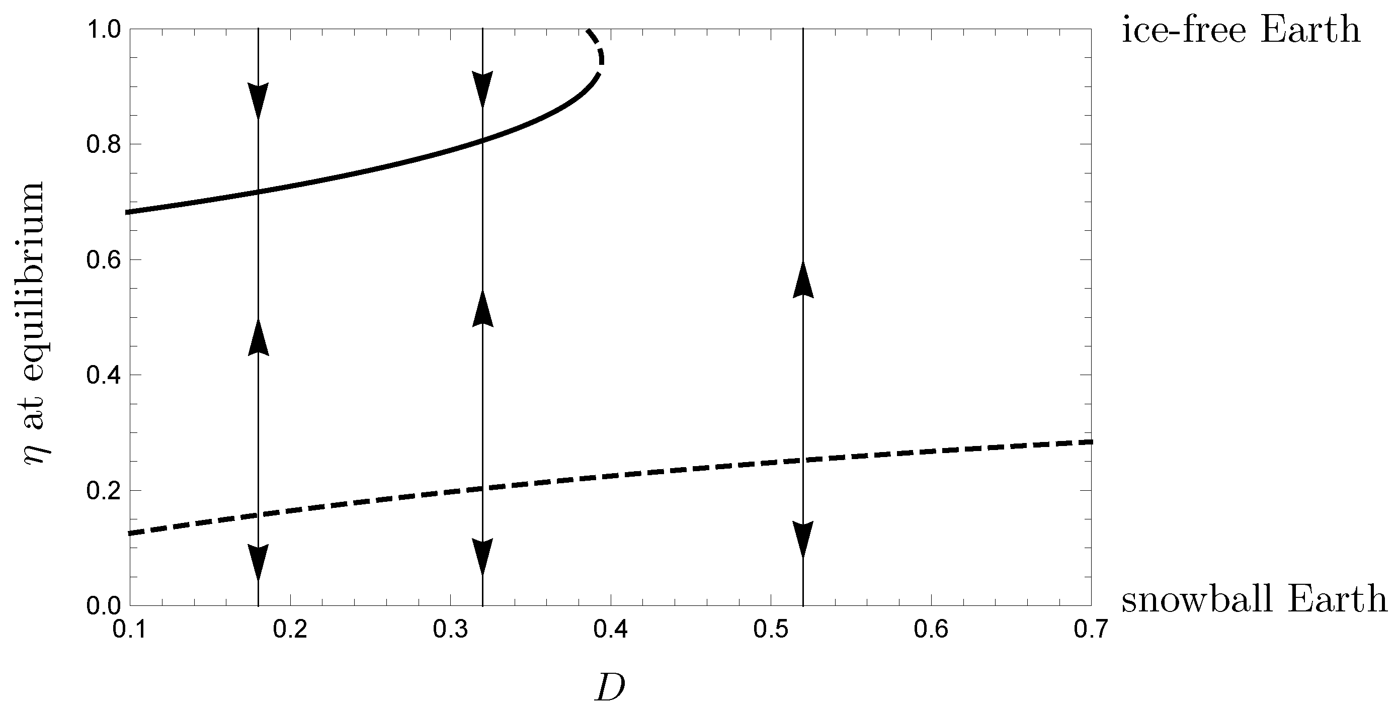
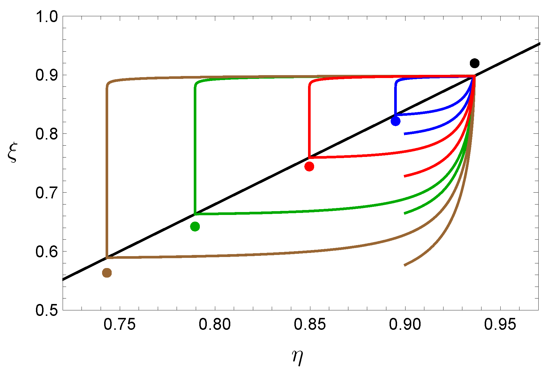
Returning to the discontinuous model, one can also vary the diffusion constant parameters. For example, the choice of $D_G$ determines the extent of the glacial state ice cap: reducing $D_G$ leads to larger ice caps (recall Figure 1). Varying $D_G$ then leads to limit cycles with larger amplitude and period (Figure 10), akin in spirit to the behavior associated through the MPT.

Welander’s mixed ocean layer flip-flop model [28] was placed in the nonsmooth setting and analyzed in [47]. The periodic orbit in the Filippov analysis of Welander’s equations arises in a nonsmooth Hopf bifurcation through a fused focus [27] as a parameter is varied. We note that the corresponding bifurcation in our model is entirely analogous.

Recall that there is a repelling sliding region between the invisible fold singular points $u_G$ and $u_I$ on $\Sigma$, assuming the time constant $ϵ$ for the evolution of the ice edge $\xi$ is sufficiently small. As $ϵ$ is increased, $u_G$ and $u_I$ merge in a double invisible tangency point (what Filippov termed a fused focus) and then pass each other, with an attracting sliding region now on $\Sigma$ between $u_I$ and $u_G$ and no periodic orbit. This is the same type of bifurcation exhibited by Welander’s model and presented in [47].

While simple in nature, the model presented here exhibits relatively rich dynamical behavior.

8. Forcing with Milankovitch Cycles

The eccentricity e of the Earth’s orbit, which varies with a period of roughly 100,000 years, has an effect on the amount of insolation reaching the planet and thus on climate on geologic time scales. The global annual average insolation as a function of e is

$$Q=Q(e)=\frac{Q_0}{\sqrt{1-e^2}},$$

(29)

where $Q_0$ is the insolation value corresponding to $e=0$ [11]. The magnitude of the change in Q due to eccentricity is roughly $0.6$ W/m${}^2$. This change in incoming solar radiation by itself is too weak to account for the glacial-interglacial global temperature changes [5].

The obliquity $\beta$ of the Earth’s spin axis plays an important role in our climate over geologic time. The obliquity varies with a period of about 41,000 years, ranging between roughly 22${}^{\circ }$ and 24.5${}^{\circ }$. For smaller $\beta$-values, less insolation is received in the polar regions, leading to an increased temperature gradient. This scenario is then favorable for the growth of a polar ice cap. Conversely, greater insolation is received in the polar regions for larger $\beta$-values, leading to a decreased temperature gradient. This scenario is thus favorable for the potential retreat of a large ice sheet. The roles of eccentricity and obliquity—and precession, if seasons are considered—in influencing the Earth’s glacial-interglacial history have been well-studied (see, for example, [17,23,48]).

Recall that the insolation latitudinal distribution function (2) depends upon $\beta .$ In [36], a mechanism to compute $s(y,\beta )$ as a polynomial in both y and $\beta$, to any desired degree of accuracy, is presented. As discussed in [36], the second degree expansion

$$s(y,\beta )=1-\frac{5}{8}{P}_2(cos\beta )P_2(y)$$

(30)

well approximates Equation (2) for planets with obliquity values similar to Earth’s.

We incorporate (29) and (30) into the Filippov system (23), using values of e and $\beta$ computed by Laskar [22]. A difficulty that arises immediately is the proximity of the (interglacial) small, saddle ice cap equilibrium to the stable node $({\eta }_I,{\xi }_I)$ when $D=0.394$ (Figure 2b). In every simulation run with Milankovitch forcing, the ${\varphi }_I$-trajectory shoots poleward of the stable manifold (25) of the small ice cap saddle and heads to the boundary $\eta =1$. We thus use the reduced value $D_G=0.38$, for which there is no small ice cap saddle equilibrium (recall Figure 3), for this simulation.

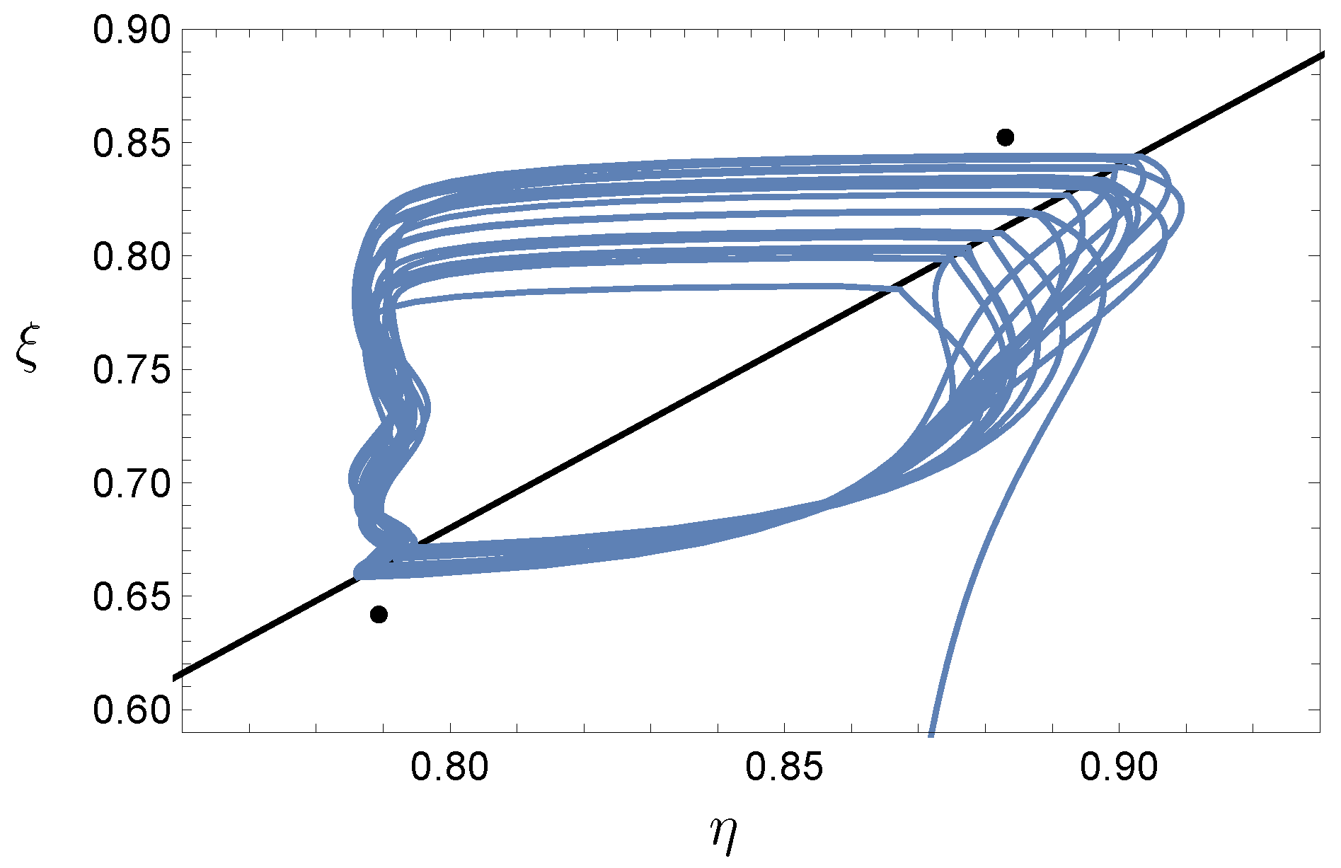
Results of a representative solution are shown in Figure 11 and Figure 12. Note the trajectory continues to pass through the discontinuity boundary when in both glacial and interglacial modes, thereby producing the glacial cycles. The top image in Figure 12 shows the behavior of $\eta$ and $\xi$ over the past 1 million years, that is, through the past 10 model glacial cycles. The effect of Milankovitch forcing is clearly evident in the plot of the albedo line $\eta$.

The lower plot in Figure 12 displays the meridional flux at the albedo line $\ell (\eta )$ (27) (red, scaled and translated), as well as the obliquity $\beta$ (blue). We focus on the obliquity as the magnitude of the change in insolation due to time-varying eccentricity is too small to account for the glacial-interglacial global climate changes, as mentioned above. We also note the emphasis here is placed on $\eta$ rather than $\xi$ as it is the albedo line (or snow line) that principally drives the model dynamics, due to its role in the competing feedbacks discussed in the introduction.

Note that maximum and minimum $\beta$-values correspond to minimum and maximum values, respectively, of $\ell (\eta )$. This is consistent with the fact that smaller $\beta$-values lead to larger temperature gradients and increased meridional transport, while larger $\beta$-values lead to reduced temperature gradients and diminished meridional transport.

Huybers argued in [17] that high obliquity is essential for the initiation of a glacial retreat. Indeed, the dominant signal seen in the climate data prior to the MPT is obliquity, as mentioned previously. Huybers also noted that after the MPT the climate data indicate that at times two maximum $\beta$-values are skipped before initiation of a deglaciation. He further posited that perhaps the 100 kyr cycles after the MPT are the average of 80 kyr (two $\beta$-cycles per glacial cycle) and 120 kyr (three $\beta$-cycles per glacial cycle).

Huyber’s proposition is supported by the model output. As can be seen in the lower plot in Figure 12, one half of the model glacial cycles skip two maximum $\beta$-values. Correspondingly, the flux at the albedo line passes through two minimum values during one half of the ten glacial cycles in Figure 12, prior to decreasing to the the flux value at $\eta$ during an interglacial. The conceptual model introduced here illustrates Huyber’s concept quite well, while bringing the poleward flux at $\eta$ in response to obliquity forcing into play in a novel way.

9. Discussion and Future Work

We have introduced a new conceptual model of the glacial cycles, with an energy balance annual and zonal mean surface temperature equation with diffusive heat transport (1) the starting point. We recast the coupled dynamic ice line introduced in [15] as the albedo line, entirely consistent with Budyko’s piecewise-constant albedo function (3). As in [20], the new ice edge variable $\xi$ is incorporated to allow for consideration of ablation and accumulation zones on the ice sheet.

The present work differs from [20] in several important regards. The meridional transport term used in [20] is Budyko’s relaxation to the mean term (5). The associated zonal average surface temperature equation again presents an infinite dimensional dynamical system, one which is approximated in a manner far different from that used here in Section 3 [12]. Lacking a diffusive process, it is the critical temperature $T_c$ that is varied between glacial and interglacial states in [20]. One motivation for this choice was provided by [8], in which the value of $T_c$ was assumed to depend upon changes in the deep ocean temperature.

The model presented here was strongly motivated by work of Raymo and Nisancioglu [23], in which competing feedbacks associated with meridional transport and related to ice-albedo feedback are discussed in depth. It is natural to connect these feedbacks with poleward flux, as we have done here, which then leads to consideration of a diffusive transport term.

We note the use of diffusive heat transport smooths the albedo function discontinuity in the sense the temperature profile is continuous (Figure 5; this is not the case when using transport term (5)). The discontinuity in our model vector field arises from the use of a larger ablation rate during interglacial retreats, and a switching mechanism motivated by mass balance principles as in [20].

The model focuses on the interplay of feedbacks associated with ice-albedo feedback, namely, the temperature gradient (positive) and transport efficiency (negative) feedbacks, similar in spirit to considerations in [23]. We assume a large ice sheet results in less efficient heat transport, and hence we use a smaller “glacial” parameter $D_G$ than “interglacial” parameter $D_I$.

An ad hoc method is used to analyze the resulting nonsmooth geometric singular perturbation problem. A nonsmooth attracting limit cycle is shown to exist, provided the ice edge moves slowly enough. The model oscillations continue when forced by time-varying obliquity and eccentricity values. We note the competing feedbacks mentioned above serve to determine the maximal ice sheet size.

Many questions of a mathematical nature are raised by this flip-flop glacial cycle model. It would be of interest to extend the analysis presented here to the boundary of $\mathcal{B}$, particularly the segments $\eta =1$ and $\xi =1$. The Filippov flow would have to be extended to include this portion of state space, perhaps along the lines of work by Barry et al. in [16].

Interesting questions concerning bifurcations would then arise for the extended flow and a state space that includes the boundary of $\mathcal{B}$. What becomes of the saddle-node bifurcation indicated in Figure 3 with dynamics defined on the line $\eta =1$? In addition, an investigation of model dynamics in the case of the small unstable ice cap scenario (Figure 2b) would then be of interest when subjected to Milankovitch forcing, which can push trajectories poleward toward $\eta =1$ as discussed previously.

Another intriguing problem concerns making, say, the stable equilibrium $Q_G$ visible and placing it near or on the discontinuity boundary $\Sigma$, and then determining the effect of Milankovitch forcing in this situation. Might Milankovitch forcing push the system to tip over to the interglacial mode, and how might any such tipping depend upon the time constant $ϵ$ for the ice sheet edge?

We also note the work presented here is the first part of a larger project aimed at investigating the Pliocene-Pleistocene Transition (PPT) via our mathematical model. The PPT refers to the development of perennial sea and land ice in the Northern Hemisphere, of an eventual extent similar to that which we have today. The study [49] used ocean cores drilled at the present Arctic Ocean summer ice margin to reconstruct the local climate during this transition. The following findings come from this work.

Roughly 5 Mya (million years ago) the Arctic Ocean was ice free at the drilling site, or covered by first-year winter ice. Sea ice expanded from the central Arctic Ocean for the first time about 4 Mya, at a time when atmospheric CO${}_2$ levels were similar to today’s and the global average temperature was 1–2 ${}^{\circ }$C warmer than at present. This early Pliocene climate is often viewed as an analog of a future warmer Earth.

Not until about 2.6 Mya, during the PPT, did Arctic Sea ice expand to its modern winter limits. The glacial cycle model presented here concerns the Earth’s climate from this point to the present.

A long-term decrease in atmospheric CO${}_2$ concentration accompanied the amplification of the polar cooling described above through the PPT. The parameter A in (1) is often used as a proxy for the concentration of greenhouses gases such as atmospheric CO${}_2$: larger CO${}_2$ values lead to reduced OLR (a decrease in A), and smaller CO${}_2$ concentrations lead to increased OLR (an increase in A).

Our model can be enhanced by taking A to be a dynamic variable, similar to the work of Barry et al. in [16]. Consideration of an ice-free state would entail an analysis of system (23) on the boundary $\eta =1$ or $\xi =1$. Either scenario might be associated with a decrease in CO${}_2$, that is, an increase in A, as atmospheric CO${}_2$ is drawn down by a silicate weathering process [50] enhanced by the lack of ice cover. In future work, the idealized mathematical model presented here will be extended in an effort to gain insight into the interactions of the large scale mechanisms and feedbacks in play through the PPT.

References

1. Imbrie, J.; Imbrie, K. Ice Ages; Harvard University Press: Cambridge, MA, USA, 1979. [Google Scholar]
2. Abe-Ouchi, A.; Saito, F.; Kawamura, K.; Raymo, M.E.; Okuno, J.; Takahashi, K. Insolation-driven 100,000-year glacial cycles and hysteresis of ice-sheet volume. Nature 2013, 500, 190–194. [Google Scholar] [CrossRef] [PubMed]
3. PalMod, German Climate Modeling Initiative. Available online: https://www.palmod.de/ (accessed on 20 February 2020).
4. Raymo, M.E.; Lisiecki, L.E.; Nisancioglu, K. Plio-Pleistocene ice volume, Antarctic climate, and the global δ18O record. Science 2006, 313, 492–495. [Google Scholar] [CrossRef] [PubMed]
5. Brook, E.; Buizert, C. Antarctic and global climate history viewed from ice cores. Nature 2018, 558, 200–208. [Google Scholar] [CrossRef] [PubMed]
6. Ashwin, P.; Ditlevsen, P. The middle Pleistocene transition as a generic bifurcation on a slow manifold. Clim. Dynam. 2015, 45, 2683–2695. [Google Scholar] [CrossRef] [Green Version]
7. Budyko, M.I. The effect of solar radiation variation on the climate of the Earth. Tellus 1969, 5, 611–619. [Google Scholar]
8. Gildor, H.; Tziperman, E. A sea ice climate switch mechanism for the 100-kyr glacial cycles. J. Geophys. Res 2001, 106, 9117–9133. [Google Scholar] [CrossRef]
9. Källén, E.; Crafoord, C.; Ghil, M. Free oscillations in a climate model with ice-sheet dynamics. J. Atmos. Sci. 1979, 36, 2292–2303. [Google Scholar] [CrossRef]
10. Maasch, K.; Saltzman, B. A low-order dynamical model of global climatic variability over the full Pleistocene. J. Geophys. Res. 1990, 95, 1955–1963. [Google Scholar] [CrossRef]
11. McGehee, M.; Lehman, C. A paleoclimate model of ice-albedo feedback forced by variations in Earth’s orbit. SIAM J. Appl. Dyn. Syst. 2012, 11, 684–707. [Google Scholar] [CrossRef]
12. McGehee, M.; Widiasih, E. A quadratic approximation to Budyko’s ice-albedo feedback model with ice line dynamics. SIAM J. Appl. Dyn. Syst. 2014, 13, 518–536. [Google Scholar] [CrossRef]
13. Parrenin, F.; Paillard, D. Amplitude and phase of glacial cycles from a conceptual model. Earth Planet. Sci. Lett. 2003, 214, 243–250. [Google Scholar] [CrossRef]
14. Sellers, W. A global climatic model based on the energy balance of the Earth-Atmosphere system. J. Appl. Meteor. 1969, 8, 392–400. [Google Scholar] [CrossRef]
15. Widiasih, E. Dynamics of the Budyko energy balance model. SIAM J. Appl. Dyn. Syst. 2013, 12, 2068–2092. [Google Scholar] [CrossRef] [Green Version]
16. Barry, A.; Widiasih, E.; McGehee, R. Nonsmooth frameworks for an extended Budyko model. Disc. Cont. Dyn. Syst. B 2017, 22, 2447–2463. [Google Scholar] [CrossRef]
17. Huybers, P. Glacial variability over the last two million years: An extended depth-derived agemodel, continuous obliquity pacing, and the Pleistocene progression. Quat. Sci. Rev. 2007, 26, 37–55. [Google Scholar] [CrossRef] [Green Version]
18. Paillard, D. The timing of Pleistocene glaciations from a simple multiple-state climate model. Nature 1998, 391, 378–381. [Google Scholar] [CrossRef]
19. Paillard, D.; Parrenin, F. The Antarctic ice sheet and the triggering of deglaciations. Earth Planet. Sc. Lett. 2004, 227, 263–271. [Google Scholar] [CrossRef]
20. Walsh, J.A.; Widiasih, E.; Hahn, J.; McGehee, R. Periodic orbits for a discontinuous vector field arising from a conceptual model of glacial cycles. Nonlinearity 2016, 29, 1843–1864. [Google Scholar] [CrossRef] [Green Version]
21. Hays, J.D.; Imbrie, J.; Shackleton, N.J. Variations in the Earth’s orbit: pacemaker of the ice ages. Science 1976, 4270, 1121–1132. [Google Scholar] [CrossRef]
22. Laskar, J.; Fienga, A.; Gastineau, M.; Manche, H. La2010: A new orbital solution for the long-term motion of the Earth. Astron. Astrophys. 2011, 532, A89. [Google Scholar] [CrossRef]
23. Raymo, M.E.; Nisancioglu, K. The 41 kyr world: Milankovitch’s other unsolved mystery. Paleoceanography 2003, 18. [Google Scholar] [CrossRef] [Green Version]
24. North, G. Theory of energy-balance climate models. J. Atmos. Sci. 1975, 32, 2033–2043. [Google Scholar] [CrossRef] [Green Version]
25. Pierrehumbert, R.T.; Abbot, D.S.; Voigt, A.; Koll, D. Climate of the Neoproterozoic. Ann. Rev. Earth Planet. Sci. 2011, 39, 417–460. [Google Scholar] [CrossRef] [Green Version]
26. Fenichel, N. Persistence and smoothness of invariant manifolds for flows. Indiana U. Math. J. 1971, 21, 193–226. [Google Scholar] [CrossRef]
27. Filippov, A.F. Differential Equations with Discontinuous Righthand Sides; Kluwer Academic Publishers: Dordrecht, The Netherlands, 1988. [Google Scholar]
28. Welander, P. A simple heat-salt oscillator. Dyn. Atmos. Oceans 1982, 6, 233–242. [Google Scholar] [CrossRef]
29. North, G. Analytic solution to a simple climate with diffusive heat transport. J. Atmos. Sci. 1975, 32, 1301–1307. [Google Scholar] [CrossRef] [Green Version]
30. North, G. The small ice cap instability in diffusive climate models. J. Atmos. Sci. 1984, 41, 3390–3395. [Google Scholar] [CrossRef] [Green Version]
31. North, G.; Cahalan, R.; Coakley, J. Energy balance climate models. Rev. Geophys. Space Phys. 1981, 19, 91–121. [Google Scholar] [CrossRef] [Green Version]
32. Schwartz, S. Heat capacity, time constant, and sensitivity of Earth’s climate system. J. Geophys. Res. 2007, 112, D24S05. [Google Scholar] [CrossRef]
33. Graves, C.; Lee, W.-H.; North, G. New parameterizations and sensitivities for simple climate models. J. Geophys. Res. 1993, 98, 5025–5036. [Google Scholar] [CrossRef]
34. Koll, D.; Cronin, T. Earth’s outgoing longwave radiation linear due to H2O greenhouse effect. Proc. Natl. Acad. Sci. USA 2018, 41, 10293–10298. [Google Scholar] [CrossRef] [PubMed] [Green Version]
35. Walsh, J.A. Diffusive heat transport in Budyko’s energy balance climate model with a dynamic ice line. Discret. Cont. Dyn. Syst. B 2017, 22, 2687–2715. [Google Scholar] [CrossRef]
36. Nadeau, A.; McGehee, M. A simple formula for a planet’s mean annual insolation by latitude. Icarus 2017, 13, 46–50. [Google Scholar] [CrossRef] [Green Version]
37. Bahr, D.; Meier, M.; Peckham, S. The physical basis of glacier volume-area scaling. J. Geophys. Res. 1997, 102, 20355–20362. [Google Scholar] [CrossRef]
38. Wright, H.; Stefanova, I. Plant trash in the basal sediments of glacial lakes. Acta Palaeobot. 2004, 44, 141–146. [Google Scholar]
39. Peltier, W.R.; Marshall, S. Coupled energy-balance/ice-sheet model simulations of the glacial cycle: A possible connection between terminations and terrigenous dust. J. Geophys. Res. 1995, 100, 14269–14289. [Google Scholar] [CrossRef]
40. Gallée, H.; Van Ypersele, J.P.; Fichefet, T.; Marsiat, I.; Tricot, C.; Berger, A. Simulation of the last glacial cycle by a coupled, sectorially averaged climate-ice sheet model 2: Response to insolation and CO2 variations. J. Geophys. Res. 1992, 97, 15713–15740. [Google Scholar] [CrossRef]
41. Ryan, J.C.; Smith, L.C.; van As, D.; Cooley, S.W.; Cooper, M.G.; Pitcher, L.H.; Hubbard, A. Greenland Ice Sheet surface melt amplified by snowline migration and bare ice exposure. Sci. Adv. 2019, 5, 2019. [Google Scholar] [CrossRef] [Green Version]
42. Weertman, J. Milankovitch solar radiation variations and ice age ice sheet sizes. Nature 1976, 261, 17–20. [Google Scholar] [CrossRef]
43. di Bernardo, M.; Budd, C.; Champneys, A.; Kowalczyk, P. Piecewise-Smooth Dynamical Systems; Springer: London, UK, 2008. [Google Scholar]
44. Jeffrey, M. Hidden Dynamics; Springer: Cham, Switzerland, 2018. [Google Scholar]
45. Leine, R.I.; Nijmeijer, H. Dynamics and Bifurcations of Non-smooth Mechanical Systems; Springer: Berlin, Germany; New York, NY, USA, 2004. [Google Scholar]
46. Engler, E.; Kaper, H.; Kaper, T.; Vo, T. Dynamical systems analysis of the Maasch–Saltzman model for glacial cycles. Phys. D 2017, 359, 1–20. [Google Scholar] [CrossRef] [Green Version]
47. Leifeld, J. Perturbation of a nonsmooth supercritical Hopf bifurcation. arXiv 2016, arXiv:1601.07930. [Google Scholar]
48. Huybers, P. Combined obliquity and precession pacing of late Pleistocene deglaciations. Nature 2011, 480, 229–232. [Google Scholar] [CrossRef] [PubMed]
49. Knies, J.; Cabedo-Sanz, P.; Belt, S.; Baranwal, S.; Fietz, S.; Rosell-Mel/’e, A. The emergence of modern sea ice cover in the Arctic Ocean. Nat. Commun. 2015, 5, 5608. [Google Scholar] [CrossRef] [PubMed] [Green Version]
50. Pierrehumbert, R.T. Principles of Planetary Climate; Cambridge University Press: New York, NY, USA, 2010. [Google Scholar]
Figure 1. δ 18 O is a proxy for global ice volume, with larger values corresponding to more ice and colder periods. Data from https://lorraine-lisiecki.com/stack.html.
Mathematics 08 00316 g001
Figure 2. Plots of h G (blue) and h I (red), where the diffusion coefficients satisfy D G < D I . (a,b) N = 1 , D G = 0.3 , D I = 0.394 ; (c) N = 3 , D G = 0.3 (blue), D I = 0.394 (dashed), D I = 0.43 (red, solid).
Mathematics 08 00316 g002
Figure 3. The ice line position at equilibrium as a function of the diffusion coefficient D when N = 1 . Solid: Stable equilibria. Dashed: Unstable equilibria.
Mathematics 08 00316 g003
Figure 4. The snow line η separates the ablation zone from the accumulation zone. The variable ξ denotes the ice edge.
Mathematics 08 00316 g004
Figure 5. Equilibrium temperature distributions. Blue: D = D G = 0.3 . Red: D = D I = 0.394 .
Mathematics 08 00316 g005
Figure 6. The Filippov flow set-up. Above Σ and to the right of L 1 , ϕ G -trajectories move left and downward (blue arrows). Below Σ and to the left of L 2 , ϕ I -trajectories move right and upward (red arrows). The blue and red dashed lines are the ξ -nullcines for systems (20) and (21), respectively. Vector fields V G (blue) and V I (red) are schematically indicated on Σ . We refer the reader to the text for further details.
Mathematics 08 00316 g006
Figure 7. The limit cycle Γ for system (23) ( ρ = 0.1 R , ϵ = 0.03 R ). (a) N = 1 , D G = 0.3 , D I = 0.394 . (b) N = 3 , D G = 0.3 , D I = 0.43 . The magenta curve is a plot of the critical mass balance expression a ( 1 η ) b ( η ξ ) evolving with time.
Mathematics 08 00316 g007
Figure 8. Red: The meridional transport flux (watts) at the albedo line η during the limit cycle pictured in Figure 6a. The flux function has been scaled and translated for this plot. Brown: η . Green: ξ .
Mathematics 08 00316 g008
Figure 9. (a) the limiting maximum and minimum values of the norm of trajectories as a function of b G for the discontinuous model; (b) as in (a), but for the smooth approximation of the model with M = 10 in (28).
Mathematics 08 00316 g009
Figure 10. The maximum ice sheet size increases as D G decreases. Blue: D G = 0.385 . Red: D G = 0.36 . Green: D G = 0.3 . Brown: D G = 0.23 .
Mathematics 08 00316 g010
Figure 11. A typical trajectory with eccentricity and obliquity forcing, computed from 2 million years ago to the present. The model continues to exhibit glacial cycle behavior. D G = 0.3 , D I = 0.38 .
Mathematics 08 00316 g011
Figure 12. Top: η (brown) and ξ (green) over the past 1 million years, forced by both obliquity and eccentricity. Bottom: Obliquity (blue) and the poleward flux ( η ) (27) (red, scaled) at the albedo line η . D G = 0.3 , D I = 0.38 .
Mathematics 08 00316 g012