On the Use of Probabilistic Worst-Case Execution Time Estimation for Parallel Applications in High Performance Systems

Abstract

Some high performance computing (HPC) applications exhibit increasing real-time requirements, which call for effective means to predict their high execution times distribution. This is a new challenge for HPC applications but a well-known problem for real-time embedded applications where solutions already exist, although they target low-performance systems running single-threaded applications. In this paper, we show how some performance validation and measurement-based practices for real-time execution time prediction can be leveraged in the context of HPC applications on high-performance platforms, thus enabling reliable means to obtain real-time guarantees for those applications. In particular, the proposed methodology uses coordinately techniques that randomly explore potential timing behavior of the application together with Extreme Value Theory (EVT) to predict rare (and high) execution times to, eventually, derive probabilistic Worst-Case Execution Time (pWCET) curves. We demonstrate the effectiveness of this approach for an acoustic wave inversion application used for geophysical exploration.

1. Introduction

High performance computing (HPC) systems have become ubiquitous and are no longer concentrated in supercomputing facilities and data centers. While these facilities still exist and grow, a plethora of HPC systems building on large multicores and accelerators (e.g., GPUs, FPGA -based) are nowadays deployed for a variety of applications of interest, not only for large enterprises and public institutions, but also for small and medium enterprises as well as small public and private bodies.

The proliferation of HPC systems and applications in new domains has led to new requirements related to Quality of Service (QoS) and the implementation of platforms to satisfy them [1,2,3,4,5]. Timeliness is one such requirement. Timeliness can be expressed in the form of strict real-time guarantees or quality-of-service (QoS), and is quite common in HPC applications related to big data in general and sustained input processing in particular. For instance, the result of a weather prediction or large simulation modeling the propagation of hazardous substances after an accident, needs to be completed in a given short time frame in order to be useful.

1.1. Motivation

So far, timing guarantees have been mostly of interest for embedded systems with some form of criticality, such as those in avionics, automotive, space, industrial processes, and so forth. Therefore, technology to estimate execution time bounds already exists. However, target systems for such technology are often much simpler than those in HPC, and execution conditions are also far more controlled, with single-threaded applications statically scheduled in general [6]. Hence, whether such technology fits the specific requirements of HPC systems has not yet been studied and suitable techniques offering sufficient scalability and flexibility need to be identified and used appropriately.

Software timing analysis technologies have been mostly investigated in the real-time domain. Some approaches target static modelling and abstract interpretation of the program execution of the system on a model of the hardware [7]. Those approaches have been proven suitable for simple systems with complete and accurate documentation of the timing of the platform, and of the execution flow-facts of the software (e.g., loop bounds). However, they have a number of limitations that make them ill-advised for complex systems [8]. Alternative approaches resorting to measurements rather than to static models have shown higher acceptance in industrial environments due to their ease to fit their problem [9]. However, increasingly complex systems bring increasing uncertainty on the execution conditions coverage of the tests used for timing modelling [8].

As an alternative, a set of technologies based on a combination of platform control, data collection protocols and black-box statistical analysis have become popular in the last decade [10]. These technologies aim to provide a probabilistic view in the analysis of high execution times, building on the fact that increasingly complex applications and platforms can hardly be controlled to limit execution time variability to a level such that, the worst case is close to the average case and, moreover, such worst case can be determined or upper-bounded with sufficient precision. Thus, probabilistic means have been proposed to manage high execution time and provide worst-case execution time bounds that, instead of proving that they cannot be exceeded under any circumstance, which is in general a hard-to-sustain claim [8], are attached a probability that upper-bounds the residual risk of exceeding such bound [11]. Those technologies build upon making uncontrolled jitter with arbitrary impact (e.g., due to cache behavior caused by memory placement) have a probabilistic behavior by randomizing it either with hardware or software support [12], imposing specific protocols to collect and process execution time measurements [13], and applying statistical methods for the modelling of tail distributions whose outcome can be reliably related to the problem at hand building on the probabilistic platform control and the protocols set to collect measurements [14,15].

Such technologies have been developed in the context of safety-related real-time systems in the avionics, space, automotive and railway domains which, in general, are much more demanding in terms of assurance than HPC systems. However, on the other hand, those systems build upon system design and development protocols that facilitate meeting the requirements of such technologies. Thus, those techniques cannot be applied naively on HPC systems without a careful analysis and adaptation if reliable high execution time estimates need to be obtained.

1.2. Contribution

This paper proposes a methodology for HPC application analysis of timing behavior. Our approach builds upon techniques based on memory layout randomization for increasing test coverage [16,17], as well as measurement-based probabilistic timing analysis (MBPTA) [14,15] to predict rare (high) timing behavior beyond those values observed in applications with a continuous flow of (big) data. In particular, we use an application for geophysical exploration as a representative, which builds upon Full Waveform Inversion (FWI), a cutting edge technique that aims to acquire the physical properties of the subsoil from a set of seismic measurements [18,19]. Having reliable timing bounds for this type of application allows setting the speed at which specific areas can be monitored as well as the resolution used for the collected data. In particular, given a subsoil 3D region, the finer-grain the measurements are collected, the more reliable the result obtained. However, this comes at the expense of having larger data in the form of 3D matrices, which requires much higher computation power. It is, therefore, of paramount importance (mission critical) having reliable time bounds to set a measurement plan and collect as much data (but no more than that) as it can be processed in the computing premises enabled for that purpose.

The contributions of our work can be enumerated as follows:

• Contribution 1: Exploration of execution conditions. We integrate a software randomization layer in the geophysical exploration application to test its susceptibility to memory layouts caused by different code, heap and stack allocations. This contribution is provided in Section 2.
• Contribution 2: Worst-Case Execution Time (WCET) analysis. We analyze and fit an MBPTA technique for WCET prediction so that it can be used in the context of HPC applications running on high-performance systems. This contribution is provided in Section 3.
• Contribution 3: Evaluation and scalability. We evaluate those techniques on the geophysical exploration application, proving their viability to study its (high) execution time behavior, and showing that appropriate integration of those techniques allows scaling the application to the use of parallel paradigms, thus beyond the execution conditions considered in embedded systems. This contribution is provided in Section 4.

The rest of this paper is organized as follows. Section 2 assesses methods to increase execution time test coverage and adapts them for the needs of the HPC domain. Section 3 reviews a method for probabilistic WCET estimation used in the context of critical real-time embedded systems, and tailors it for its use in HPC systems. Section 4 introduces the case study used in this work and provides some results. Related work is reviewed in Section 5. Finally, Section 6 concludes this work.

2. Execution Time Test Coverage Improvement for HPC

Predicting how much an application can take to run requires the use of representative execution time tests during the analysis phase. However, a number of execution time conditions are hard— if at all possible—to control or even to track, so that it turns out to be virtually impossible to relate execution time measurements in the analysis phase with those that may occur once the system has been deployed.

Difficulties arise from the way the Operating System (OS) places code, stack and heap data in memory, and the impact that such allocation has on cache behavior, contention in the access to shared hardware resources (e.g., the memory controller, or shared cache buses and buffers), among other effects. Therefore, performing an arbitrarily large number of experiments during analysis does not guarantee, in general, covering execution time conditions relevant during operation since those analysis conditions may preclude, by construction, some specific memory allocations that may lead to high execution times. Hence, the lack of controllability of those effects, which are managed in non-obvious ways by the OS, defeat any attempt to predict execution times based on test campaigns that lack means to trigger specific timing conditions. In order to address this challenge, some techniques based on (memory placement) software randomization have been proposed with the aim of enabling probabilistic coverage of the different execution time conditions [16,17]. Those techniques randomize the physical location of code and data in memory, which indirectly randomizes their placement in cache and hence, their hit/miss behavior.

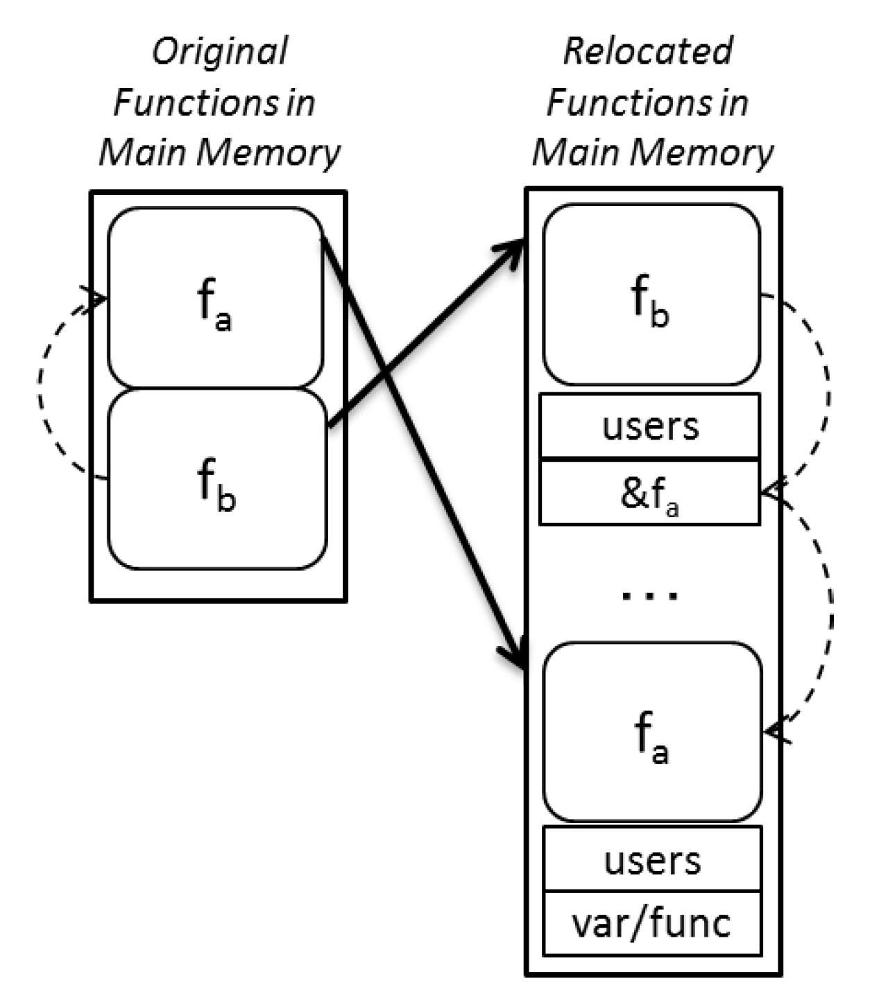
2.1. Memory-Placement Software Randomization

This set of techniques, which we refer to as SWrand for short, aims at exploring arbitrary memory placements, which ultimately determine cache behavior for both, code and data. The randomization of the memory placement can alter the hit/miss behavior and the possible contention experienced in the access to shared resources—when accessed by other applications or other threads of same application; and thus, it can affect the execution time of the application under study. SWrand builds upon the idea that, given a cache memory with S cache sets, two addressable data (e.g., double-words) belonging to objects (e.g., function code) randomized independently, have a probability of them being mapped in the same set, and thus compete for the cache space in one set, which may lead to potential cache misses due to mutual evictions. Such probability can be approximated as follows, where $P_{same-set}\left(2\right)$ stands for the probability of the two data being randomly placed in the same set:

$$P_{same-set}\left(2\right)=\frac{1}{S}.$$

(1)

Thus, upon the access of a sufficiently large number of independently randomized data (N data), the probability of all of them being mapped to the same set, which would lead to the worst potential conflicts, would be approximated as:

$$P_{same-set}\left(N\right)=P_{same-set}(N-1)·\frac{1}{S}=\frac{1}{S^{N-1}},$$

(2)

where $N>2$. Thus, there is a decreasing probability of worst-case conflicts as N increases. Instead, in a non-randomized system, unless those data can be proven to be mapped to different cache sets, the worst-case conflicts must be assumed true since they could occur systematically.

There are different incarnations of SWrand, depending on whether randomization is introduced dynamically in the different runs of a single binary, or whether memory placement is performed statically at compile-time (and thus; we need to generate multiple instances of the binary each one with a different random placement). The latter, often known as static SWrand [20,21], randomizes the location of the different objects at run-time, thus removing any type of indirection during execution, or code copy to different memory locations, which is against some basic principles for critical real-time embedded systems. In our context, HPC systems are not subject to the same set of strict constraints as critical real-time embedded systems since they do not have to undergo any strict functional safety certification and hence, the most flexible incarnation of SWrand—dynamic SWrand [16,17]—can be used instead. Such dynamic SWrand is the approach we detail next, emphasizing how it fits the proposed methodology.

2.2. Code Randomization

SWrand copies functions’ code at random memory locations during execution with the objective of randomizing their cache placement and hence, how code conflicts in first level (L1) instruction caches with OS code, dynamic libraries and other applications, and additionally with data in caches shared amongst code and data. This is illustrated with the scheme in Figure 1. The plot in the left shows how functions $f_a$ and $f_b$ are allocated in memory without SWrand, and $f_b$ calls $f_a$. On the right, we observe how functions are randomly placed in memory and function calls replaced by indirect calls whose pointers in the caller are replaced with the newly allocated location of the callee. We refer the interested reader to the original publication for further details [17].

There are two main ways to perform code randomization—at initialization or at call time [22]. The former performs the copy of all functions to random locations and the arrangement of all pointers for indirect calls before starting the execution of the code in the main function. This incurs in some overhead to copy those functions that will never be called. To mitigate this overhead, the latter approach performs a lazy allocation so that pointers for indirect calls are not set at initialization and, instead, every time a function is called, it is checked whether the pointer has already been initialized. If this is the case, then the function has already been called before. Otherwise, it is the first function invocation and hence, the code is copied into a random location opportunistically and the pointer is set accordingly.

Note that in both cases, some memory is allocated from the heap in a random location to copy the code in it. Such random location is not selected across the whole memory space for the sake of efficiency and, instead, it is limited to an offset of, at most, the size of one cache way of the largest cache in the system. Within such region, random placement is performed. Note that using a random allocation across a larger space does not bring further benefits since the sets where code is effectively placed in cache are obtained with the address modulo the size of the cache way.

In order to use this technique in the context of HPC applications, which may be potentially multi-threaded, we note that opportunistic allocation at call time cannot be used since one thread will set a pointer on a function call (in local memory space). Consequently, this specific memory address may not be visible by the other threads or may bring inconsistency problems needed for explicit synchronization. Instead, if code randomization is performed at initialization time before threads are spawned, we eliminate this problem by construction.

Observation 1.

Code randomization must be applied at initialization time for HPC systems.

Since code randomization is applied once for all functions (at initialization time), its complexity in terms of times that randomization occurs is $O\left(N_{functions}\right)$, where $N_{functions}$ stands for the number of functions in the code. Instead, in terms of memory copied, since all code of all functions needs to be copied somewhere, complexity would be expressed as $O\left(size\right(code\left)\right)$, where $size\left(\right)$ is a function of the bytes (e.g., bytes, words, double-words) of its parameter.

2.3. Stack Randomization

Dynamic stack randomization builds upon placing the function stack at a random location for each function. This can be done using indirections and allocating the stack from the heap, as in the case of code [17]. In particular, the solution builds upon having a pool of preallocated stack frames that are given to the functions called on demand. However, in the context of HPC applications, which may run multiple threads simultaneously, managing a pool of stack frames imposes the use of synchronization primitives and may decrease performance due to sharing such pool.

Static SWrand [20,21], instead, builds upon inserting padding (e.g a random size -but constant for each binary produced dummy variable) at the beginning of the stack frame so that the location of the data used from the stack is effectively random. While such a solution imposes a fixed stack frame location for each function, and thus not random across calls, we use a dynamic variant of it, where the padding created is sized randomly on each invocation locally for each function, again limited to the size of the largest cache way in the system. Since data is kept in the local stack frame of the thread, no synchronization is needed across threads.

Observation 2.

Stack randomization must be applied independently for each thread with a random shift of the stack on a function invocation for HPC systems.

Since stack randomization is applied once per function call, its complexity in terms of times that randomization occurs is $O\left(N_{calls}\right)$, where $N_{calls}$ stands for the number of function calls occurring during program execution.

2.4. Heap Randomization

SWrand, by default, does not consider heap randomization per se since, critical real-time embedded systems are not allowed to allocate memory dynamically. Hence, specific randomization for heap objects is not needed as a goal. However, SWrand builds upon random heap object allocation provided by Stabilizer [16], a compiler pass developed within the LLVM compiler and a runtime system based on Die-Hard [23] and Heap-Layers [24] providing random allocation of objects.

In the case of HPC applications, dynamic memory allocation is allowed. Building upon a centralized memory allocator for the heap imposes the use of synchronization. Whether such memory allocator is randomized or not is irrelevant in this respect and hence, SWrand does not bring any additional constraint and can be used for HPC applications regardless of whether they are single- or multi-threaded.

Observation 3.

Heap randomization does not impose any additional constraint for HPC applications.

Since heap randomization is applied upon memory allocation, with a random memory allocator layer sitting in between program calls to it and the system memory allocator, its complexity in terms of times that randomization occurs is $O\left(N_{mallocs}\right)$, where $N_{mallocs}$ stands for the number of times memory is allocated during program execution.

2.5. Summary

Overall, SWrand can be used for HPC applications, even if they are multi-threaded. However, specific considerations need to be taken into account for code and stack randomization, as detailed above. Once those considerations are taken into account, SWrand provides means to test any cache placement probabilistically, which calls for appropriate probabilistic means to analyze execution times obtained with SWrand-based test campaigns.

Note, however, that SWrand builds on the assumption that random choices related to the placement of objects are truly random. This is ensured by guaranteeing the use of an appropriate Pseudo-Random Number Generator (PRNG). In the context of our work, since we use SWrand, virtually any PRNG can be used because it does not have to be implemented in hardware, and even the default one in the standard C library meets the requirements for a PRNG in terms of degree of randomness and sufficiently long cycle before repeating. In any case, we could build upon a PRNG based on a linear-feedback shift register [25] if needed, which has been proven to comply even with the strict requirements of safety-critical systems and to have low implementation costs. Overall, random parameters used for each randomization type can be guaranteed to be truly random and thus, cause no specific bias that could challenge the quality of the results otherwise.

The next section reviews an MBPTA method, as needed to analyze randomly sample execution time measurements, making considerations for its reliable use in the context of HPC applications.

3. Measurement-Based Probabilistic Timing Analysis for HPC

A number of methods have been proposed for MBPTA [11]. Amongst those, MBPTA-CV [15] offers a detailed explanation of its implementation details as well as a publicly available implementation [26]. Therefore, we consider MBPTA-CV as the basis of our work. In this section, we review its main steps and assess their applicability in the context of HPC applications.

3.1. MBPTA-CV Fundamentals

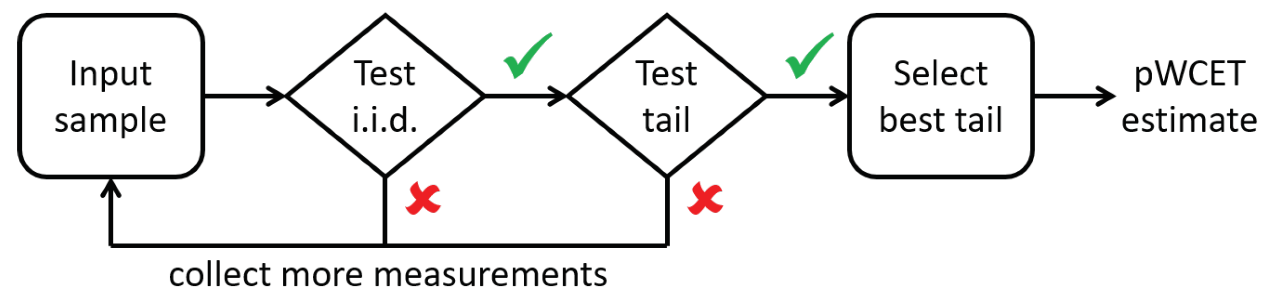
MBPTA in general, and MBPTA-CV in particular, builds upon Extreme Value Theory (EVT) [27,28], a branch of Statistics aiming at predicting rare events beyond those observed in an input sample. In the context of MBPTA, EVT is used to deliver a probabilistic WCET (pWCET) or, in other words, a distribution for high execution times so that the pWCET curve can be used to determine the probability of exceeding any particular execution time. Such pWCET curve is normally depicted as a Complementary Cumulative Distribution Function (CCDF), as the example shown in Figure 2, where the red dotted line corresponds to a sample of 1000 execution time measurements and the black straight line the pWCET curve. The y-axis corresponds to the exceedance probability (in logarithmic scale), and the x-axis shows execution time in seconds. For instance, we observe that the probability of exceeding an execution time of 7.4 s is up to ${10}^{-12}$ per run.

MBPTA-CV builds upon Generalized Pareto Distributions (GPD) for tail modelling, whose Cumulative Distribution Function (CDF) can be expressed as follows:

$$H(x;\mu ,\sigma ,\xi )=1-{\left[1+\xi \left(\frac{x-\mu }{\sigma }\right)\right]}^{-1/\xi },$$

(3)

where the parameters $\mu$, $\sigma$ and $\xi$ are known as the location, scale and shape respectively. In particular, the authors of Reference [15] show that reliable and tight pWCET estimates can be obtained restricting $\xi =0$ based on the fact that execution time of finite programs is finite, which excludes heavy tail models (i.e., $\xi >0$), and on the fact that, among the remaining cases (i.e., $\xi \le 0$), $\xi =0$ (exponential tail) upper bounds all of them.

MBPTA-CV uses the residual coefficient of variation (residual $CV$), where the $CV$ for a given distribution is obtained as the ratio between its standard deviation and its mean. The (theoretical) residual $CV$, for a given threshold $th$, referred to as $C{V}_{theo}\left(th\right)$ is obtained as follows:

$$C{V}_{theo}\left(th\right)=\frac{\sqrt{V\left(th\right)}}{M\left(th\right)},$$

(4)

where, for a given threshold value $th$, $M\left(th\right)$ is the mean of the excesses (values above $th$ subtracting $th$ to each one), and $V\left(th\right)$ their variance.

The residual $CV$ has been shown to determine the type of the tail of the distribution: $CV=1$ for exponential tails, $CV\ge 1$ for heavy tails and $CV\le 1$ for light tails [29]. As discussed before, the only reliable type of tails applicable to any program with finite execution time generally corresponds to exponential tails.

Such residual $CV$ can be estimated with the empirical residual CV using the observed mean and standard deviation from a sample rather than theoretical parameters, and used to produce the CV-plot, which estimates the $CV$ for each number of exceedances of a sample. Using the observed mean and standard deviation of the sample, namely $\overline{x}$ and $sd$ respectively, leads to the following expression for the $CV$:

$$CV\left(th\right)=\frac{sd}{\overline{x}}.$$

(5)

An example of a CV-plot is shown in Figure 3. The x-axis shows, for a sample of 1000 measurements, out of which the 500 lowest values are discarded, from left to right the number of exceedances discarded. For instance, when the x-axis indicates 400, it indicates that only the highest 100 values of the sample are retained, and the blue line indicates the estimated $CV$ for those exceedances. The red lines include the range of values where the exponentiality assumption for the tail cannot be rejected with 95% confidence. If the blue line is below both red lines, then exponentiality is rejected and the tail is regarded as light. Hence, in this case using exponential tails is pessimistic but reliable for pWCET estimation. However, if the blue line is above both red lines, then exponentiality is rejected and the tail is regarded as heavy, thus meaning that exponential tails cannot be used. In the case of MBPTA-CV, the CV-plot is used to guarantee that the set of highest values used for pWCET estimation can be approximated with an exponential tail reliably.

3.2. MBPTA-CV Steps

Next, we review the steps of the MBPTA-CV process and assess their fit for HPC applications on HPC systems. Figure 4 depicts the steps needed from the input sample collection to the computation of a valid pWCET estimate. Next subsections, describe each one of the steps involved.

Input Sample Generation

MBPTA-CV application process starts with the collection of an execution time sample. In the default application of the method, such sample must have at least 100 execution time measurements, although, in general, the larger the sample, the higher the chances to converge and deliver a pWCET estimate. Moreover, in general, larger samples have more information about the distribution and hence, pWCET estimates obtained will be tighter.

Depending on the duration of the HPC application under analysis and the computing resources available, the number of measurements that may be collected may vary. We note that MBPTA-CV requires 100 measurements because the lowest half is discarded considering that they are not appropriate to predict high execution times, and at least 50 measurements (maxima) are needed to derive a highly reliable pWCET estimate, as needed for critical real-time embedded systems. However, as noted by the authors of Reference [15], different applications of EVT allow the minimum number of maxima used to fit a tail to be between 10 and 50. Therefore, we note that, although the reliability and tightness of the pWCET distribution may decrease, using samples of only 20 measurements is still possible—with the lowest half being discarded—while having a sound application on MBPTA-CV. Note that, in this case, the 10 maxima should allow fitting a tail reliably. Otherwise, a larger sample would be needed until having at least 10 maxima allowing such reliable tail fitting.

Observation 4.

The lowest number of execution time measurements to use MBPTA-CV for HPC applications can be decreased down to 20, instead of 100.

3.3. Independence and Identical Distribution

Input data must be independent and follow an identical distribution (i.i.d.), which, in practice, means that execution time measurements have been collected with the same initial conditions. For instance, this is achieved by collecting execution times for the HPC application on the same system resetting any state remaining from previous executions before each experiment, and using either the same input set or choosing the input set randomly out of a pool of relevant input sets.

In the context of HPC systems, while we can control input data and some state for the application under analysis, some other activities (e.g., periodic OS services) may not be sufficiently controlled and may affect differently each execution measurement. Moreover, such impact may be periodic, so that i.i.d. properties across measurements do not hold. However, as shown in Reference [30], i.i.d. properties do not need to hold for all measurements but only for maxima (i.e., the subset of measurements above a given threshold used to draw the tail with EVT). This, in essence, implies that the impact of those OS services must have a sufficiently low relative impact not to make non-maxima become maxima. In general, OS services may take up to few milliseconds to execute. Hence, by analyzing applications whose execution time is some orders of magnitude higher (e.g., hundreds of milliseconds or more), the impact of OS noise becomes irrelevant in practice. Still, i.i.d. properties of maxima need to be statistically tested for a reliable application of EVT as part of MBPTA-CV.

Observation 5.

I.i.d. properties may not hold for HPC applications, but, as long as execution time is large enough, i.i.d holds for maxima, which is enough for a reliable application of MBPTA-CV.

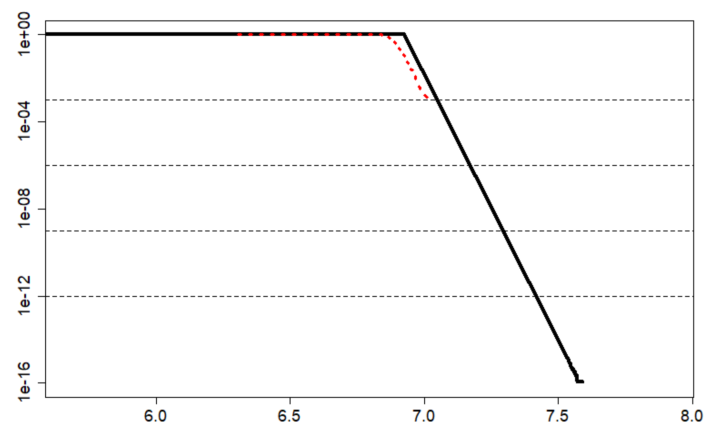
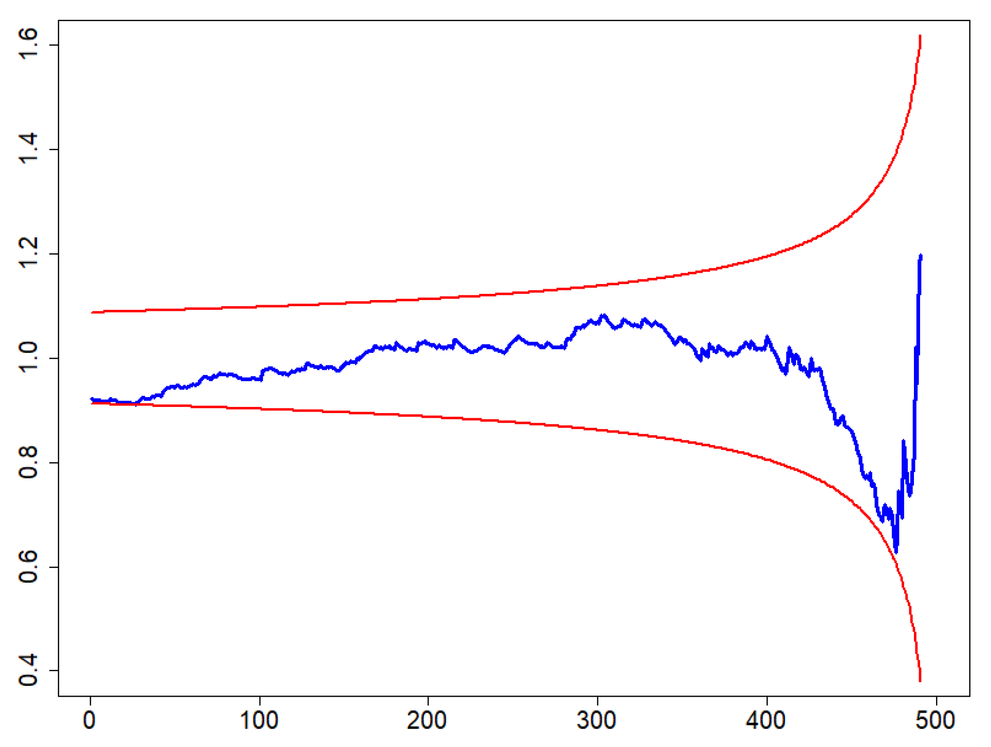
3.3.1. Exponential Tail Test

MBPTA-CV, as explained before, builds upon the CV-plot to test whether the maxima retained for pWCET estimation are compatible with the exponential assumption. In other words, such maxima is regarded as acceptable if maxima are either compatible with exponential or light tails, since both are reliably upper-bounded with exponential tails. If maxima in the sample fails to fulfill such statistical criteria, since the distribution under analysis must meet this probabilistic property by construction, a larger sample is requested until, eventually, it converges.

The particular method considered, MBPTA-CV, in fact, imposes that not only those maxima used for pWCET estimation must be compatible with the exponential assumption, but also smaller sets of maxima with at least 10 measurements (based on common practice, smaller sets of maxima are regarded as unreliable [15].). Since MBPTA-CV imposes the use of at least 50 maxima, then all sets of maxima between 10 and 50 elements must pass the exponentiality test (i.e., have the $CV$ estimator below the top red line for all those sets of maxima). As discussed for the sample generation, fitting the tail with only 10 maxima, while less reliable, it is still acceptable based on common practice. Hence, the exponentiality test provided by the CV-plot is also restricted to such set of maxima, which facilitates passing it.

Observation 6.

The exponential test may be less demanding for HPC applications if the smallest set of maxima to estimate the pWCET distribution is decreased below 50 measurements (being at least 10).

3.3.2. Select the Best Tail

Once there is at least a set of maxima passing the exponentiality test, selecting the best set of maxima is an arbitrary choice statistically speaking since any set is equally statistically valid, as pointed out in Reference [15]. In the case of MBPTA-CV, out of all sets of maxima passing the test, the one with a $CV$ estimator closer to 1 (the expected value for exponential tails) is used. In the case of HPC applications, there is no particular reason to change this criteria.

Observation 7.

The criteria to select the best tail remains unchanged for HPC applications.

3.3.3. pWCET Estimate

Once determined the set of maxima to use for pWCET estimation, fitting an exponential tail is an automatic step independent of any other consideration, such as, for instance, the application under analysis or the domain of such application. However, the particular exceedance probability to consider may change across domains. In the case of critical real-time embedded systems, such probability normally relates to acceptable failure rates or residual risk as determined in the particular functional safety standard in the domain.

In the case of HPC applications, in general, no such standard exists. In general, those applications, rather than safety critical, are mission critical, thus meaning that a failure to execute properly diminishes the success of the mission. For instance, acceptable failure probabilities for safety-critical systems may be in the order of ${10}^{-12}$ per run, whereas an HPC application processing, for instance, soil data to detect appropriate locations to set oil wells may afford higher failure probabilities (e.g., ${10}^{-6}$ per run).

Observation 8.

Exceedance probabilities acceptable for HPC applications may differ from those usually considered for critical real-time embedded systems.

3.4. Summary

As described in this section, the use of MBPTA-CV in the context of HPC applications is viable as long as particular considerations are taken into account. Those considerations relate to choosing appropriate sample sizes, with less demanding criteria than for critical real-time embedded systems, and appropriate measurement collection protocols to achieve i.i.d. at least for maxima. Constraints for exponentiality compliance can also be decreased, and acceptable exceedance probabilities may be, in general, higher than those for critical real-time embedded systems.

Regarding complexity, since i.i.d. tests are applied only over the maxima, their complexity is limited by the number of maxima retained. Such maxima are, in turn, limited by the exponential tail test, the implementation of which in Reference [26] is limited to a fixed maximum number of maxima (e.g., 10,000 measurements). Thus, only a subset of maxima is retained, thus limiting the cost of the exponential tail test, the i.i.d. tests, and any step thereafter for tail selection and pWCET estimation. However, in order to retain that number of maxima, the full execution time sample needs to be sorted first, thus being the cost of the overall process of $O(RlogR)$, where R stands for the number of application runs (execution time measurements).

4. Evaluation

This section presents the case study used for the evaluation of the proposed approach, describes the experimental framework, and provides a set of results validating the approach.

4.1. Case study

The case study considered in this paper is the Full Waveform Inversion (FWI), a cutting edge technique that aims to acquire the physical properties of the subsoil from a set of seismic measurements [18,19]. Starting from a guess (initial model) of the variables being inverted (e.g., sound transmission velocity), the stimulus introduced and the recorded signals, FWI performs several phases of iterative computations to reach the real value of the set of variables being inverted with an acceptable error threshold. From a purely computational point of view, the reason why this application is very suited for an HPC system is that the initial field is split among a huge number of disjoint datasets, which can be processed independently. Once a set of signal sources and receivers has been selected, the field can be decomposed, and later on computed using traditional means (e.g., OpenMP, CUDA, MPI, …). This makes this problem an embarrassingly parallel one. FWI consists of multiple phases, grouped into these:

• Pre-processing: data is read from disk and several checks are performed to ensure that the subsequent processing is valid.
• Main processing: composed essentially by a frequency loop, the goal of this phase is to iteratively obtain the real value of a given variable (or a set of variables) from an initial guess. To do this, the signal of the input sources and the received data is bandpass-filtered to the frequency of interest by means of an adjoint-state method. The input model is modified to that with the smallest error. Once this has been achieved, another frequency is considered.
• Post-processing: the objective of this phase is to ensure that the numerical values of the generated output are quantitatively correct. Also, it holds all the specific routines to adapt the data to the output expected by the user (interpolation, file formats, etc.).

The computing kernel of this application is an iterative 4th order 3D stencil process, where each element of the data matrix is obtained as a function of 13 points that include 12 neighbor points and the own data point being estimated. Thus, on each iteration of the algorithm, all points of the 3D data matrix are updated converging to a precise representation of the specific variable being modelled. Figure 5 illustrates the specific points used for the computation of each point in each iteration, which include the two closest points in each direction of the 3 dimensions, as well as the point being updated.

4.2. Experimental Framework

In order to evaluate the FWI case study, we have used as representative HPC system an Intel platform. Such platform includes two sockets with an Intel Xeon Platinum 8160 24-core at 2.1 GHz with 96 GB of DDR4-2667 memory shared between the sockets (2 GB per core). For the sake of restricting the study to an homogeneous platform where scalability can be understood without disruptions caused by intra/inter-socket variations, we restrict our evaluation to a single socket. In that case, we consider different thread counts when parallelizing the kernel of the application with OpenMP: 1, 2, 4, 8, 12 and 24 threads. The OS used by this platform is SUSE Linux Enterprise Server 12 SP2.

Regarding the use case, the 3D input data matrix must be sized conveniently to meet two requirements:

• Be representative of real problems.
• Deliver execution times no less than hundreds of milliseconds, as explained before, for a reliable application of MBPTA-CV despite OS noise.

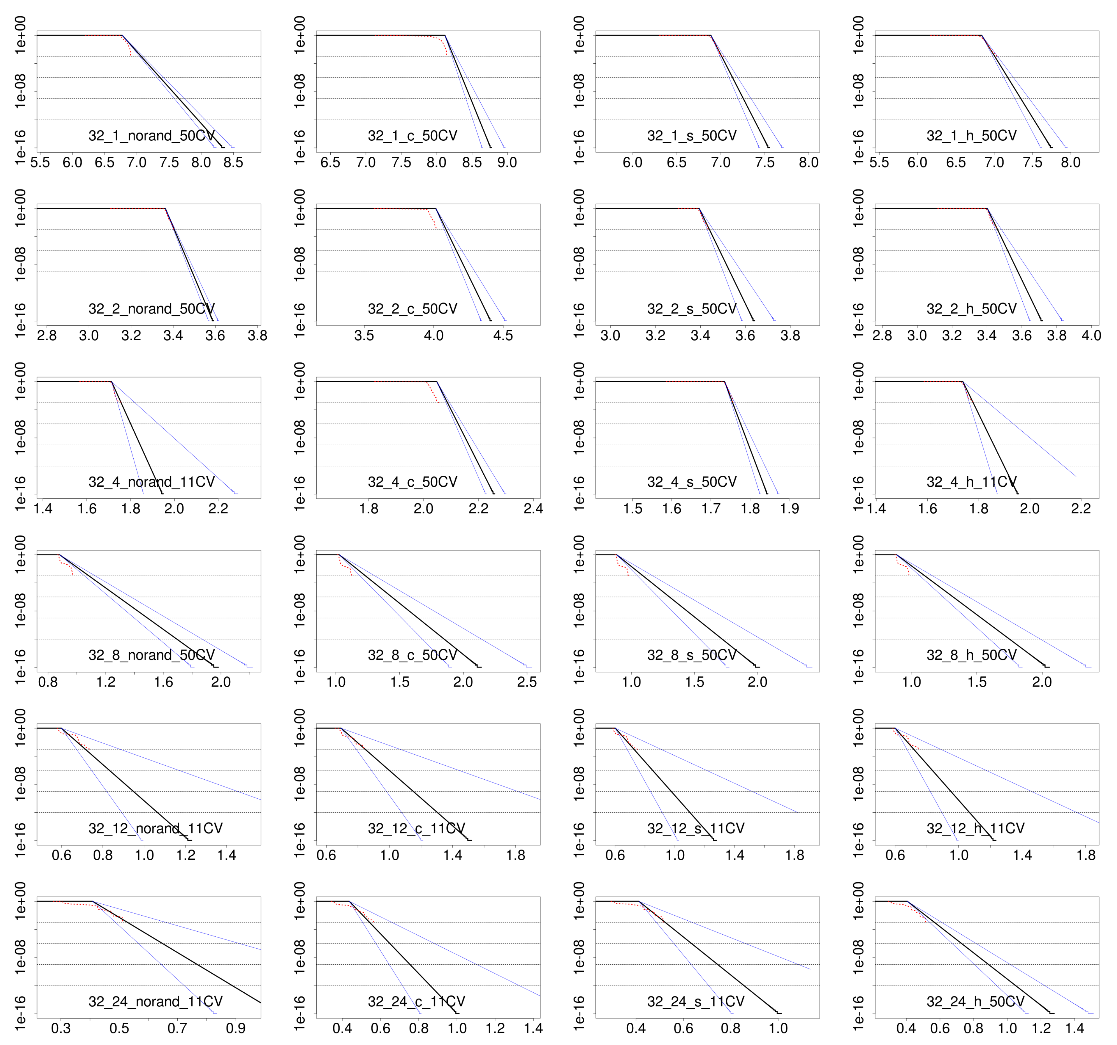
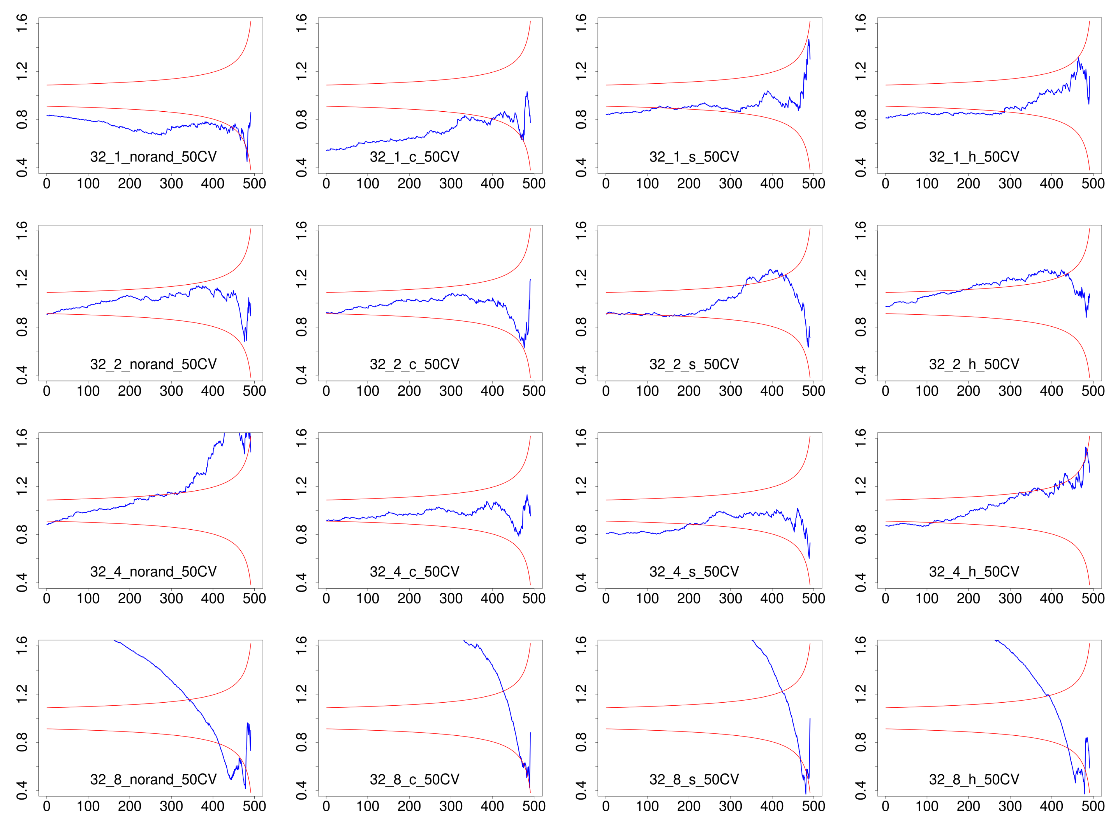
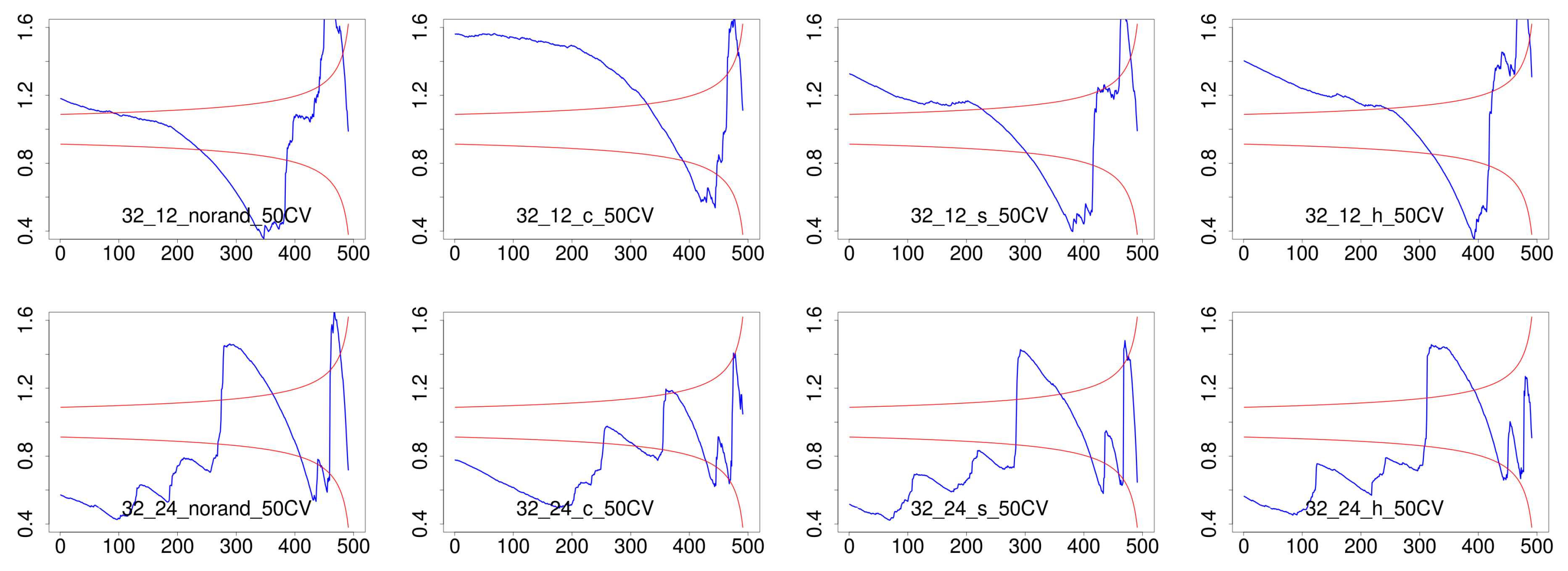
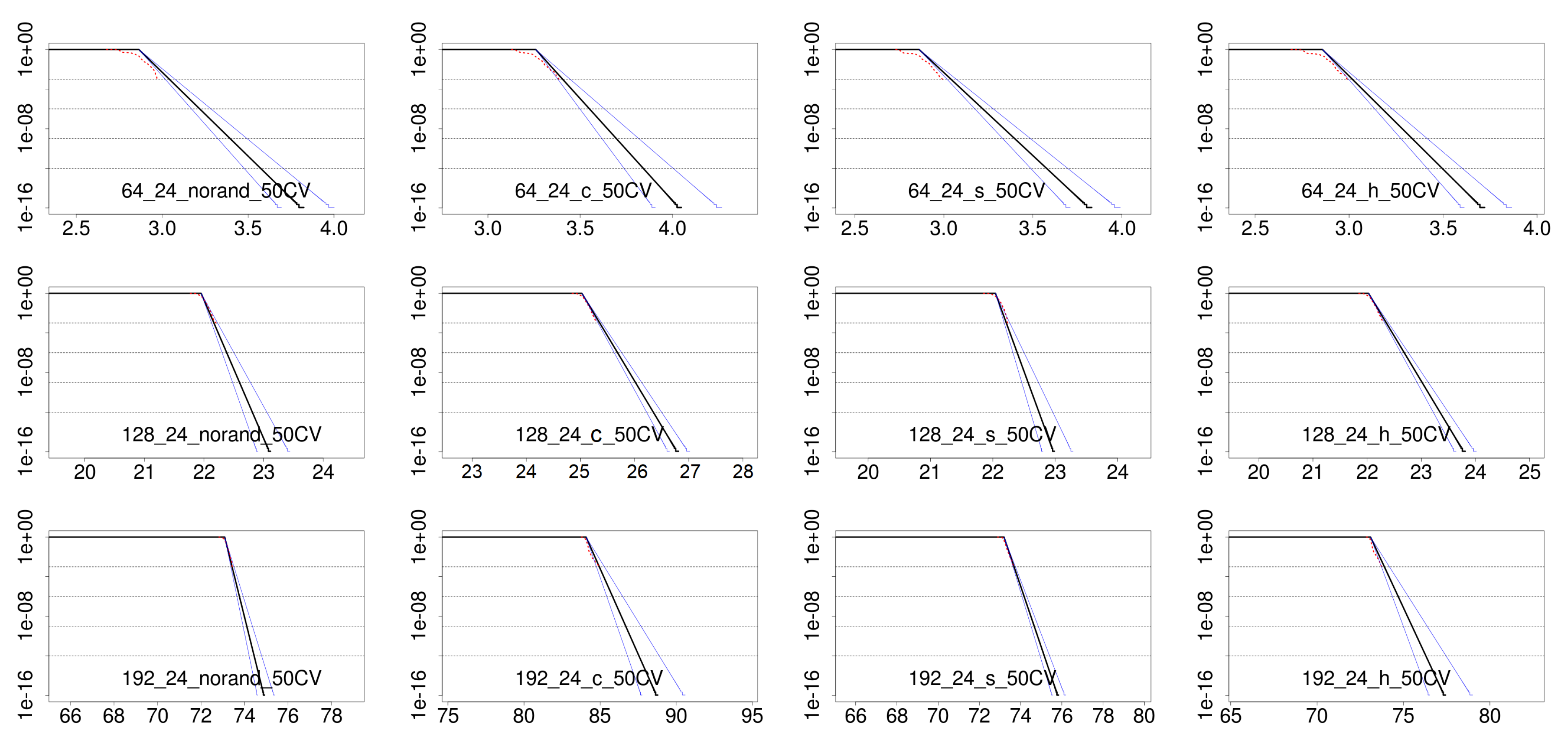
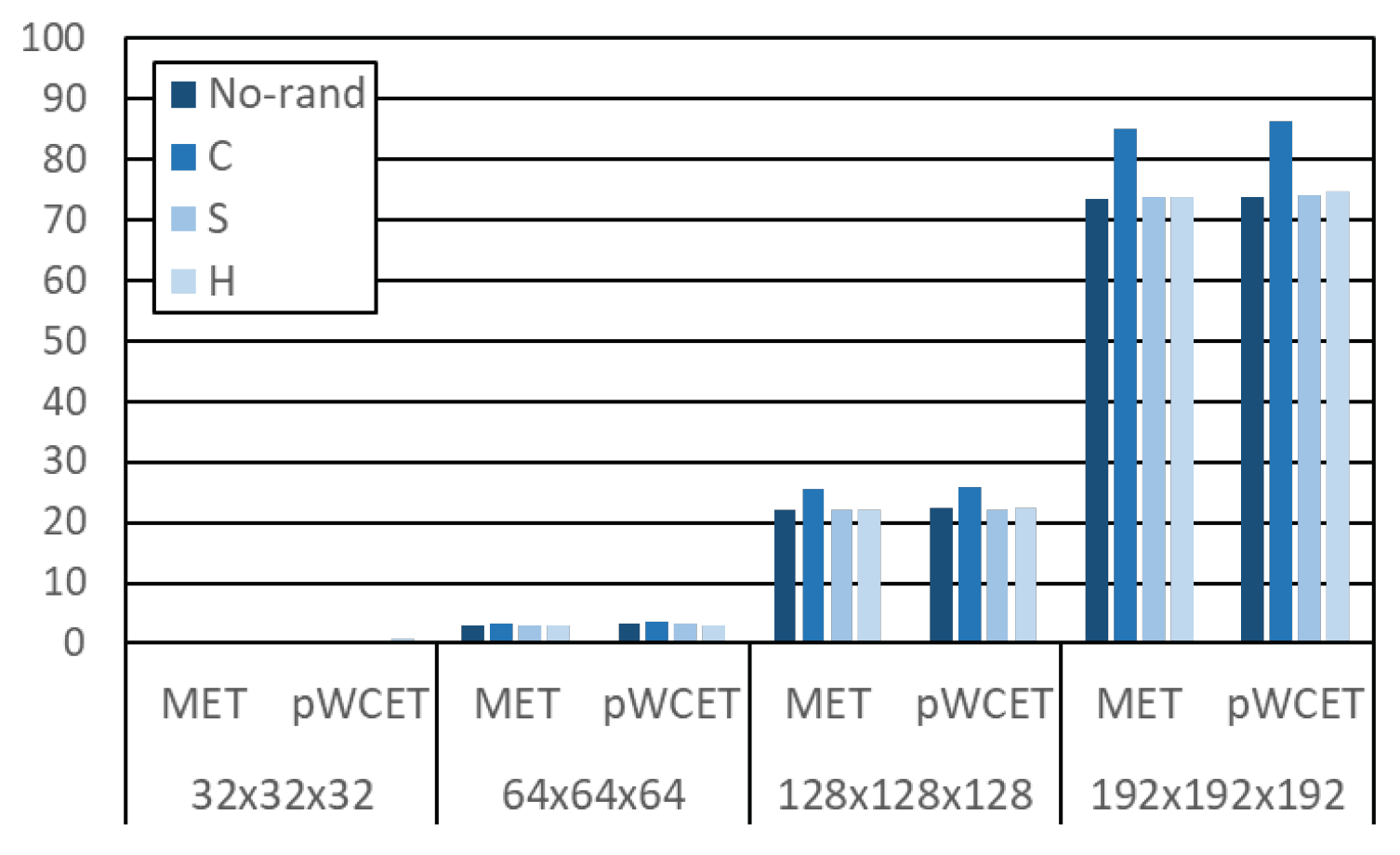
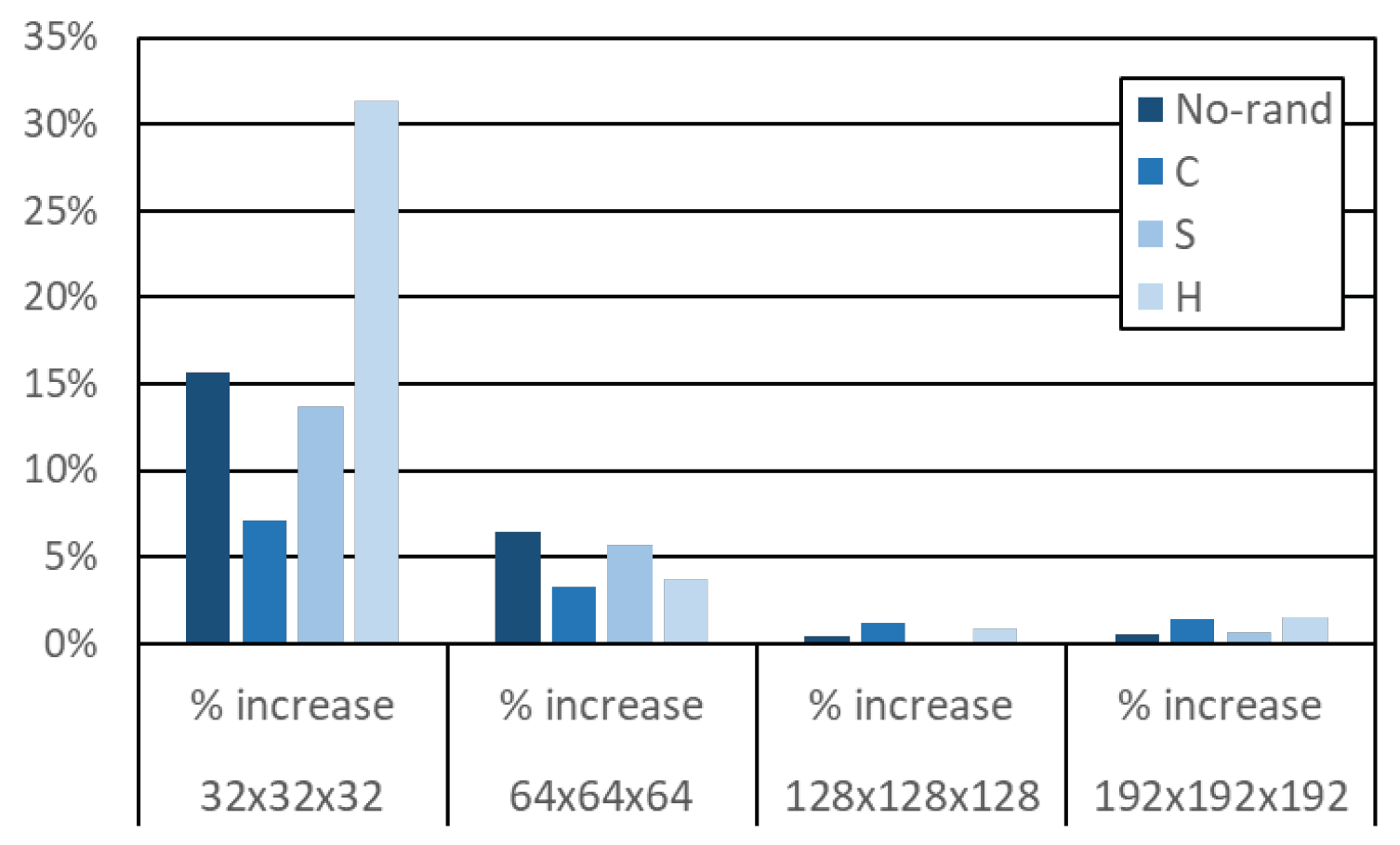
For that purpose, matrix sizes of N elements in each dimension have been considered, being N 32, 64, 128 and 192 (e.g., 32 × 32 × 32 and so on and so forth). All thread configurations have been studied for $N=32$ and $N=64$. However, due to the computation cost of larger matrices, we only consider the case with 24 threads for $N=128$ and $N=192$.

We have integrated the FWI application with the Stabilizer library to apply SWrand as detailed in Reference [17]. This allows each application run to exercise different random values, which lead to random placements for those features for which randomization is enabled (namely code, heap or stack). Each configuration of a given matrix size and thread count has been run 1000 times, thus making sure that enough measurements are available to MBPTA-CV. We have followed all steps of MBPTA-CV, thus passing first all i.i.d. tests. This is fully expected for randomized setups. In the case of the non-randomized executions, platform noise (OS, initial state, etc.) has turned out to be sufficient to provide those properties statistically, despite they may not necessarily hold by construction. The suitability to obtain pWCET estimates with MBPTA-CV has been assessed with the CV tests of MBPTA-CV and, in all cases, have been passed as discussed in more detail later. Then, once all tests have been passed, we have obtained the pWCET estimates for all scenarios considered, which includes, apart from different matrix sizes, also different thread counts. We build our discussion hereafter building on those measurements, which allowed for a smooth application of MBPTA-CV once all the cautionary measures in the process (namely, the observations made in this paper) have been taken into account.

4.3. Results

Figure 6 shows the pWCET distributions for the FWI case study with a problem size of 32 elements in each dimension, for 1, 2, 4, 8, 12 and 24 threads from top to bottom, and for no randomization, code randomization, stack randomization and heap randomization from left to right. Note that actual measurements for no randomization (red dotted lines in “norand” plots) correspond to actual measurements in the default platform, thus representative of MBTA practice on top of which an engineering margin should be added to account for the unknown. Since such a margin is extremely hard to determine, particularly for multicores [8], we have applied MBPTA-CV on top of those measurements (pWCET distributions for “norand” plots) to have a form of informed engineering margin on top of which we can reason.

The key insight of these results is the ability of software randomization to effectively work on HPC applications and systems, and the ability of MBPTA to estimate pWCET distributions for HPC applications and systems. We also note that, as we increase the number of threads, both, the execution time distribution and the pWCET distribution decrease quite in line with the number of threads, thus obtaining 2× and 4× speedups with 2 and 4 threads respectively w.r.t. the single-threaded case. However, further increasing the threads produces diminishing returns with much lower relative speedups. Across the different types of randomizations, we observe that heap and stack randomization cause little overhead w.r.t. the non-randomization case. However, the slowdown for code randomization is more significant, typically around 20%.

Another relevant observation is the fact that execution time variability, in absolute terms, remains quite stable, with a tail variability in the order of 100 ms. This is shown in the red dotted lines in the plots, where we see that the distance in the x-axis between the point at which the tail starts to fall until the point the tail of the observed sample ends spans around 0.1 s (100 ms). Such variability, caused inevitably by the combination of the initial state of the platform when the application is run, the OS noise, DRAM refresh, and any other uncontrolled source of jitter in HPC platforms, has an impact in the pWCET distributions. In particular, it impacts tail fitting making the tail slope account for such variability. Most of the cases, such 100 ms variability in the tail observations leads to a 500 ms variability between the pWCET values at probabilities $1.0$ and ${10}^{-12}$ (0.5 s in the plots). Visually, this leads to sharp slopes for low thread counts, since the relative impact of this variability is low w.r.t. the absolute pWCET values. However, increasing thread counts make such relative impact larger, thus leading to softer slopes visually, although the slope, in general, remains highly stable in absolute terms. Note that, in general, those sources of execution time noise are mastered (e.g., resetting initial state, using less intrusive OS services, etc.), at least to some extent, in embedded real-time systems, thus being such relatively high amount of noise a particular characteristic of HPC systems.

Together with pWCET estimates, we have obtained the CV-plot for each configuration as shown in Figure 7. For instance, the case for no randomization and 4 threads (third plot in first row) and no randomization and 12 threads (fifth plot in first row), have CV values in the region of heavy tails for 50 maxima (above the two red lines). However, when considering only 10 maxima, then the CV values are within the exponential range. Thus, for these two cases we obtained the pWCET distributions in Figure 6 imposing the use of at least 10 maxima instead of imposing the use of 50 maxima. In fact, out of the 24 cases in the figure, 9 of them where obtained with a limit of at least 10 maxima rather than at least 50, thus emphasizing the importance of relaxing this constraint for HPC systems.

Analogous results have been obtained for other problem sizes, as shown in Figure 8. Problem sizes of 64 × 64 × 64, 128 × 128 × 128 and 192 × 192 × 192 are shown from top to bottom, for no randomization, code randomization, stack randomization and heap randomization from left to right. The corresponding CV-plots are also shown in Figure 9 for the sake of completeness. As shown, pWCET distributions accurately model tail distributions for high execution times. In these cases, at least 50 maxima could be used in all configurations. As before, code randomization introduces larger overheads than other types of randomizations, being in this case in the range 10–20% typically.

Note that, while the pWCET distribution and CV-plot across randomization types are essentially similar, SWrand provides guarantees on the fact that code, stack and heap allocation cannot create unexpected execution time disturbances, because it reduces the risk that all of them result in a pathological memory layout.

Finally, we show the absolute maximum execution time (MET) and pWCET estimates at an exceedance threshold of ${10}^{-6}$ per run in Figure 10. As shown, absolute differences are small, thus showing that pWCET estimates are very close to the MET out of 1000 runs in absolute terms, which indicates that unobserved execution times can only be slightly higher than observed ones. Moreover, results show that stack and heap randomization cause little performance variation. However, code randomization causes a noticeable impact in MET and pWCET estimates, thus showing that code memory placement is particularly critical for this application. Relative results on the increase of the pWCET estimates w.r.t. MET are shown in Figure 11. As we increase problem size, execution time variability decreases in relative terms, which leads to sharper pWCET distributions and hence, smaller increase in relative terms of the pWCET estimates w.r.t. MET. Hence, the larger the problem size is, the more stable the execution time is. The use of SWrand along with MBPTA-CV provides strong guarantees on these observations, thus allowing an efficient use of resources scheduling HPC applications accounting for their unobserved high execution times.

5. Related Work

The statistical analysis of complex systems is a popular cross-domain approach due to the system-agnostic nature of statistics, which allows using them virtually in any domain—as long as they are properly applied. This includes neural networks, Bayesian models and fuzzy logic (the latter not being strictly about statistics) among others applied to domains such as robotics, medical, and character/numeral recognition, to name a few [31,32,33,34].

In the context of timing analysis—the focus of our work, the critical real-time embedded systems domain is prolific in techniques for WCET estimation. A family of techniques is based on the static analysis and abstract interpretation of the software under analysis on a timing model of the hardware platform [7]. However, it has been shown that those methods are appropriate for very simple microcontrollers [8], far simpler than those in HPC systems.

On the other side of the spectrum, we can find measurement-based timing analysis techniques, which have been used in many real systems due to their flexibility and portability to virtually any platform [6]. Most of those techniques aim at estimating a deterministic WCET estimate that must hold under any circumstance, which often leads to a tradeoff between reliability and tightness. In general, those approaches build upon collecting execution time measurements and adding an engineering margin on top of the maximum observed execution time, whose reliability is hard—if at all possible—to assess [8].

Still in the area of measurement-based timing analysis techniques, a new family of techniques has been proposed, building on probabilistic principles to derive a pWCET rather than an absolute bound [11]. Those techniques build upon appropriate measurement collection protocols as well as, potentially, on specific platform support—either hardware or software—to increase the representativeness of the tests used for pWCET estimation. Amongst those techniques, in this work we focus on MBPTA-CV [15], since a detailed method description and an actual implementation are publicly available.

Most MBPTA methods build upon the assumption of independent data or, at least, independent maxima. However, some works have shown that some weak dependence can also be acceptable [27,35].

Finally, to the best of our knowledge, no specific methods have been devised to predict reliably high execution times of HPC applications. Hence, our adaptation of a mechanism—MBPTA-CV—used in another domain to fit the needs and constraints of HPC systems is a pioneering attempt to reach the goal of reliable and tight estimation of execution time bounds for HPC applications.

6. Conclusions

The availability of HPC platforms nowadays has led to a plethora of HPC applications in a variety of domains and contexts. Such ubiquity of HPC has made a number of new requirements emerge. Out of those, timing guarantees are particularly important for a number of applications with real-time needs.

This paper shows how some techniques based on software randomization and MBPTA, if used reliably, allow performing extensive and representative execution time test campaigns for HPC applications and predicting high execution times. Our results on a parallel application used for geophysical exploration confirm our claims and show how reliable and tight pWCET bounds can be obtained for HPC applications running on HPC systems.

References

1. Agosta, G.; Fornaciari, W.; Massari, G.; Pupykina, A.; Reghenzani, F.; Zanella, M. Managing Heterogeneous Resources in HPC Systems. In Proceedings of the 9th Workshop and 7th Workshop on Parallel Programming and RunTime Management Techniques for Manycore Architectures and Design Tools and Architectures for Multicore Embedded Computing Platforms, Manchester, UK, 23 January 2018; pp. 7–12. [Google Scholar]
2. Flich, J.; Agosta, G.; Ampletzer, P.; Alonso, D.A.; Brandolese, C.; Cilardo, A.; Fornaciari, W.; Hoornenborg, Y.; Kovac, M.; Maitre, B.; et al. Enabling HPC for QoS-sensitive applications: The MANGO approach. In Proceedings of the 2016 Design, Automation Test in Europe Conference Exhibition (DATE), Dresden, Germany, 14–18 March 2016; pp. 702–707. [Google Scholar]
3. Flich, J.; Agosta, G.; Ampletzerm, P.; Alonso, D.A.; Brandolese, C.; Cappe, E.; Cilardo, A.; Dragić, L.; Dray, A.; Duspara, A.; et al. Exploring manycore architectures for next-generation HPC systems through the MANGO approach. Microprocess. Microsyst. 2018, 61, 154–170. [Google Scholar] [CrossRef]
4. Massari, G.; Pupykina, A.; Agosta, G.; Fornaciari, W. Predictive Resource Management for Next-generation High-Performance Computing Heterogeneous Platforms. In Proceedings of the 18th International Conference on Embedded Computer Systems: Architectures, Modeling, and Simulation (SAMOS’19), Samos, Greece, 7–11 July 2019. [Google Scholar]
5. Pupykina, A.; Agosta, G. Optimizing Memory Management in Deeply Heterogeneous HPC Accelerators. In Proceedings of the 2017 46th International Conference on Parallel Processing Workshops (ICPPW), Bristol, UK, 14–17 August 2017; pp. 291–300. [Google Scholar]
6. Mezzetti, E.; Vardanega, T. On the industrial fitness of wcet analysis. In Proceedings of the 11th International Workshop on Worst-Case Execution-Time Analysis, Porto, Portugal, 5 July 2011. [Google Scholar]
7. Wilhelm, R.; Engblom, J.; Ermedahl, A.; Holsti, N.; Thesing, S.; Whalley, D.; Bernat, G.; Ferdinand, C.; Heckmann, R.; Mitra, T.; et al. The worst-case execution time problem: Overview of methods and survey of tools. ACM TECS 2008, 7, 1–53. [Google Scholar] [CrossRef]
8. Abella, J.; Hernandez, C.; Quiñones, E.; Cazorla, F.J.; Conmy, P.R.; Azkarate-askasua, M.; Perez, J.; Mezzetti, E.; Vardanega, T. WCET Analysis Methods: Pitfalls and Challenges on their Trustworthiness. In Proceedings of the 10th IEEE International Symposium on Industrial Embedded Systems (SIES), Siegen, Germany, 8–10 June 2015. [Google Scholar]
9. Bernat, G.; Colin, A.; Petters, S. WCET analysis of probabilistic hard real-time systems. In Proceedings of the 23rd IEEE Real-Time Systems Symposium, Austin, TX, USA, 3–5 December 2002. [Google Scholar]
10. Cazorla, F.J.; Quiñones, E.; Vardanega, T.; Cucu, L.; Triquet, B.; Bernat, G.; Berger, E.; Abella, J.; Wartel, F.; Houston, M.; et al. PROARTIS: Probabilistically Analysable Real-Time Systems. ACM TECS 2012, 12, 1–26. [Google Scholar] [CrossRef]
11. Cazorla, F.J.; Kosmidis, L.; Mezzetti, E.; Hernandez, C.; Abella, J.; Vardanega, T. Probabilistic Worst-Case Timing Analysis: Taxonomy and Comprehensive Survey. ACM Comput. Surv. 2019, 52, 14:1–14:35. [Google Scholar] [CrossRef]
12. Kosmidis, L.; Quiñones, E.; Abella, J.; Vardanega, T.; Hernandez, C.; Gianarro, A.; Broster, I.; Cazorla, F.J. Fitting processor architectures for measurement-based probabilistic timing analysis. Microprocess. Microsyst. 2016, 47, 287–302. [Google Scholar] [CrossRef] [Green Version]
13. Milutinovic, S.; Mezzetti, E.; Abella, J.; Vardanega, T.; Cazorla, F.J. On uses of extreme value theory fit for industrial-quality WCET analysis. In Proceedings of the 2017 12th IEEE International Symposium on Industrial Embedded Systems (SIES), Toulouse, France, 14–16 June 2017. [Google Scholar]
14. Cucu-Grosjean, L.; Santinelli, L.; Houston, M.; Lo, C.; Vardanega, T.; Kosmidis, L.; Abella, J.; Mezzetti, E.; Quiñones, E.; Cazorla, F.J. Measurement-Based Probabilistic Timing Analysis for Multi-path Programs. In Proceedings of the 2012 24th Euromicro Conference on Real-Time Systems (ECRTS), Pisa, Italy, 11–13 July 2012. [Google Scholar]
15. Abella, J.; Padilla, M.; Del Castillo, J.; Cazorla, F. Measurement-Based Worst-Case Execution Time Estimation Using the Coefficient of Variation; ACM: New York, NY, USA, 2017. [Google Scholar]
16. Curtsinger, C.; Berger, E.D. STABILIZER: Statistically Sound Performance Evaluation. SIGARCH Comput. Archit. News 2013, 41, 219–228. [Google Scholar] [CrossRef]
17. Kosmidis, L.; Curtsinger, C.; Quiones, E.; Abella, J.; Berger, E.; Cazorla, F.J. Probabilistic timing analysis on conventional cache designs. In Proceedings of the 2013 Design, Automation Test in Europe Conference Exhibition (DATE), Grenoble, France, 18–22 March 2013; pp. 603–606. [Google Scholar]
18. Kormann, J.; Rodríguez, J.; Gutiérrez, N.; Ferrer, M.; Rojas, O.; De la Puente, J.; Hanzich, M.; María Cela, J. Toward an automatic full-wave inversion: Synthetic study cases. Lead. Edge 2016, 35, 1047–1052. [Google Scholar] [CrossRef] [Green Version]
19. Hanzich, M.; Kormann, J.; Gutiérrez, N.; Rodríguez, J.; De la Puente, J.; María Cela, J. Developing Full Waveform Inversion Using HPC Frameworks: BSIT. In Proceedings of the EAGE Workshop on High Performance Computing for Upstream, Chania, Crete, 7–10 September 2014. [Google Scholar]
20. Kosmidis, L.; Vargas, R.; Morales, D.; Quiñones, E.; Abella, J.; Cazorla, F.J. TASA: Toolchain Agnostic Software Randomisation for Critical Real-Time Systems. In Proceedings of the ICCAD, Austin, TX, USA, 7–10 November 2016. [Google Scholar]
21. Kosmidis, L.; Quiñones, E.; Abella, J.; Farrall, G.; Wartel, F.; Cazorla, F.J. Containing Timing-Related Certification Cost in Automotive Systems Deploying Complex Hardware. In Proceedings of the 51st Annual Design Automation Conference, San Francisco, CA, USA, 1–5 June 2014; ACM: New York, NY, USA, 2014; pp. 22:1–22:6. [Google Scholar]
22. Cros, F.; Kosmidis, L.; Wartel, F.; Morales, D.; Abella, J.; Broster, I.; Cazorla, F.J. Dynamic software randomisation: Lessons learnec from an aerospace case study. In Proceedings of the Design, Automation Test in Europe Conference Exhibition (DATE), Lausanne, Switzerland, 27–31 March 2017; pp. 103–108. [Google Scholar]
23. Berger, E.D.; Zorn, B.G. DieHard: Probabilistic memory safety for unsafe languages. In Proceedings of the ACM SIGPLAN 2006 Conference on Programming Language Design and Implementation, Ottawa, ON, Canada, 11–14 June 2006; pp. 158–168. [Google Scholar]
24. Berger, E.D.; Zorn, B.G.; McKinley, K.S. Composing High-performance Memory Allocators. ACM SIGPLAN Not. 2001, 36, 114–124. [Google Scholar] [CrossRef]
25. Agirre, I.; Azkarate-askasua, M.; Hernandez, C.; Abella, J.; Perez, J.; Vardanega, T.; Cazorla, F.J. IEC-61508 SIL 3 Compliant Pseudo-Random Number Generators for Probabilistic Timing Analysis. In Proceedings of the 2015 Euromicro Conference on Digital System Design, Madeira, Portugal, 26–28 August 2015; pp. 677–684. [Google Scholar]
26. Abella, J. MBPTA-CV. Available online: https://doi.org/10.5281/zenodo.1065776 (accessed on 18 December 2019).
27. Coles, S. An Introduction to Statistical Modeling of Extreme Values; Springer: Berlin/Heidelberg, Germany, 2001. [Google Scholar]
28. Kotz, S.; Nadarajah, S. Extreme Value Distributions: Theory and Applications; World Scientific: Singapore, 2000. [Google Scholar]
29. Del Castillo, J.; Daoudi, J.; Lockhart, R. Methods to Distinguish Between Polynomial and Exponential Tails. Scand. J. Stat. 2014, 41, 382–393. [Google Scholar] [CrossRef]
30. Lu, Y.; Nolte, T.; Bate, I.; Cucu-Grosjean, L. A new way about using statistical analysis of worst-case execution times. SIGBED Rev. 2011, 8, 11–14. [Google Scholar] [CrossRef]
31. Sarma, K. Neural Network based Feature Extraction for Assamese Character and Numeral Recognition. Int. J. Artif. Intell. 2009, 2, 37–56. [Google Scholar]
32. Pozna, C.; Precup, R.E.; Tar, J.K.; Škrjanc, I.; Preitl, S. New results in modelling derived from Bayesian filtering. Knowl.-Based Syst. 2010, 23, 182–194. [Google Scholar] [CrossRef]
33. Nowakova, J.; Prílepok, M.; Snasel, V. Medical Image Retrieval Using Vector Quantization and Fuzzy S-tree. J. Med. Syst. 2017, 41. [Google Scholar] [CrossRef] [PubMed] [Green Version]
34. Alvarez Gil, R.; Johanyák, Z.; Kovács, T. Surrogate model based optimization of traffic lights cycles and green period ratios using microscopic simulation and fuzzy rule interpolation. Int. J. Artif. Intell. 2018, 16, 20–40. [Google Scholar]
35. Santinelli, L.; Morio, J.; Dufour, G.; Jacquemart, D. On the Sustainability of the Extreme Value Theory for WCET Estimation. In Proceedings of the 14th International Workshop on Worst-Case Execution Time (WCET) Analysis, Madrid, Spain, 18 July 2014. [Google Scholar]
Figure 1. Schematic of code randomization.
Mathematics 08 00314 g001
Figure 2. Example of probabilistic Worst-Case Execution Time (pWCET) distribution.
Mathematics 08 00314 g002
Figure 3. Example of CV -plot.
Mathematics 08 00314 g003
Figure 4. Measurement-based probabilistic timing analysis (MBPTA)-CV process to obtain pWCET estimates.
Mathematics 08 00314 g004
Figure 5. Points operated to obtain each point in an iteration of the algorithm.
Mathematics 08 00314 g005
Figure 6. pWCET distributions for the Full Waveform Inversion (FWI) application for a problem size of 32 × 32 × 32. Plots correspond from top to bottom to no randomization, code randomization, stack randomization, and heap randomization respectively; and from left to right to 1, 2, 4, 8, 12 and 24 threads respectively.
Mathematics 08 00314 g006
Figure 7. CV-plot for the FWI application for a problem size of 32 × 32 × 32. Plots correspond from left to right to no randomization, code randomization, stack randomization, and heap randomization respectively; and from top to bottom to 1, 2, 4, 8, 12 and 24 threads respectively.
Mathematics 08 00314 g007aMathematics 08 00314 g007b
Figure 8. pWCET distributions for the FWI application with 24 threads. Plots correspond from top to bottom to 64 × 64 × 64 problem size, 128 × 128 × 128, and 192 × 192 × 192; and from left to right to no randomization, code randomization, stack randomization, and heap randomization respectively.
Mathematics 08 00314 g008
Figure 9. CV-plot for the FWI application with 24 threads. Plots correspond from top to bottom to 64 × 64 × 64 problem size, 128 × 128 × 128, and 192 × 192 × 192; and from left to right to no randomization, code randomization, stack randomization, and heap randomization respectively.
Mathematics 08 00314 g009
Figure 10. Absolute maximum execution time (MET) and pWCET estimate (in seconds) at an exceedance probability of 10 6 per run for the different configurations.
Mathematics 08 00314 g010
Figure 11. Relative increase of the pWCET estimate at an exceedance probability of 10 6 w.r.t. maximum execution times (MET) for the different configurations.
Mathematics 08 00314 g011