Dynamic Behaviors of a Single Species Stage Structure Model with Michaelis–Menten-TypeJuvenile Population Harvesting

College of Mathematics and Computer Science, Fuzhou University, Fuzhou 350108, China
*
Author to whom correspondence should be addressed.
Mathematics 2020, 8(8), 1281; https://doi.org/10.3390/math8081281
Submission received: 1 July 2020
/
Revised: 27 July 2020
/
Accepted: 28 July 2020
/
Published: 3 August 2020
(This article belongs to the Special Issue Applied Analysis of Ordinary Differential Equations 2020)
Abstract
:A single species stage structure model with Michaelis–Menten-type juvenile population harvesting is proposed and investigated. The existence and local stability of the model equilibria are studied. It shows that for the model, two cases of bistability may exist. Some conditions for the global asymptotic stability of the boundary equilibrium are derived by constructing some suitable Lyapunov functions. After that, based on the Bendixson–Dulac discriminant, we obtain the sufficient conditions for the global asymptotic stability of the internal equilibrium. Our study shows that nonlinear harvesting can make the dynamics of the system more complex than linear harvesting; for example, the system may admit the bistable stability property. Numeric simulations support our theoretical results.
1. Introduction
It is well known that many species go through two stages, juvenile and adult, and that there are significant differences in the characteristics of species at different stages, so the stage structure model can better show the real-world phenomena.
In recent years, many scholars have considered the stage structure model [1,2,3,4,5,6,7,8,9,10,11,12,13], and they have achieved many excellent results in the extinction, permanence, and global attractivity of the model. For example, Lei [5] considered a two species stage-structured commensalism model:
where , and are all positive constants; and describe the juvenile and adult of the first species densities at time t, respectively; y describes the second species densities at time t. The stability of the equilibria is investigated. Their study shows that increasing the intensity of cooperation between species is one of the most effective ways to prevent the extinction of endangered species.
After that, considering that the juvenile species needs time to grow up, Ma, Li, et al. [4], Chen, Xie, et al. [7], Chen, Chen, et al. [8], and Chen, Wang, et al. [9] proposed the stage-structure predator-prey model; the main model takes the following:
where , denote the juvenile and adult of the prey species densities at time t, respectively; , describe the juvenile and adult of the predator species densities at time t, respectively. The persistent, extinction and stability of the model are discussed. The results show that under appropriate conditions, the system is persistent, and when the prey population is extinct, the predator is not necessarily extinct.
In addition, in order to meet their own needs, human beings develop and utilize natural resources. Therefore, to ensure the sustainable development of the ecosystem and maximize the economic benefits, the harvest model has attracted the attention of many scholars [14,15,16,17,18,19,20,21,22,23,24,25,26,27,28,29,30,31,32,33]. There are two types of harvesting proposed by May et al. [34]: constant [14]: it is a constant independent of the number of harvested populations; and linear harvesting [15,16,17,18,19,20,21,22,23,24]: it is proportional to the number of harvested populations, namely its expression is . With constant harvesting, we cannot harvest a fixed number of species each year. With linear harvesting, if x is fixed, or E is fixed, and , then we have ; this is contrary to the facts. In order to overcome this shortcoming, nonlinear harvesting [25,26,27,28,29,30,31,32,33] was proposed by Clark [35]. Among them, the nonlinear harvesting, which is also called Michaelis–Menten-type harvesting, can be expressed as . If , then ; or if , then . However, the fact is that the number of species and the ability to harvest are limited, that is to say, the number of species that can be harvested is limited, so from the biological and economic point of view, it is more realistic [29].
This brings to our attention that for linear harvesting systems, generally speaking, the dynamic behavior is relatively simple. For example, Xiao and Lei [15] discussed the impact of harvesting on the dynamics of a single species stage structure model; the main model is as follows:
in which , describe the juvenile and adult species densities at time t, respectively. The authors showed that if , then the system has a globally asymptotically stable boundary equilibrium . Moreover, if , the positive equilibrium of the system is globally asymptotically stable. The dynamic behaviors of the system (3) are very simple, since only two cases exist.
Compared to linear harvesting, Michaelis–Menten-type harvesting has a greater impact on the model dynamics, which makes the model dynamics becomes more complicated. Therefore, it is necessary to consider the influence of Michaelis–Menten-type harvesting on the dynamic behavior of the system. Moreover, it can reflect the harvest process more truly, so it has attracted the attention of many scholars. For example, Liu, Huang, Deng, et al. [29] considered the influence of Michaelis–Menten-type harvesting on the dynamics of the amensalism model with cover; the modified model is as follows:
The authors showed that the system has bifurcation phenomena (saddle bifurcation and transcritical bifurcation) when the parameters meet certain conditions, and then, they obtained the threshold of maximum sustainable harvest. Hu and Cao [30] also investigated the effect of Michaelis–Menten-type harvesting on the dynamic behaviors of the predator-prey model, and the dynamic behaviors of the model are more complicated, showing very rich bifurcation phenomena.
From the perspective of fishery production, etc., we basically harvest the adult fish and keep the juvenile fish. Therefore, Yu, Zhu, Lai, et al. [33] proposed the single species stage structure system with Michaelis–Menten-type adult species harvesting. They obtained sufficient conditions for the global asymptotic stability of the unique boundary equilibrium and positive equilibrium of the model. In addition, their results also indicated that the system has bifurcation phenomena; more specifically, within the proper harvesting range, the two species can coexist; over harvesting will lead to species extinction. At the same time, their research showed that the model has at most two positive steady states.
To our knowledge, up to now, no scholars have considered the dynamic behaviors of the stage structure model of single species with Michaelis–Menten-type juvenile population harvesting. Therefore, in this paper, we propose the following models:
where x, y describe the juvenile and adult population densities at time t, respectively; , and n are all positive constants, in which: describes the per capita birth rate of the juvenile population; indicates the surviving rate of the juvenile to reach adulthood; indicate the death rate of the juvenile and adult population, respectively; represents the intraspecific competition of the adult population; h represents the catchability coefficient of the adult population; E represents the external effort devoted to harvesting of the juvenile population. Here, we only assume that the immature species is harvested. A typical example is bamboo shoot and bamboo: in China, peasants may pick bamboo shoots as their food resources.
For the sake of simplicity, we first make the following transformations:
Dropping the bars, we can obtain the following system:
in which:
and the initial conditions
By the biological implications, we only consider the model in the first quadrant.
The layout of this paper is as follows: The existence and local stability of the equilibria of the model (6) are discussed and show that the model may exhibit two types of bistability in Section 2. In Section 3, the global asymptotic stability of the boundary equilibrium and the positive equilibrium of the model (6) are investigated, respectively. The paper ends with some numeric simulations and a brief discussion.
2. Existence and The Types of Equilibria
Notice that the model always has a unique boundary equilibrium . The Jacobian matrix of Model (6) can be written as follows:
and:
It is clear that when , it is an elementary equilibrium; when , then it is a saddle; when , then it is a degenerate equilibrium.
2.1. The Boundary Equilibrium
Lemma 1.
[36] Suppose that is the isolated singularity of system:
and and are analytic functions whose degree is no less than two in , so when δ is sufficiently small, there exists an analytic function , which satisfies:
Let
where , then:
- (i)
- If m is odd and , is the unstable node.
- (ii)
- If m is odd and , is the saddle.
- (iii)
- If m is even, is the saddle node.
From the Jacobian matrix of Model (6) at , one could get the following theorem:
Theorem 1.
Model (6) always has a unique boundary equilibrium for all positive parameters, then we have:
- (1)
- is a saddle if .
- (2)
- is a stable node if .
- (3)
- is a saddle node if and ; is a saddle if , , and ; is a stable node if , , and .
Proof.
From (8), one could get:
so if , i.e., , is a saddle; if , i.e., , is a stable node and if , is a degenerate equilibrium, to discuss the property of , we introduce a new time scale transformation , and we have:
Then, make a transformation as follows:
and let . System (10) becomes:
where
- and and are power series in with terms satisfying .
By the implicit function theorem, one could get an implicit function , in which and . According to the second equation of (12), one could obtain:
Substitute (13) into the first equation of (12), one could get:
From Lemma 1, when , i.e., , we have , and is a saddle node. On the contrary, when , i.e., , we have and , so is a saddle if . is an unstable node if ; however, due to the transformation , the orbit goes in the opposite direction of time, then is a stable node.
This completes the proof. □
2.2. The Internal Equilibria
Next, we consider the internal equilibria of System (6), and it is given by the following equations:
To investigate the properties of internal equilibria, we firstly let:
From , we can get:
Substituting (15) into , we have:
By the root formula of the cubic equation of one variable, suppose that:
In order to investigate the maximum number of roots of (15), let us consider its constant terms; next, we discuss it in two cases: and . Similar to the discussion of Lemma in [37], we have the following results.
(I) The case :
Theorem 2.
If , Model (6) has one to three distinct internal equilibria. Furthermore,
- (1)
- when , there are three distinct internal equilibria: is a saddle, and is a stable node, in which .
- (2)
- when :
- (i)
- when , there are two distinct internal equilibria: is the degenerate equilibrium, and (or ) is a stable node that is an elementary equilibrium, in which .
- (ii)
- when , there is only one internal equilibrium , and it is a degenerate equilibrium.
- (3)
- when , there is a unique internal equilibrium , and it is a stable node.
Proof.
From Equations (9) and (17) and the property of the derivative of , one could easily get , , , and , so are elementary equilibria, in which and are stable nodes and is a saddle, while and are degenerate equilibria.
Next, we study the stability of . We first let move to the origin and make the Taylor expansion. System (6) becomes:
where
Making the transformations as follows:
and letting , System (18) can be rewritten as:
where
and and are power series in with terms satisfying .
From the implicit function theorem, we have an implicit function , in which , . According to the second equation of System (20), then:
If we take (21) into the first equation of System (20), we can get:
Based on Lemma 1, one could obtain , , so is the saddle node.
In the same way, is also a saddle node; here, we omit its proof.
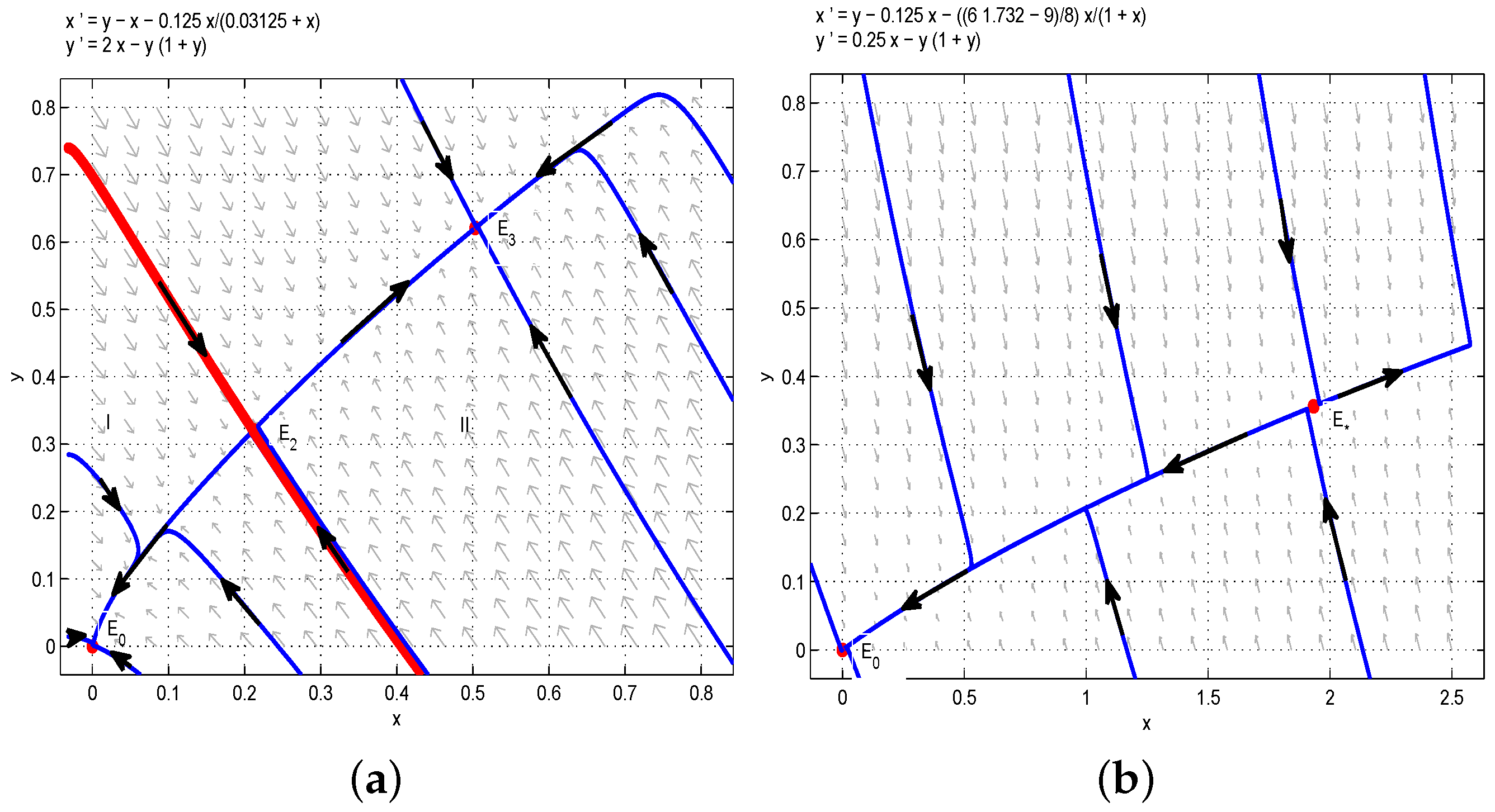
Through the above analysis and Figure 1, one could obtain that if , i.e., , the boundary equilibrium of Model (6) is unstable, and there are multiple stable states in the first quadrant. More precisely, if the birth rate of the juvenile species is much greater than the threshold , then two species can always coexist stably. In order to verify the above results, we take , then we have , and are stable nodes, and and are saddles. According to Figure 1a, the red line divides the first quadrant into two parts, denoted as I (left one) and II (right one). If the initial conditions lie in Region I, then all solutions tend to , which is a stable manifold, and both and are unstable manifolds. From the biological point of view, the juvenile and adult species will coexist if the initial conditions lie in Region I. Similarly, the juvenile and adult species will also coexist if the initial conditions lie in Region II. This is the first case of bistability phenomena, as shown in Figure 1a. If we take , , , then we have . Obviously, the model has two positive equilibria and (or ) and one unstable boundary equilibrium . Therefore, the model has two positive steady states, as shown in Figure 1b. Moreover, if we let , ,, then one could get , and the model has a positive equilibrium and an unstable boundary equilibrium , so the model has a positive steady state, as shown in Figure 1c.
This completes the proof. □
(II) The case :
Theorem 3.
If , Model (6) has no more than two internal equilibria. Furthermore,
Proof.
From Equations (9) and (17) and the property of the derivative of , one could easily get , , and , so is a saddle, is a stable node, and is a degenerate equilibrium, in which is a saddle node; the proof of the above conclusion is similar to Theorem 2, so here, we omit it.
Based on the above analysis and Figure 2, one could obtain that the model has a positive steady state. Two species will coexist permanently with some initial conditions, and under some initial conditions, two species will be extinct. In order to verify the above results, we choose , , , then we can obtain , and are stable nodes, and is a saddle. According to Figure 2a, the red line divides the first quadrant into two parts, denoted as I (left one) and II (right one). If the initial conditions lie in Region I, then all solutions tend to , which is a stable manifold, and is an unstable manifold. From the biological point of view, the juvenile and adult species will be driven to extinction if the initial conditions lie in Region I. However, if the initial conditions lie in Region II, then all solutions tend to , which is a stable manifold, and is an unstable manifold. From the biological point of view, the juvenile and adult species will coexist if the initial conditions lie in Region II. This is the second case of bistability phenomena, as shown in Figure 2a. In addition, when we take , then . It is easy to get that the model has a positive equilibrium , and the model has a positive steady state, as shown in Figure 2b.
This completes the proof. □
3. Global Stability of Equilibria
Theorem 4.
When holds, is globally asymptotically stable.
Proof.
By constructing a suitable Lyapunov function to prove Theorem 4, let:
It is obvious that the function is zero at , and V is positive if . We have:
Since , we have and if and only if . Then, satisfies Lyapunov’s asymptotic stability theorem, and we have that is globally asymptotically stable (see Figure 3).
This completes the proof of Theorem 4. □
Theorem 5.
When and hold, is globally asymptotically stable.
Proof.
To prove Theorem 5, taking the Dulac function , we have:
where:
By the Bendixson–Dulac discriminant, one could show that the model (6) has no limit cycle when , . On the other hand, When , is the unique boundary equilibrium of the model (6) and is a saddle. Therefore, according to the Poincaré–Bendixson theorem, is globally asymptotically stable (see Figure 4).
The proof of Theorem 5 is finished. □
4. Numerical Simulations
Example 1.
Consider the following single species stage structure model with Michaelis–Menten-type juvenile population harvesting:
here, we choose .
- (1)
- Let ; we have and , i.e., , then is globally asymptotically stable (see Figure 3). More precisely, when the birth rate of the juvenile species is much less than the threshold , both species will be driven to extinction.
- (2)
- Let ; by simple computation, we have and , i.e., , then is globally asymptotically stable (see Figure 4). That is to say, when when the birth rate of the juvenile species is much less than the threshold and if b satisfies , both species will coexist.
- (3)
- Let , and take , respectively, and . We have and , then both species will be driven to extinction. The influence of Michaelis–Menten-type harvesting on the model is shown in Figure 5. It shows that with b increasing, species will become extinct in a much shorter time; in other words, increasing the harvest area will accelerate the extinction of species.
- (4)
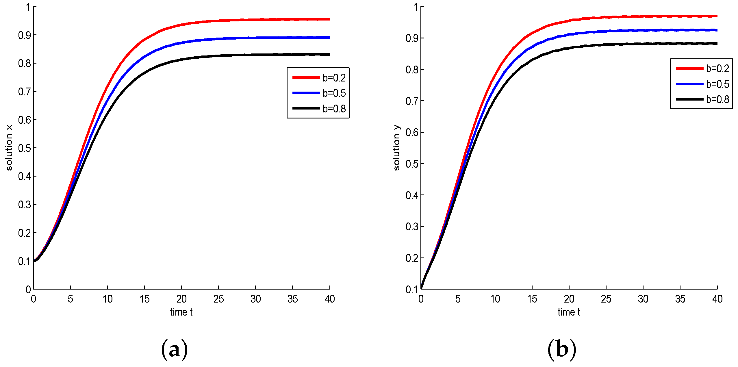
- Let , and take , respectively, and . We have and , then the model has a global asymptotically stable positive equilibrium . The influence of Michaelis–Menten-type harvesting on the model is shown in Figure 6. It shows that with b increasing, the density of species decreases; in other words, increasing the harvest area will reduce the species density.
5. Conclusions
A single species stage structure model with Michaelis–Menten-type juvenile population harvesting is discussed. The properties of the possible equilibria of the model are studied. Our results indicate that the Michaelis–Menten-type harvesting is more sensitive to the impact of model dynamics. It can not only reflect the harvesting process more realistically, but also make the dynamic behaviors of the model more complex than the linear harvesting in [15].
According to the analysis, we can get, compared with [33], that the model exhibits rich dynamic behaviors, and there are many kinds of positive steady states. The first type of bistability phenomenon shows that if , then the model is persistent when the initial value lies in the first quadrant. From the biological point of view, juvenile and adult species can coexist steadily. The second type of bistability phenomenon indicates that both species will coexist with some conditions, and under some conditions, both species will be extinct. Moreover, if i.e., , the boundary equilibrium is globally asymptotically stable; in other words, when the birth rate of the juvenile population is low enough, and the species will be driven to extinction. At the same time, our research also shows that increasing the harvest area will accelerate the rate of species extinction. In addition, if and , the system has a unique globally asymptotically stable internal equilibrium . That is to say, when the parameters meet certain conditions, harvesting does not affect the persistence of the model. However, increasing the harvest area will reduce the density of species. Our research is of great significance for decision makers in resource management of fisheries, forestry, and wildlife management. In other words, making a reasonable harvesting plan can not only ensure the maximization of economic benefits, but also maintain the sustainable development of resources.
Author Contributions
Writing—original draft, X.Y.; Writing—review & editing, Z.Z. and F.C. All authors equally contributed to this manuscript and approved of the final version. All authors read and agreed to the published version of the manuscript.
Funding
This work is supported by the Natural Science Foundation of Fujian Province (2019J01785).
Acknowledgments
The authors would like to thank the reviewers for their helpful comments and suggestions.
Conflicts of Interest
The authors declare no conflict of interest.
References
- Li, Z.; Han, M.; Chen, F. Global stability of stage-structured predator-prey model with modified Leslie-Gower and Holling-type II schemes. Int. J. Biomath. 2012, 6, 1250057. [Google Scholar] [CrossRef]
- Li, Z.; Han, M.; Chen, F. Global stability of a predator-prey system with stage structure and mutual interference. Discret. Contin. Dyn. Syst. B 2014, 19, 173–187. [Google Scholar] [CrossRef]
- Xiao, Z.; Li, Z.; Zhu, Z.; Chen, F. Hopf bifurcation and stability in a Beddington-DeAngelis predator-prey model with stage structure for predator and time delay incorporating prey refuge. Open Math. 2019, 17, 141–159. [Google Scholar] [CrossRef]
- Ma, Z.H.; Li, Z.Z.; Wang, S.F.; Li, T.; Zhang, F.P. Permanence of a predator-prey system with stage structure and time delay. Appl. Math. Comput. 2008, 201, 65–71. [Google Scholar] [CrossRef]
- Lei, C.Q. Dynamic behaviors of a stage-structured commensalism system. Adv. Differ. Equ. 2018, 2018, 301. [Google Scholar] [CrossRef] [Green Version]
- Zhang, F.; Chen, Y.; Li, J. Dynamical analysis of a stage-structured predator prey model with cannibalism. Math. Biosci. 2019, 307, 33–41. [Google Scholar] [CrossRef]
- Chen, F.; Xie, X.; Li, Z. Partial survival and extinction of a delayed predator-prey model with stage structure. Appl. Math. Comput. 2012, 219, 4157–4162. [Google Scholar] [CrossRef]
- Chen, F.; Chen, W.; Wu, Y.; Ma, Z. Permanece of a stage-structured predator-prey system. Appl. Math. Comput. 2013, 219, 8856–8862. [Google Scholar]
- Chen, F.; Wang, H.; Lin, Y.; Chen, W. Global stability of a stage-structured predator-prey system. Appl. Math. Comput. 2013, 223, 45–53. [Google Scholar] [CrossRef]
- Yue, Q. Permanence of a delayed biological system with stage structure and density dependent juvenile birth rate. Eng. Lett. 2019, 27, 1–5. [Google Scholar]
- Pu, L.; Miao, Z.; Han, R. Global stability of a stage-structured predator-prey model. Commun. Math. Biol. Neurosci. 2015, 2015, 5. [Google Scholar]
- Lin, Y.; Xie, X.; Chen, F.; Li, T. Convergences of a stage-structured predator-prey model with modified Leslie-Gower and Holling-type II schemes. Adv. Differ. Equ. 2016, 2016, 181. [Google Scholar] [CrossRef] [Green Version]
- Xue, Y.L.; Pu, L.Q.; Yang, L.Y. Global stability of a predator-prey system with stage structure of distributed-delay type. Commun. Math. Biol. Neurosci. 2015, 2015, 12. [Google Scholar]
- Ji, L.L.; Wu, C.Q. Qualitative analysis of a predator-prey model with constant-rate prey harvesting incorporating a constant prey refuge. Nonlinear Anal. Real World Appl. 2010, 11, 2285–2295. [Google Scholar] [CrossRef]
- Xiao, A.; Lei, C.Q. Dynamic behaviors of a non-selective harvesting single species stage structure system incorporating partial closure for the populations. Adv. Differ. Equ. 2018, 2018, 245. [Google Scholar] [CrossRef]
- Chen, B.G. Dynamic behaviors of a nonselective harvesting Lotka-Volterra amensalism model incorporating partial closure for the populations. Adv. Differ. Equ. 2018, 2018, 111. [Google Scholar] [CrossRef] [Green Version]
- Lei, C.Q. Dynamic behaviors of a nonselective harvesting May cooperative system incorporating partial closure for the populations. Commun. Math. Biol. Neurosci. 2018, 2018, 12. [Google Scholar]
- Chen, F.D.; Wu, H.L.; Xie, X.D. Global attractivity of a discrete cooperative system incorporating harvesting. Adv. Differ. Equ. 2016, 2016, 268. [Google Scholar] [CrossRef] [Green Version]
- Zhang, N.; Chen, F.; Su, Q.; Wu, T. Dynamic behaviors of a harvesting Leslie-Gower predator-prey model. Discret. Dyn. Nat. Soc. 2011, 2011, 473949. [Google Scholar] [CrossRef] [Green Version]
- Lin, Q.F. Dynamic behaviors of a commensal symbiosis model with nonmonotonic functional response and nonselective harvesting in a partial closure. Commun. Math. Biol. Neurosci. 2018, 2018, 4. [Google Scholar]
- Su, Q.Q.; Chen, F.D. The influence of partial closure for the populations to a nonselective harvesting Lotka-Volterra discrete amensalism model. Adv. Differ. Equ. 2019, 2019, 281. [Google Scholar] [CrossRef]
- Xie, X.; Chen, F.; Xue, Y. Note on the stability property of a cooperative system incorporating harvesting. Discret. Dyn. Nat. Soc. 2014, 2014, 327823. [Google Scholar] [CrossRef]
- Huang, X.; Chen, F.; Xie, X.; Zhao, L. Extinction of a two species competitive stage-structured system with the effect of toxic substance and harvesting. Open Math. 2019, 17, 856–873. [Google Scholar] [CrossRef]
- Liu, Y.; Xie, X.D.; Lin, Q.F. Permanence, partial survival, extinction, and global attractivity of a nonautonomous harvesting Lotka-Volterra commensalism model incorporating partial closure for the populations. Adv. Differ. Equ. 2018, 2018, 211. [Google Scholar] [CrossRef] [Green Version]
- Chen, B.G. The influence of commensalism on a Lotka-Volterra commensal symbiosis model with Michaelis–Menten-type harvesting. Adv. Differ. Equ. 2019, 2019, 43. [Google Scholar] [CrossRef] [Green Version]
- Kong, L.; Zhu, C.R. Bogdanov-Takens bifurcations of codimensions 2 and 3 in a Leslie Gower predator-prey model with Michaelis–Menten-type prey harvesing. Math. Methods Appl. Sci. 2017, 40, 6715–6731. [Google Scholar] [CrossRef]
- Yu, X.Q.; Chen, F.D.; Lai, L.Y. Dynamic behaviors of May type cooperative system with Michaelis–Menten-type harvesting. Ann. Appl. Math. 2019, 4, 3. [Google Scholar]
- Yu, L.; Guan, X.; Xie, X.; Lin, Q. On the existence and stability of positive periodic solution of a nonautonomous commensal symbiosis model with Michaelis–Menten-type harvesting. Commun. Math. Biol. Neurosci. 2019, 2019, 2. [Google Scholar]
- Liu, Y.; Zhao, L.; Huang, X.Y.; Deng, H. Stability and bifurcation analysis of two species amensalism model with Michaelis–Menten-type harvesting and a cover for the first species. Adv. Differ. Equ. 2018, 2018, 295. [Google Scholar] [CrossRef]
- Hu, D.P.; Cao, H.J. Stability and bifurcation analysis in a predator-prey system with Michaelis–Menten-type predator harvesting. Nonlinear Anal. Real World Appl. 2017, 33, 58–82. [Google Scholar] [CrossRef]
- Lin, Q.; Xie, X.; Chen, F.; Lin, Q. Dynamical analysis of a logistic model with impulsive Holling type-II harvesting. Adv. Differ. Equ. 2018, 2018, 112. [Google Scholar] [CrossRef]
- Xue, Y.L.; Xie, X.D.; Lin, Q.F. Almost periodic solutions of a commensalism system with Michaelis–Menten-type harvesting on time scales. Open Math. 2019, 17, 1503–1514. [Google Scholar] [CrossRef]
- Yu, X.Q.; Zhu, Z.L.; Lai, L.Y.; Chen, F. Stability and bifurcation analysis in a single-species stage structure system with Michaelis–Menten-type harvesting. Adv. Differ. Equ. 2020, 2020, 238. [Google Scholar] [CrossRef]
- May, R.M.; Beddington, J.R.; Clark, C.W.; Holt, S.J.; Laws, R.M. Management of multispecies fisheries. Science 1979, 205, 267–277. [Google Scholar] [CrossRef]
- Clark, C.; Mangel, M. Of schooling and the purse seine tuna fisheries. Fish. Bull. 1979, 77, 317–337. [Google Scholar]
- Zhang, Z.F.; Ding, T.R.; Huang, W.Z.; Dong, Z.X. Qualitative Theory of Differential Equation; Science Press: Beijing, China, 1992. [Google Scholar]
- Xiang, C.; Huang, J.; Ruan, S.; Xiao, D. Bifurcation analysis in a host-generalist parasitoid model with Holling II functional response. J. Differ. Equ. 2020, 268, 4618–4662. [Google Scholar] [CrossRef]
Figure 1.
(a) . The coexistence of three internal equilibria and one boundary equilibrium when : two stable nodes and and two saddles and . (b) . Two internal equilibria when : a stable node and a saddle node . (c) . is the only internal equilibrium, and it is the saddle node.
Figure 1.
(a) . The coexistence of three internal equilibria and one boundary equilibrium when : two stable nodes and and two saddles and . (b) . Two internal equilibria when : a stable node and a saddle node . (c) . is the only internal equilibrium, and it is the saddle node.
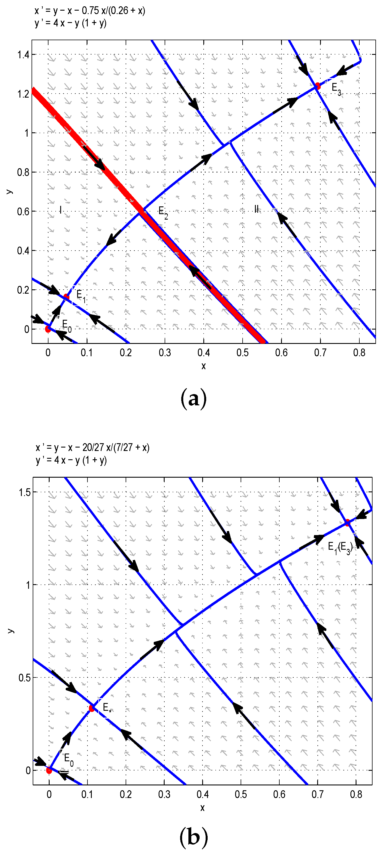
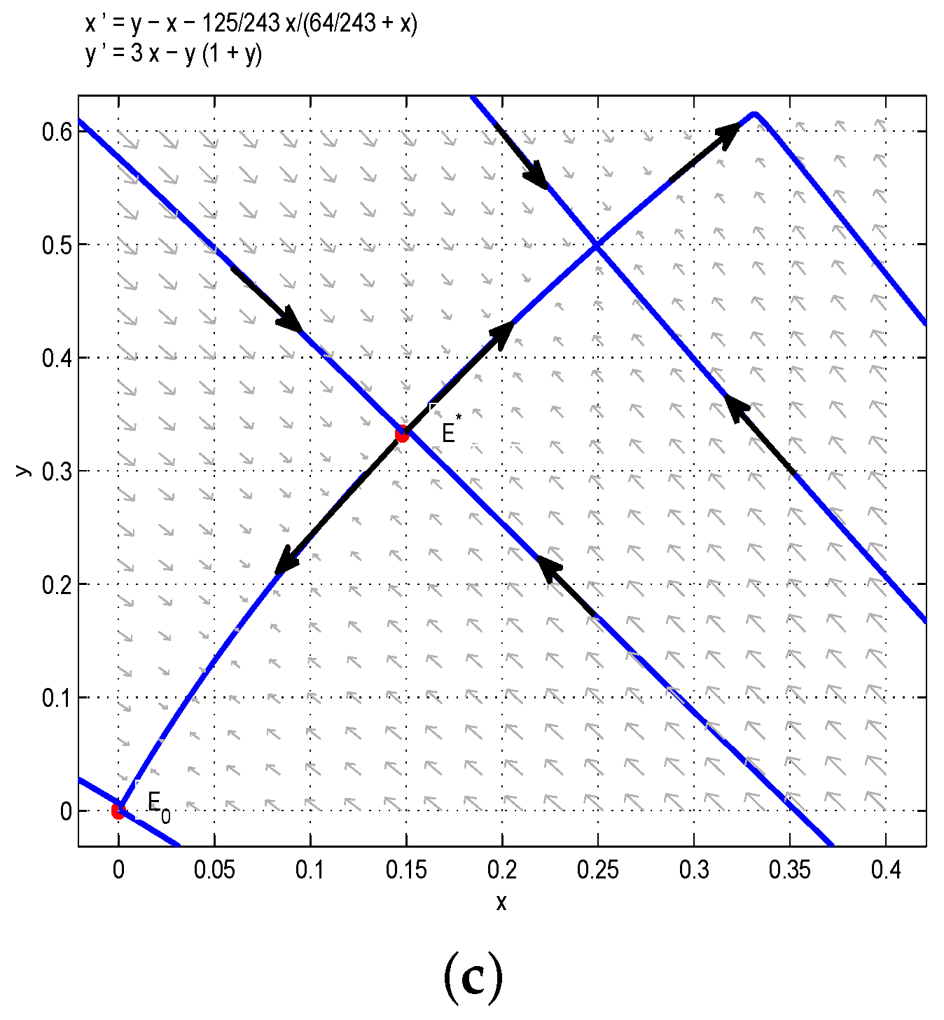
Figure 2.
(a) . Two coexisting internal equilibria and one boundary equilibrium when : two stable nodes and and a saddle . (b) . is the only internal equilibrium, and it is the saddle node.
Figure 2.
(a) . Two coexisting internal equilibria and one boundary equilibrium when : two stable nodes and and a saddle . (b) . is the only internal equilibrium, and it is the saddle node.

Figure 3.
System (6) has no internal equilibria, and a unique boundary equilibrium is globally asymptotically stable.
Figure 3.
System (6) has no internal equilibria, and a unique boundary equilibrium is globally asymptotically stable.
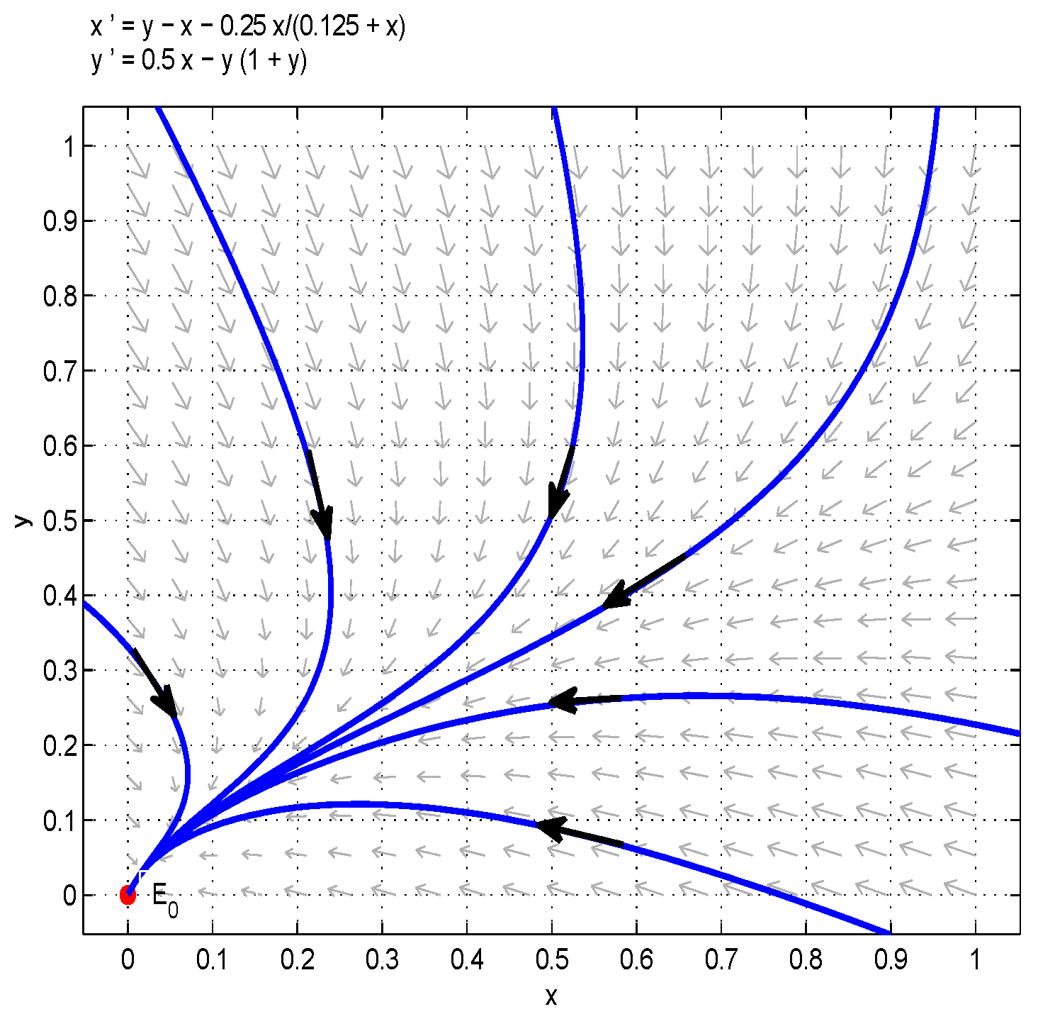
Figure 4.
A unique internal equilibrium is globally asymptotically stable when and .

Figure 5.
Take , respectively, and . In this case, is a stable node. (a) Juvenile species. Numerical simulation of juvenile species x of Model (22). (b) Adult species. Numerical simulation of adult species y of Model (22).
Figure 5.
Take , respectively, and . In this case, is a stable node. (a) Juvenile species. Numerical simulation of juvenile species x of Model (22). (b) Adult species. Numerical simulation of adult species y of Model (22).
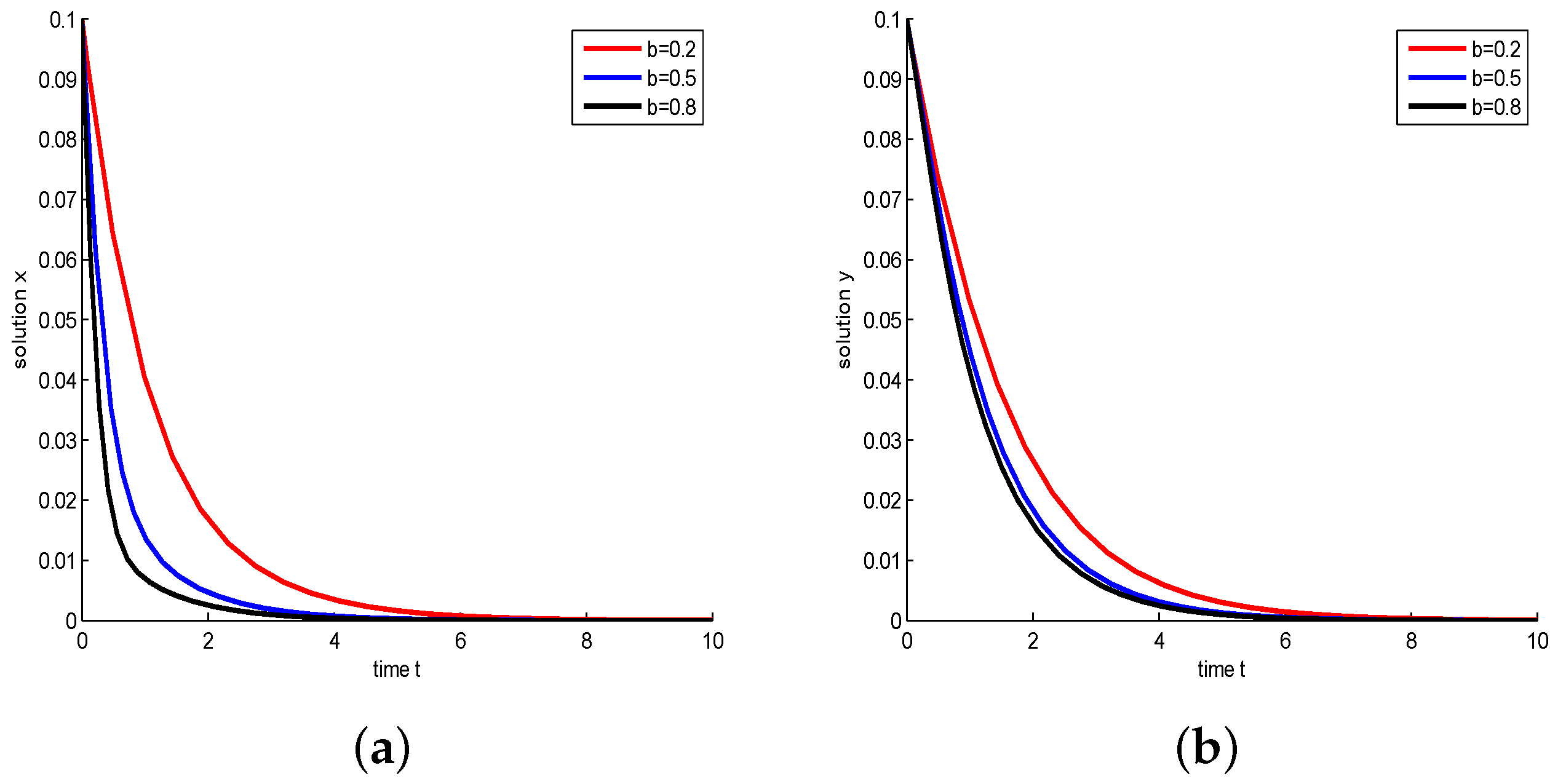
Figure 6.
Take , respectively, and . In this case, is a stable node. (a) Juvenile species. Numerical simulation of juvenile species x of Model (22). (b) Adult species. Numerical simulation of adult species y of Model (22).
Figure 6.
Take , respectively, and . In this case, is a stable node. (a) Juvenile species. Numerical simulation of juvenile species x of Model (22). (b) Adult species. Numerical simulation of adult species y of Model (22).

© 2020 by the authors. Licensee MDPI, Basel, Switzerland. This article is an open access article distributed under the terms and conditions of the Creative Commons Attribution (CC BY) license (http://creativecommons.org/licenses/by/4.0/).
Share and Cite
MDPI and ACS Style
Yu, X.; Zhu, Z.; Chen, F. Dynamic Behaviors of a Single Species Stage Structure Model with Michaelis–Menten-TypeJuvenile Population Harvesting. Mathematics 2020, 8, 1281. https://doi.org/10.3390/math8081281
AMA Style
Yu X, Zhu Z, Chen F. Dynamic Behaviors of a Single Species Stage Structure Model with Michaelis–Menten-TypeJuvenile Population Harvesting. Mathematics. 2020; 8(8):1281. https://doi.org/10.3390/math8081281
Chicago/Turabian StyleYu, Xiangqin, Zhenliang Zhu, and Fengde Chen. 2020. "Dynamic Behaviors of a Single Species Stage Structure Model with Michaelis–Menten-TypeJuvenile Population Harvesting" Mathematics 8, no. 8: 1281. https://doi.org/10.3390/math8081281
Note that from the first issue of 2016, this journal uses article numbers instead of page numbers. See further details here.