1. Introduction
The maximum weighted independent set (MWIS) problem is posed in a graph in which vertices have nonnegative weights. In its conventional variant, the problem consists of finding a subset of graph vertices that are not adjacent to each other and in which the sum of weights is as large as possible. There are many practical applications of such task, e.g., in resource allocation or in scheduling.
Although the conventional MWIS problem is NP-hard in general [
1], it still can be solved in polynomial time on some special classes of graphs, such as trees or interval graphs or apple-free graphs. Indeed, the paper [
2] specifies an algorithm for trees with linear complexity in terms of number of vertices. Next, in Reference [
3,
4,
5,
6,
7] we can find polynomial-time algorithms for interval or apple-free graphs.
In addition to the conventional variant, several robust variants of the MWIS problem can also be studied, where graph structure is fixed but vertex weights are uncertain. Since the conventional MWIS problem is NP-hard in general, it is clear that all its robust variants must also be NP-hard in general. But, as already noted, the conventional MWIS problem on some special classes of graphs can be solved in polynomial time. This gives rise to a hope that robust variants of the same problem on the same classes can also be solved more efficiently than in the general case.
To see if such hope is justified, it is necessary to analyze computational complexity of robust MWIS problem variants on particular types of graphs. Such analysis has already been done in Reference [
8,
9] for interval graphs—it turned out that almost all robust MWIS variants on interval graphs are NP-hard. To the best of our knowledge, there are no similar works in the literature dealing with trees or apple-free graphs.
In this paper, we are concerned with solving robust variants of the MWIS problem on trees. So, we are dealing simultaneously with robust optimization and with one of the special classes of graphs that are regarded as interesting from the computational point of view. Our goal is to study computational complexity of the considered robust variants on trees and also to design efficient algorithms for their solution.
In the paper, we will first explore relationships between trees and interval graphs. More precisely, we will demonstrate that none of those two classes of graphs is a subset of the other. This is important because it means that the available complexity results from Reference [
8,
9] regarding interval graphs cannot be applied to trees. Thus, a separate study of complexity is needed. In the second part of the paper, we will present our original complexity analysis dealing with robust MWIS problem variants on trees. Our results are analogous to those for interval graphs from Reference [
8,
9]. Consequently, they show that the considered problem variants on trees are again NP-hard. Thus again, we cannot expect exact polynomial-time solutions. In the last part of the paper, we will therefore concentrate on a custom-designed
heuristic, which solves robust MWIS problem variants on trees much faster than algorithms designed for general graphs.
It is well known that, for many combinatorial optimization problems, the simple structure of trees can assure algorithmic advantages for solving them efficiently [
1]. However, according to the results from this paper, this is not the case for the investigated robust problem variants. In this aspect, our problem variants are similar to some other hard problems posed on trees, such as the generalized minimum spanning tree problem [
10].
Apart from this introduction, the rest of the paper is organized as follows.
Section 2 lists precise definitions of the above used concepts, and establishes the difference between interval graphs and trees.
Section 3 contains our complexity results.
Section 4 describes our heuristic.
Section 5 reports on experimental evaluation of the algorithm. The final
Section 6 gives conclusions.
2. Definitions and Preliminaries
As already announced, in this paper we study the maximum weighted independent set problem. Its conventional variant is very well known and treated in many textbooks, e.g., Reference [
11,
12]. We give here some basic definitions for convenience.
Let be an undirected graph, where V is the set of vertices, and E the set of edges. An independent set of G is a subset X of V such that no two vertices in X are adjacent (connected by an edge from E).
Let be an undirected graph where its vertices have weights. Suppose that all weights are nonnegative integers. A maximum weighted independent set of G is an independent set of G in which the sum of vertex weights is as large as possible.
The problem of finding a maximum weighted independent set in a given weighted graph is called the (conventional) maximum weighted independent set problem (the MWIS problem).
Let us now say a few words about
robust optimization [
13,
14,
15,
16,
17]. It is a state-of-the-art paradigm for dealing with
uncertainty in problem parameters (e.g., vertex weights in our case). Such uncertainty occurs frequently in real-world applications where parameter values may depend on unpredictable future circumstances or perhaps cannot be measured accurately. In this paper, we adopt a particular approach to robust optimization, which has been described, e.g., in Reference [
13,
17].
In accordance with the adopted approach to robustness, uncertain values are expressed through a finite collection of scenarios, which can be listed explicitly or described implicitly through some kind of uncertainty set (e.g., a Cartesian product of integer intervals). Only the solutions that are feasible for all scenarios are taken into account. The “behavior” of any solution under any scenario is measured in some way. As the “robustly optimal” solution, the one is chosen in which overall behavior, measured over all scenarios, is the best possible.
Depending on the chosen behavior measure, the above procedure can lead to the application of different
criteria of robustness. There are three popular criteria, and according to Reference [
17], they are called absolute robustness, robust deviation, and relative robust deviation. In some other literature, e.g., Reference [
13], the same criteria are referred to as max-min (min-max), min-max-regret, and relative min-max regret, respectively. Here are the definitions.
An absolute robust solution is the one in which the worst (conventional) objective-function value, measured over all scenarios, is the best among all feasible solutions.
A robust deviation solution is the one in which the maximum deviation from the conventional optimum, measured over all scenarios, is the smallest among all feasible solutions.
A relative robust deviation solution is the one in which the maximum relative deviation from the conventional optimum, measured over all scenarios, is the smallest among all feasible solutions.
Each of the three robustness criteria shown above can further on be extended by using the corresponding ordered-weighted-averaging aggregation (OWA) criterion. The idea is that the assessment of a given solution should not be based only on the worst measured value of objective function or deviation. Instead, a convex combination of several “bad” values should be taken into account. As an OWA solution, the one is chosen in which convex combination is the best. More information about OWA criteria can be found in Reference [
16].
In this paper, we apply our adopted robustness approach to the MWIS problem. Thereby, the graph structure is assumed to be stable, only vertex weights are considered as uncertain. Consequently, each scenario is simply an n-tuple of nonnegative integers, where n is the number of vertices in the graph. In any scenario, the first integer defines the weight of the first vertex, the second integer is the weight of the second vertex, etc. By applying the three previously mentioned robustness criteria, we obtain three different robust variants of the MWIS problem. The next paragraph gives precise definitions of those variants.
For a graph , let S be the collection of all scenarios for its vertex weights. Denote with the weight of an independent set (i.e., the sum of weights of its vertices) under scenario . Let be the maximum weight of an independent set under scenario s. Assume that is (this is, in fact, always true except for trivial problem instances). Then:
An absolute robust solution for the MWIS problem is an independent set that maximizes the function over the whole collection of possible independent sets X.
A robust deviation solution for the MWIS problem is an independent set that minimizes the function over the whole collection of possible independent sets X.
A relative robust deviation solution for the MWIS problem is an independent set that minimizes the function over the whole collection of possible independent sets X.
In the remaining part of this section, we define precisely two previously mentioned special classes of graphs. Indeed, here are the definitions.
An undirected graph G is a tree if it is connected and acyclic. Or, equivalently, an undirected graph G with n vertices is a tree if it is connected and its number of edges is .
A tree is usually organized in a hierarchy, so that one vertex is chosen to be the root, its neighbors become its children, remaining neighbors of children become children’s children, etc. Then, any vertex can have 0, 1 or more children. The root has no parent, and any other vertex has exactly one parent. Vertices with no children are called leaves.
Let , denote a closed interval, where and . An undirected graph with vertices is called interval graph for a finite family of intervals on the real line if there is a one-to-one correspondence between and V such that two intervals of have non-empty intersection if and only if their corresponding vertices in V are adjacent to each other.
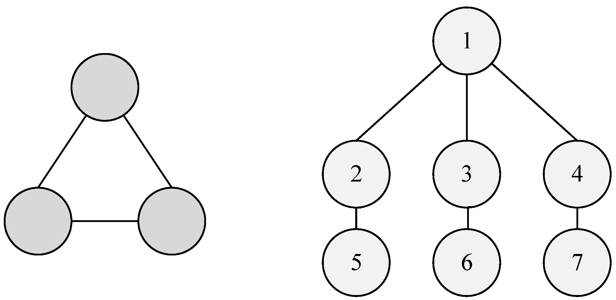
It is important to point out that none of the two considered classes of graphs is a subset of the other. This fact is demonstrated by
Figure 1, where we can see an interval graph that is not a tree and also a tree that is not an interval graph.
Let us explain
Figure 1 in more detail. The graph on the left is obviously not a tree because it has a cycle, but on the other hand, it is an interval graph since it corresponds, e.g., to a family
. The graph on the right is obviously a tree, but it is not an interval graph since there exists no corresponding family of intervals. Namely, any attempt to construct such a family leads to a contradiction. Indeed, let us try to construct such intervals. Denote with
the interval corresponding to vertex
i. Our attempt is illustrated by
Figure 2.
Consider first
,
, and
; since their vertices are not adjacent, they should be disjunct and placed on the real line in some sequence. Without any loss of generality, we can assume that
is on the left,
in the middle, and
on the right, as shown in the middle part of
Figure 2 (otherwise, we could renumber the vertices).
Next, consider
. Since vertex 1 is adjacent to vertices 2, 3, and 4,
should overlap with all three intervals
,
, and
. More precisely, the left endpoint of
cannot be larger than the right endpoint of
since, otherwise, the two intervals would not overlap. Similarly, the right endpoint of
cannot be smaller than the left endpoint of
. So, the situation looks as shown in the upper part of
Figure 2. Consequently,
must be a subset of
.
Finally, we consider
. Since vertices 3 and 6 are adjacent,
should overlap with
, as shown in the lower part of
Figure 2. But since
is a subset of
, it means that
must also overlap with
. This is a contradiction with the fact that vertices 1 and 6 are not adjacent.
3. Complexity Issues
A natural question one would like to answer is whether there exists an exact algorithm, similar to the one from Reference [
2], which would solve robust variants of the MWIS problem on trees in polynomial time. Unfortunately, the answer is in most cases negative due to the following theorems. They are proved by polynomial reduction of the standard
2-partition problem to our robust variants. We start with the definition of 2-partition:
Instance: a list of positive integers .
Question: is there a subset of indices such that ?
It is well known [
1] that the 2-partition problem is NP-complete.
Theorem 1. Finding an absolute robust solution for the MWIS problem on trees is NP-hard, even with only two discrete scenarios.
Proof. Let us consider an instance of the 2-partition problem specified by positive integers
. Denote with
T the sum
. We construct the corresponding MWIS problem instance with two scenarios on the tree shown in
Figure 3. The first scenario is specified as follows:
The second scenario is specified as follows:
A nontrivial independent set (i.e., one that cannot be extended by adding more vertices) is formed so that exactly one (upper or lower) vertex is chosen in each vertical segment from
Figure 3. The root may or may not be chosen, but it is irrelevant since its weight is 0. Here follow some observations.
If the selected independent set contains many upper vertices, it will have a large weight under the first scenario but a small weight under the second scenario. Thus, its minimum weight over scenarios will be small, so that it will not be an absolute robust solution.
If the selected independent set contains many lower vertices, it will have a large weight under the second scenario but a small weight under the first scenario. Again, its minimum weight over scenarios will be small, so that it again will not produce an absolute robust solution.
An absolute robust solution (max-min) is achieved when the sum of weights of the chosen upper vertices is approximately equal to the sum of weights of the chosen lower vertices, since then the minimum over scenarios is as large as possible.
From the above observations, we can deduce the following. If the robust objective function value (max-min) happens to be exactly , then a 2-partition of exists. If it is , then a 2-partition does not exist.
It means that, by solving the robust MWIS problem instance, we obtain the solution of the 2-partition instance. □
Theorem 2. Finding a robust deviation solution for the MWIS problem on trees is NP-hard, even with only two discrete scenarios.
Proof. Let us consider an instance of the 2-partition problem specified by positive integers
. Denote again with
T the sum
. We construct the corresponding MWIS problem instance in the same way as in the proof of Theorem 1, i.e., the tree looks as shown in
Figure 3 and the two scenarios are the same. Nontrivial independent sets are also formed in the same way as before. Now, we can observe the following.
The optimal conventional solution under the first scenario is obtained by choosing the upper vertex within each vertical segment from
Figure 3. The weight of that solution is
T.
The optimal conventional solution under the second scenario is obtained by choosing the lower vertex within each vertical segment from
Figure 3, and its weight is again
T.
Let us consider any independent set
X. Let
I be the set of indices of vertical segments from
Figure 3 where
X has chosen the upper vertex. Then, the “regret” for
X under the first scenario is equal to
, and the regret for
X under the second scenario is
.
If X contains many upper vertices, it will have a small regret under the first scenario but a large regret under the second scenario, so that its maximal regret over both scenarios will be large.
If X contains many lower vertices, it will have a large regret under the first scenario and a small regret under the second scenario. Again, its maximal regret over both scenarios will be large.
A robust deviation solution (min-max regret) is achieved when is approximately equal to , since then the maximal regret over both scenarios is as small as possible and .
From the above observations, we can deduce the following. If the robust objective function value (min-max regret) happens to be exactly , then a 2-partition of exists. If it is , then a 2-partition does not exist.
Thus, by solving the constructed robust MWIS problem instance, we solve the given 2-partition instance. □
Theorem 3. Finding a relative robust deviation solution for the MWIS problem on trees is NP-hard, even with only two discrete scenarios.
Proof. It is almost the same as for Theorem 2. For a given 2-partition problem instance specified by positive integers , we construct again the same MWIS problem instance (the same tree and scenarios). Nontrivial independent sets are formed in the same way as before, and the optimal conventional solutions under particular scenarios are the same. T again stands for . But now we can observe the following.
From the above observations, we can deduce the following. If the robust objective function value (min-max relative regret) happens to be exactly , then a 2-partition of exists. If it is , then a 2-partition does not exist.
Thus, by solving the constructed robust MWIS problem instance, we solve the given 2-partition instance. □
With the above three theorems, we have proved that the absolute robust variant and the (relative) robust deviation variants of the MWIS problem on trees are NP-hard. Since the involved three robustness criteria are special cases of the corresponding OWA criteria, we immediately obtain the following consequence.
Corollary 1. For any of the three robustness criteria, finding the respective OWA solution for the MWIS problem on trees is NP-hard, even with only two discrete scenarios.
Next, we can combine the complexity results from this section with the equivalency results from Reference [
18]. In this way, we can immediately prove some assertions regarding robust variants of the so-called minimum-weight vertex cover problem (MWVC) problem on trees. As it is well known [
11], MWIS and MWVC problems are closely related, in fact equivalent, if their conventional variants are considered. However, as shown in Reference [
18], robust variants of the same problems are not always equivalent, so that one cannot be sure that MWVC variants should have the same complexity as their MWIS counterparts. Still, combination of Proposition 2 from Reference [
18] with our Theorem 1 brings the following consequence.
Corollary 2. Finding an absolute robust solution for the MWVC problem on trees is NP-hard, even with only two discrete scenarios.
The above corollary follows because the MWIS problem instance used in the proof of our Theorem 1 can (polynomially) be reduced to the corresponding MWVC problem instance. Such reduction is correct since the involved instances satisfy the restriction from Reference [
18] regarding scenarios. Similarly, Proposition 8 from Reference [
18] can be combined with our Theorem 2, thus giving an additional consequence.
Corollary 3. Finding a robust deviation solution for the MWVC problem on trees is NP-hard, even with only two discrete scenarios.
It is easy to see that an analogue claim regarding relative robust deviation solution of the MWVC problem on trees is also true. Such a claim can be proved directly by a similar (but slightly modified) construction, as in our Theorem 3.
So far, we have assumed that uncertainty in our robust MWIS problem variants is captured through discrete scenarios. Let us now say a few words about situations where uncertainty is expressed by intervals. More precisely, we now assume that the weight of a vertex can take any value from a given integer interval. Vertex weights are chosen independently from each other. Thus, the set of scenarios
S is implicitly given as the full Cartesian product of all intervals. Such scenario set can be combined with any of the three previously considered robustness criteria. In this way, robust variants of the MWIS problem are obtained, which are special cases of the previously considered variants, having rather large but regular sets of scenarios. Such special and regular variants deserve separate consideration since their complexity could be different (smaller) than in more general situations. Indeed, it is clear that combination of absolute robustness with interval uncertainty on trees gives a variant of the MWIS problem that can be solved in polynomial time—this fact is a consequence of Proposition 4 from Reference [
18] or Proposition 7.4 from Reference [
9]. More precisely, the sought robust solution coincides with the conventional solution according to the so-called minimum scenario (where each vertex has the smallest weight from its interval).
4. Algorithms
At the beginning of this section, we will first briefly describe the exact algorithm for solving the conventional MWIS problem on trees from Reference [
2]. Namely, the construction from Reference [
2] will serve as an inspiration for our own algorithm described in the second part of the section.
As previously mentioned, the algorithm from Reference [
2] has a linear complexity. In more detail, the algorithm visits each vertex
in a given tree just once, and it constructs two corresponding independent sets:
An independent set for the subtree rooted at that has the greatest weight and that contains . Such set will be called the inclusive independent set.
An independent set for the subtree rooted at that has the greatest weight, and that does not contain . Such set will be called the exclusive independent set.
In its i-th step, the algorithm constructs the above described two independent sets for vertex by using the previously constructed independent sets for children of . The construction is done in the following way.
The inclusive independent set for is obtained as the union of exclusive independent sets for children of , plus itself.
The exclusive independent set for is obtained as a union of either inclusive or exclusive independent sets for children of . For each child, the one with greater weight is chosen.
As its final solution for the whole tree, the algorithm chooses the better among the two independent sets obtained for the root. Comparison is again done according to weights. It is easy to prove that the described algorithm is correct, i.e., it really constructs a solution that must be optimal in the conventional sense.
In the remaining part of this section, we propose a new heuristic for solving robust MWIS problem variants on trees. It will be called population algorithm. Similarly as the exact algorithm from the first part of the section, it takes into account the special structure of the involved graph (i.e., a tree). Again, it visits vertices of a tree and constructs independent sets for the corresponding subtrees. However, unlike the previous algorithm, it does not produce only one exclusive or inclusive set per vertex but collections of such sets.
More precisely, for a given tree, the population algorithm visits each vertex of that tree exactly once and constructs two corresponding collections of independent sets.
A collection of independent sets for the subtree rooted at that are considered “good” according to the chosen robustness criterion. Thereby, each of those independent sets contains . Such collection is called the inclusive population.
A collection of independent sets for the subtree rooted at that are considered “good” according to the chosen robustness criterion. Thereby, none of those independent sets contains . Such collection is called the exclusive population.
In its i-th step, the algorithm constructs the above described two populations for vertex by using previously constructed populations for children of . The construction is done in the following way.
A member of the inclusive population for is assembled as a union, where for each child of one member of its exclusive population is added. Vertex is also put into the union. The selection of particular members from children populations is done randomly but not with equal probability. Independent sets that are better according to the used robustness criterion have more chance to be chosen. In more detail, all independent sets are represented by sub-segments in which the lengths correspond to the respective objective-function values. Next, a uniformly distributed random number is generated in which the range covers the whole segment. The random number will more likely fall into a sub-segment with greater length.
A member of the exclusive population for is created as a union, where for each child of one member of its inclusive or exclusive population is added. Again, independent sets from children’s populations are chosen randomly, but those sets that are better according to the used robustness criterion are more likely to be selected. Random choice is implemented in the same way as for the members of inclusive population.
Note that the above described construction does not ensure uniqueness of solutions in the inclusive or exclusive population. Indeed, some population members could appear more than once if they are more fit. Comparing a newly created member with a list of already existing members would be an expensive operation. Hence, allowing to have copies of some solutions both requires less computing time and gives advantage to better solutions, i.e., it does not force filling a population with different solutions when they are bad just for the sake of the uniqueness.
As its final solution for the whole tree, our population algorithm selects the best independent set found within both populations that have been constructed for the root. The comparison of sets is again done according to the involved robustness criterion.
The described algorithm is called population algorithm since it creates populations of independent sets for each subtree of a tree. Its complexity is , where n is again the number of vertices in the tree.
For calculating the objective function in case of (relative) robust regret, we need optimal solutions for the corresponding conventional problems, i.e., we need optimal solution values for each scenario. Those values are obtained by using the exact algorithm from Reference [
2] described at the beginning of this section. Although each step of the algorithm finds a solution in a subtree, its value is evaluated as it was a solution for the whole tree. In more detail, for each scenario the regret of some solution in a subtree is calculated as difference between the global optimal value for that scenario and the solution value. Similarly, relative regret is calculated as difference between the global optimal value and the solution value divided by the global optimal value. There are two reasons why we prefer global rather than local optima:
It requires less memory. Moreover, it would be almost impossible to store simultaneously optimal solutions for all subtrees in case of a large tree.
Our aim is to find the global robustly optimal solution, hence comparing “partial” solutions to global conventional solutions would hopefully lead more directly to the desired goal.
In order to assure good performance of the described algorithm, it is very important to choose the right size for populations. If populations are too small, there will be not enough diversity of solutions to be carried from one level of the tree to the next level. On the other hand, if populations are too big, the algorithm will spend too much memory and time.
For vertices at lower levels of a tree, such as leaves, it does not make sense to have large populations. Indeed, the exclusive population for a leaf can contain only the empty set, and the inclusive population can have just one set containing only that leaf. In our current implementation of the algorithm, the population size first grows with each level until it reaches 12, then it is fixed until the end of computation. More precisely, the exclusive population for a vertex will have the size equal to the sum of sizes of exclusive populations for children of . When such size exceeds 12, it is reduced to 12. The same rule also applies for inclusive populations.
Next, in order to assure an even better accuracy, our current implementation of the algorithm forces two greedy choices of independent sets within any inclusive population. More precisely:
Similarly, two greedy choices are also done during the construction of an exclusive population. To summarize, in our present implementation, any population with size 12 must contain the described two “greedy” independent sets, and only the remaining 10 members are created by random choice.
Finally, let us note that our population algorithm is interesting because it combines characteristics of three different algorithm paradigms [
19,
20]:
- (1)
Dynamic programming. We calculate a table of partial solutions. We use results of previous calculations within subsequent calculations.
- (2)
Greedy approach. We implicitly assume that an independent set will be a “good” solution for the whole tree if it is assembled from parts that are “good” solutions for subtrees of that tree.
- (3)
Evolutionary computing. We use populations of solutions instead of single solutions. Our populations evolve during algorithm execution. Better solutions have more chance to survive and evolve.
Now follows a concrete example illustrating how our population algorithm works. Our example is large enough to be nontrivial but still small enough to be verifiable by hand. We consider the weighted tree with 14 vertices from
Figure 4. Each vertex is labeled with two weights that correspond to two scenarios. For the sake of simplicity, the population size is reduced to 5. Thereby, the first member of a population is a union of best members from the respective children’s populations, the second member is a union of average-best members from the respective children’s populations, and the remaining three members are created by random choice. We will use the absolute robustness criterion (max-min). One possible outcome of the algorithm is represented in
Table 1.
Let us now analyze
Table 1 in more detail. As stated before, the inclusive and exclusive population for a leaf are the sets consisting of that leaf and an empty set, respectively. It is also easy to create both populations for vertices 4 to 7. Namely, vertices 4 to 7 have only leaves for their children, which means that they have only one option how to construct a member of their inclusive population: they must put themselves into a single-element set. The tree from
Figure 4 is rather simple, but if we had a tree with branches of different lengths, we would obtain more versatile populations.
Although for vertices in higher levels, such as 0 and 2, we have more options for population members, some members are appearing more than once. It is because they are more fit for global solution and, again, because the tree from
Figure 4 is small. In a bigger tree, we would again have more versatile populations.
Let us explain in more detail how the inclusive and exclusive population are created for vertex 2. First, we create the inclusive population. The first member is a union of the best members from the exclusive populations of its children, plus vertex 2. For vertices 5 and 6, being children of vertex 2, the best members from their exclusive populations are and , respectively. Thus, the best member of the inclusive population of vertex 2 is . The second member is the average-best member. It is created similarly, but instead of taking the best members of its children, we take into consideration the average-best members of its children. Other three members are created randomly, as described on page 8 of this paper.
Now, we will explain how the exclusive population is created. The first member is a union, where for each child the best member of its inclusive or exclusive population is added. For vertex 5, we have an option to choose between or . Namely, the independent sets and are the best members of the inclusive and exclusive population belonging to vertex 5, respectively. The independent set is better (it has a greater value of the objective function); hence, we chose , rather than . Next, we make a similar choice for vertex 6. By combining both choices, we obtain that the best member of the exclusive population for vertex 2 equals . The second member is again the average-best member. It is created similarly as the average-best member for the inclusive population, but now we must take into consideration the average-best members of both the inclusive and exclusive population. The remaining three members are again created randomly, as described on page 8 of this paper.
The algorithm ends with choosing either the inclusive or exclusive member from the populations obtained for the root. Among all those sets, has the greatest robust (max-min) objective function value. In the considered case, the algorithm has found a solution which is truly optimal, i.e., the found solution coincides with the exact robust solution. This gives rise to a hope the algorithm will also perform reasonably well on bigger and more complex problem instances. The actual performance on larger instances will be measured experimentally in the next section.
5. Testing and Results
In this section, we will present the results of experimental evaluation of our population algorithm from
Section 4. It would be nice if we could test the algorithm on some well-known benchmark problem instances for robust variants of the MWIS problem. However, to the best of our knowledge, such benchmarks do not exist, specially not on trees. Therefore, we generated our own nine test groups, each comprising 30 problem instances. Those instances are based on random trees consisting of 30,000, 60,000, and 90,000 vertices. As we wanted to test different tree configurations, for each number of vertices, we produced 3 groups of trees. Thereby, vertices from the first, second, and third such group can have a maximum of 5, 10, and 15 children, respectively. In all nine test groups, each problem instance comprises 10 discrete scenarios for vertex weights. Thereby, each individual weight ranges between 1 and 1000. A full specification of all problem instances can be found in our repository at the address
http://hrzz-rodiopt.math.pmf.unizg.hr.
The population algorithm was implemented in the Java programming language [
21]. The program is available in the same repository as the problem instances. Among different state-of-the art programming languages, we chose Java since we wanted to take advantage of its garbage collector. Indeed, garbage collection is needed because our algorithm uses a lot of memory to store populations of independent sets. When the algorithm moves to a higher level of a tree, the memory used for the previous level must be deallocated; otherwise, we would run out of memory.
To measure performance of our population algorithm, we used the results obtained with the well known software package CPLEX [
22] for comparison. Note that the chosen problem instances are large enough to be nontrivial but still small enough to be solved exactly by CPLEX. Both our implemented algorithm and CPLEX were installed on the same computer with an Intel Core i5-6600K @ 3.50 GHz processor and 16 GB of RAM, running a 64-bit operating system.
Some robust variants of the MWIS problem (i.e., the deviation and the relative deviation variant) require solutions of the conventional MWIS problem instances that correspond to particular scenarios. Namely, such conventional solutions determine parameters within the corresponding robust objective functions. As explained in
Section 4, the needed conventional solutions can be calculated very quickly by using the exact polynomial-time algorithm from Reference [
2].
Since our population algorithm is a heuristic, the most important indicator of its performance is its accuracy. In our tests involving robust problem instances, we measured the accuracy by computing the relative errors of approximate solutions versus exact (truly optimal) solutions. More precisely, in each test, we computed relative difference between the robust objective-function value achieved with our approximate solution and the corresponding optimal robust objective-function value assessed by CPLEX.
In our tests, we solved each of the 30 problem instances from each of the nine test groups according to each of the three robustness criteria: absolute robustness and (relative) robust deviation. Since the population algorithm is nondeterministic, its repeated execution on the same input data usually does not produce the same solutions. Therefore, all computations with the population algorithm were repeated 10 times.
The results of our tests regarding accuracy are summarized in
Table 2,
Table 3 and
Table 4. Each table corresponds to one of the three robustness criteria. Any table is divided into two halves—they both contain average errors for nine different test groups, i.e., nine different combinations of the number of vertices versus the maximum number of children per vertex. The difference between the two parts within the same table is as follows. In the upper part, the errors obtained through 10 repeated executions of the same computational task were averaged. In the lower part, only the best (smallest) error obtained in 10 repeated executions was recorded. In both parts, the collected values (average or best errors) were further averaged over test groups.
Let us first analyze
Table 2, which refers to absolute robustness. We can see that, with that criterion, the algorithm performs very well. Indeed, average relative errors are less than 0.3%. We can observe that errors become lower when the number of vertices increases. It means that our algorithm is able to solve very large problem instances accurately. In addition, it is interesting to note that errors drop when the maximum number of children increases. More children means fewer levels in trees. Although errors are smaller for outspread trees, we pay for this with longer execution times, as it will be seen in
Table 5.
Next, we analyze the results from
Table 3 and
Table 4, corresponding to robust deviation and relative robust deviation, respectively. Both tables contain values that do not differ significantly; therefore, we analyze them together. We can see that the algorithm still works reasonably well since it produces errors between 4% and 8%. Moreover, errors again become lower when the number of vertices increases—this is similar to the case of absolute robustness. However, contrary to absolute robustness, errors now increase if the number of children becomes larger.
If we compare the best relative errors within
Table 2,
Table 3 and
Table 4 to the corresponding average relative errors within the same table, we see that there is no significant difference. Indeed, although the population algorithm is randomized, its solutions do not show much diversity. It seems that the algorithm is quite firmly guided by its greedy components. There is nothing similar to mutation which would bring more volatility.
The obtained results become even more attractive when we take execution time into account.
Table 5,
Table 6 and
Table 7 present the execution times for all three robustness criteria. Each table has two parts, which correspond to the population algorithm and CPLEX, respectively.
From
Table 5,
Table 6 and
Table 7, we can see that the population algorithm is considerably faster than CPLEX. The speedup is between 70 and 250 for absolute robustness, between 60 and 850 for robust deviation, and from 45 to 425 for relative robust deviation.
We can also notice that CPLEX needs more time for (relative) robust deviation than for absolute robustness. In addition, CPLEX spends much more time when the number of children is small. This is according to our expectations because, in such situations, exact branch-and-bound methods used by CPLEX become more demanding.
At the end of this section, let us mention that we have also tested our algorithm on trees with only a few hundreds of vertices. On such small trees, the algorithm often finds exact solutions, i.e., the same solutions as CPLEX. But then CPLEX is also extremely fast, so that in such cases, our heuristic does not show any advantage.


