Energetic-Property-Preserving Numerical Schemes for Coupled Natural Systems

Abstract

In this paper, we propose a method for deriving energetic-property-preserving numerical schemes for coupled systems of two given natural systems. We consider the case where the two systems are interconnected by the action–reaction law. Although the derived schemes are based on the discrete gradient method, in the case under consideration, the equation of motion is not of the usual form represented by using the skew-symmetric matrix. Hence, the energetic-property-preserving schemes cannot be obtained by straightforwardly using the discrete gradient method. We show numerical results for two coupled systems as examples; the first system is a combination of the wave equation and the elastic equation, and the second is of the mass–spring system and the elastic equation.

1. Introduction

Recently, against the background of complication of designing industrial products, the necessity of coupled simulation of plural phenomena according to different equations has increased. To carry out such simulations, first, it is necessary to construct and discretize appropriate mathematical models before numerical calculations. However, even if the equations for individual phenomena are known, naive combination of the equations easily results in violating important law of physics such as the energy-conservation law [1,2].

In this paper, we propose energetic-property-preserving numerical schemes for coupled models of two given natural systems. Popular models for coupled systems are the Port-Hamiltonian systems [3]. From the viewpoint of geometric mechanics, in this approach, the equations are described by using the Dirac structure, which is a geometric structure generalized from the symplectic structure and the Poisson structure [4]. This structure describes the energy transfer between the systems, thereby deriving the model equation in such a way that the energetic property of the coupled systems is preserved. It is also known that the resultant coupled system is also port-Hamiltonian and hence models for large coupled systems can be derived in a systematic way. In addition, the Lagrangian formalism of this approach is also reported [5,6,7].

Regarding numerical schemes for the port-Hamiltonian systems, energy-preserving and passivity-consistent numerical schemes were proposed by Celledoni and Høiseth [8]. Focusing on a discrete energy balance equation and the stability under interconnection, Celledoni and Høiseth proposed a definition of discrete port-Hamiltonian systems. Port-Hamiltonian systems are typically written as

$$\begin{array}{c}\hfill \frac{\mathrm{d}x}{\mathrm{d}t}=\left(B\right(x)-R(x\left)\right)\nabla H\left(x\right)+G\left(x\right)u,x\left(0\right)=x_0,y=G{\left(x\right)}^{\top }\nabla H\left(x\right),\end{array}$$

(1)

where $x\in {\mathbb{R}}^n$ is the state variables, $u\in {\mathbb{R}}^m$ is the input, and $y\in {\mathbb{R}}^m$ is the output. $B\left(x\right)$ is a skew-symmetric matrix, which is often corresponding to the Hamiltonian structure of the underlying systems. $G\left(x\right)$ is a $n\times m$ matrix. $H:{\mathbb{R}}^n\to \mathbb{R}$ is typically an energy function. $R\left(x\right)$ is a positive definite matrix, which is corresponding to the dissipation property of the system. For conservative systems, $R\left(x\right)=0$. In [8], two conservative systems, one of which is supposed to be given while the other is a controller to be designed, are assumed to be interconnected by

$$\begin{array}{cc}\hfill & \frac{\mathrm{d}x}{\mathrm{d}t}=B\left(x\right)\nabla H\left(x\right)+G\left(x\right)u,x\left(0\right)=x_0,y=G{\left(x\right)}^{\top }\nabla H\left(x\right),\hfill \\ \hfill & \frac{\mathrm{d}\tilde{x}}{\mathrm{d}t}=\tilde{B}\left(\tilde{x}\right)\nabla H\left(\tilde{x}\right)+\tilde{G}\left(\tilde{x}\right)\tilde{u},\tilde{x}\left(0\right)={\tilde{x}}_0,\tilde{y}=\tilde{G}{\left(\tilde{x}\right)}^{\top }\nabla \tilde{H}\left(\tilde{x}\right),\hfill \\ \hfill & u=\tilde{y},\tilde{u}=-y\hfill \end{array}$$

(2)

so that the total energy is preserved:

$$\begin{array}{c}\hfill \frac{\mathrm{d}}{\mathrm{d}t}(H+\tilde{H})=y^{\top }u+{\tilde{y}}^{\top }\tilde{u}=y^{\top }\tilde{y}-{\tilde{y}}^{\top }y=0.\end{array}$$

(3)

In fact, the above system is shown to be

$$\begin{array}{c}\hfill \frac{\mathrm{d}}{\mathrm{d}t}\left(\begin{array}{c}x\\ \tilde{x}\end{array}\right)=C(x,\tilde{x})\left(\begin{array}{c}{\nabla }_x(H+\tilde{H})\\ {\nabla }_{\tilde{x}}(H+\tilde{H})\end{array}\right)\end{array}$$

(4)

with a skew-symmetric matrix C. By using this structure, energy-preserving and passivity-consistent numerical schemes are successfully derived.

In this paper, we consider a slightly different situation where two natural systems are interconnected by the action–reaction law. Natural systems are systems that are derived from Lagrangian defined as the difference between the kinetic energy and the potential energy. This type of coupled systems naturally arise in industrial simulations. The systems under consideration can be infinite dimensional and hence we consider three types of interconnections, that is, those between an ODE and an ODE, a PDE and a PDE, and an ODE and a PDE. As explained in Section 2, due to the action–reaction law, the systems are not always written in the form of Equation (4). Hence, a different approach to designing energetic-property-preserving numerical method is required for these systems, which we propose in this paper.

This paper is organized as follows. In Section 2, we explain the coupled systems and the energy conservation law of these systems. Then, we propose energetic-property-preserving numerical schemes for the coupled systems. Section 3 deals with the systems consisting of finite dimensional systems and Section 4 does the systems including infinite ones. Numerical examples are shown in Section 5.

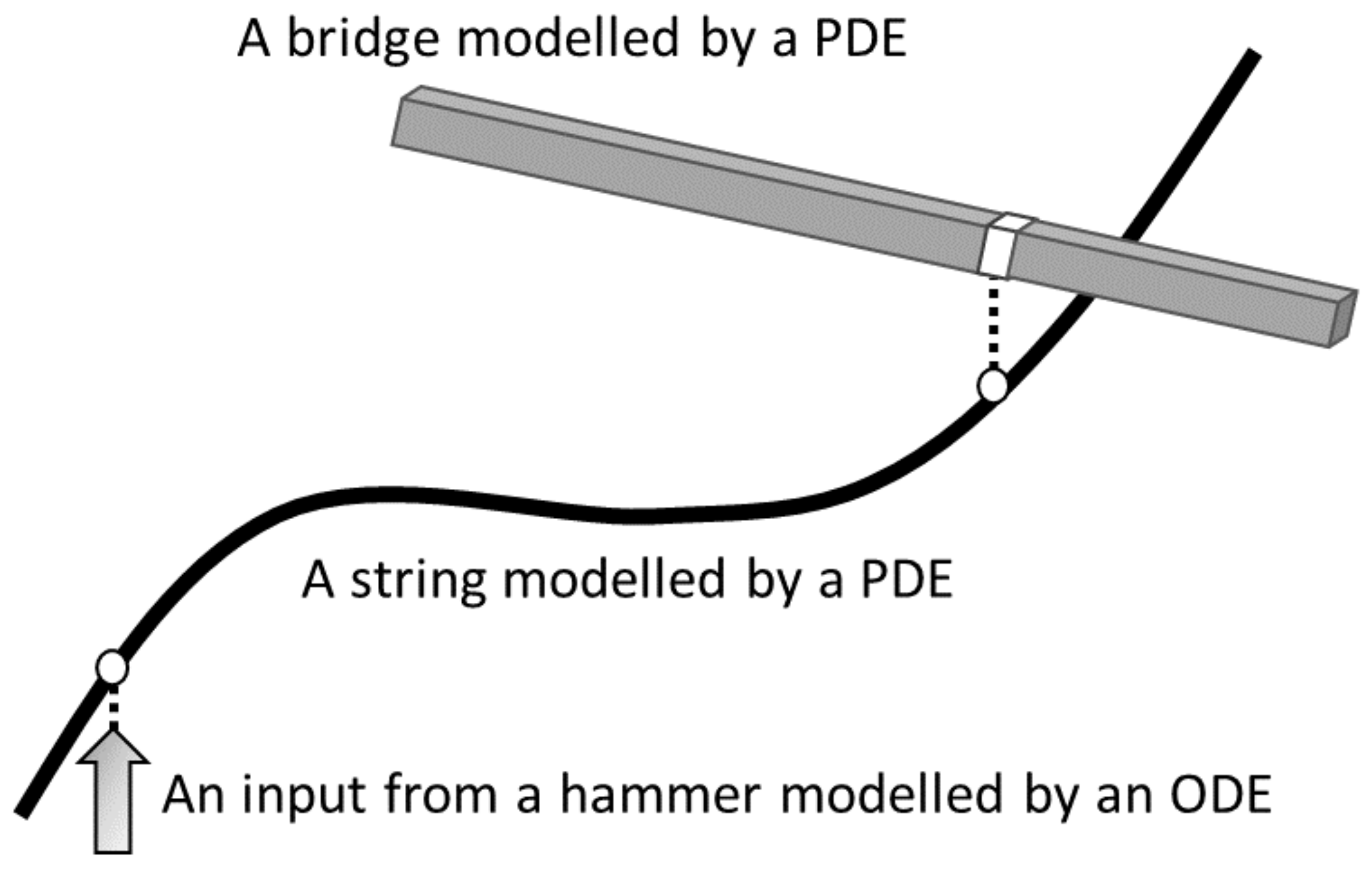
Remark 1.

The above three types of coupled systems often appear in industrial simulations. For example, let us consider simulations of the stringed musical instruments, such as the guitar and the piano [9]. The one side of strings of these instruments are typically attached to a bar-shaped part of the instruments, which is called the bridge. Each string and the bar are modeled as infinite-dimensional natural systems and they are in contact at a single point. Hence, this case corresponds to the interaction between two PDEs. Meanwhile, the strings of the piano are excited by the hammer, which is modeled as the interaction between a wave-type PDE (a model of each string) and a mass–spring ODE (a model for the hammer) (see Figure 1). In addition, designing numerical schemes for the above two cases often reduces to the case of interconnections between two ODEs by semi-discretization in space (cf. Section 4).

Figure 1. An example of coupled systems (a rough model of a piano). In this example, the string and the bridge are modeled as PDEs, which they are in contact at a single point. Excitation of the string by a hammer is typically modeled as an ODE.

2. Interconnection of Natural Systems

In this paper, we consider interconnection of two natural systems with dissipation terms. Natural systems are systems derived from the standard Lagrangian that is defined as the difference between the kinetic energy and the potential energy. For example,

$$\begin{array}{c}\hfill m\frac{{\mathrm{d}}^{2}u}{\mathrm{d}{t}^2}=-\nabla V\left(u\right),\end{array}$$

(5)

where m is a constant, u is the vector of the state variables, and V is the potential function, is a natural system because this is the Euler–Lagrange equation associated with the Lagrangian

$$\begin{array}{c}\hfill \mathcal{L}(u,\dot{u})=\frac{m}{2}\left(\frac{\mathrm{d}u}{\mathrm{d}t}·\frac{\mathrm{d}u}{\mathrm{d}t}\right)-V\left(u\right).\end{array}$$

(6)

The system in Equation (5) often arises with the damping term

$$\begin{array}{c}\hfill m\frac{{\mathrm{d}}^{2}u}{\mathrm{d}{t}^2}=-\nabla V\left(u\right)-𝒢\frac{\mathrm{d}u}{\mathrm{d}t},\end{array}$$

(7)

in which $𝒢$ is a positive semidefinite operator. If $𝒢$ is proportional to the identity operator, the operator $𝒢$ essentially denotes the damping coefficient. For simplicity of notation, regarding $𝒢$ as a 2-form, we often write for vectors or functions $w_1$ and $w_2$

$$\begin{array}{c}\hfill 𝒢(w_1,w_2)=w_1^{\top }𝒢w_2\end{array}$$

(8)

or

$$\begin{array}{c}\hfill 𝒢(w_1,w_2)=\int w_1𝒢w_2\mathrm{d}x.\end{array}$$

(9)

These are nonnegative if $w_1=w_2$.

Another example of a natural system is the Euler–Lagrange partial differential equation of the following form:

$$\begin{array}{c}\hfill \rho \frac{{\partial }^{2}u}{\partial t^2}=-\frac{\delta H}{\delta u},\end{array}$$

(10)

where $\rho$ is typically the density and $\delta H/\delta u$ the variational derivative. The variational derivative is the gradient in functional spaces, which is defined by the function that satisfies

$$\begin{array}{c}\hfill \mathrm{d}H\left(\delta u\right)={⟨\frac{\delta H}{\delta u},\delta u⟩}_{L^2}.\end{array}$$

(11)

$\mathrm{d}H$ is the Fréchet derivative and ${⟨·,·⟩}_{L^2}$ is the standard $L^2$ inner product. In fact, the partial differential Equation (10) has the Lagrangian

$$\begin{array}{c}\hfill \mathcal{L}(u,\frac{\partial u}{\partial t})=\int \left[\frac{\rho }{2}{\left(\frac{\partial u}{\partial t}\right)}^2-H\left(u\right)\right]\mathrm{d}x.\end{array}$$

(12)

Similar to Equation (5), Equation (10) is often accompanied by dissipation terms:

$$\begin{array}{c}\hfill \rho \frac{{\partial }^{2}u}{\partial t^2}=-\frac{\delta H}{\delta u}-𝒢\frac{\partial u}{\partial t}.\end{array}$$

(13)

Example 1.

For example, the wave equation

$$\begin{array}{c}\hfill \frac{{\partial }^{2}u}{\partial t^2}=c^2\frac{{\partial }^{2}u}{\partial x^2}\end{array}$$

(14)

on the interval $(0,L)$ under the periodic boundary condition is the Euler–Lagrange partial differential equation, of which Lagrangian is

$$\begin{array}{c}\hfill {\int }_0^L\left[\rho {\left(\frac{\partial u}{\partial t}\right)}^2-\frac{c^2}{2}{\left(\frac{\partial u}{\partial x}\right)}^2\right]\mathrm{d}x.\end{array}$$

(15)

In this example, H is

$$\begin{array}{c}\hfill H\left(u\right)={\int }_0^L\frac{c^2}{2}{\left(\frac{\partial u}{\partial x}\right)}^2\mathrm{d}x\end{array}$$

(16)

and the variational derivative of this functional is

$$\begin{array}{c}\hfill \frac{\delta H}{\delta u}=-c^2\frac{{\partial }^{2}u}{\partial x^2}\end{array}$$

(17)

because under the periodic boundary condition it follows that

$$\begin{array}{c}\hfill \mathrm{d}H\left(\delta u\right)={\int }_0^L\left(-c^2\frac{{\partial }^{2}u}{\partial x^2}\right)\delta u\mathrm{d}x={⟨-c^2\frac{{\partial }^{2}u}{\partial x^2},\delta u⟩}_{L^2}\end{array}$$

(18)

from the formal calculation

$$\begin{array}{cc}H(u+\delta u)-H\left(u\right)& ={\int }_0^L\frac{c^2}{2}{\left(\frac{\partial }{\partial x}(u+\delta u)\right)}^2\mathrm{d}x-{\int }_0^L{c}^2{\left(\frac{\partial u}{\partial x}\right)}^2\mathrm{d}x\\ & ={\int }_0^L{c}^2\frac{\partial u}{\partial x}\frac{\partial \delta u}{\partial x}\mathrm{d}x+(higher order terms)\\ & ={\int }_0^L\left(-c^2\frac{{\partial }^{2}u}{\partial x^2}\delta u\right)\mathrm{d}x+(higher order terms.)\end{array}$$

(19)

Throughout this paper, we suppose that two natural systems with dissipation terms of the form in Equation (7) or Equation (13) are in contact at a single point and through this point the two systems are exerting a force on each other. As noted in the Introduction, we consider the following three cases: interconnections between an ODE and an ODE, a PDE and a PDE, and an ODE and a PDE.

To begin with, we consider the first case. As mentioned above, we assume that systems are interconnected in such a way that the force between each two subsystems is described by the action—reaction law. More specifically, we assume that the coupled model is written in the form

$$\begin{array}{c}\hfill m_1\frac{{\mathrm{d}}^2{u}_1}{\mathrm{d}{t}^2}=-\nabla V_1\left(u_1\right)-{𝒢}_1\frac{\mathrm{d}{u}_1}{\mathrm{d}t}+f{e}_i,m_2\frac{{\mathrm{d}}^2{u}_2}{\mathrm{d}{t}^2}=-\nabla V_2\left(u_2\right)-{𝒢}_2\frac{\mathrm{d}{u}_2}{\mathrm{d}t}-f{e}_j.\end{array}$$

(20)

$u_1\in {\mathbb{R}}^{n_1},u_2\in {\mathbb{R}}^{n_2}$ are vectors of state variables which are possibly of different dimensions. $e_j$ is the jth unit vector representing the contact point. f is the scalar function of t, which we define so that the total energy of this system is preserved when the dissipation terms do not exist. First, the time derivative of the total energy of the system is

$$\begin{array}{c}\frac{\mathrm{d}}{\mathrm{d}t}\left(\frac{m_1}{2}\left(\frac{\mathrm{d}{u}_1}{\mathrm{d}t}·\frac{\mathrm{d}{u}_1}{\mathrm{d}t}\right)+V_1\left(u_1\right)+\frac{m_2}{2}\left(\frac{\mathrm{d}{u}_1}{\mathrm{d}t}·\frac{\mathrm{d}{u}_1}{\mathrm{d}t}\right)+V_2\left(u_2\right)\right)\\ =m_1\left(\frac{{\mathrm{d}u}_1}{\mathrm{d}t}·\frac{{\mathrm{d}}^2{u}_1}{\mathrm{d}{t}^2}\right)+\frac{{\mathrm{d}u}_1}{\mathrm{d}t}·\nabla V_1\left(u_1\right)+m_2\left(\frac{{\mathrm{d}u}_2}{\mathrm{d}t}·\frac{{\mathrm{d}}^2{u}_2}{\mathrm{d}{t}^2}\right)+\frac{{\mathrm{d}u}_2}{\mathrm{d}t}·\nabla V_2\left(u_2\right).\end{array}$$

(21)

Substitution of the equation yields

$$\begin{array}{cc}Equation\left(21\right)\hfill & =\frac{\mathrm{d}{u}_1}{\mathrm{d}t}·\left(-\nabla V_1\left(u_1\right)-{𝒢}_1\frac{\mathrm{d}{u}_1}{\mathrm{d}t}+f{e}_i\right)+\frac{\mathrm{d}{u}_1}{\mathrm{d}t}·\nabla V_1\left(u_1\right)\hfill \\ & +\frac{\mathrm{d}{u}_2}{\mathrm{d}t}·\left(-\nabla V_2\left(u_2\right)-{𝒢}_2\frac{\mathrm{d}{u}_2}{\mathrm{d}t}-f{e}_j\right)+\frac{\mathrm{d}{u}_2}{\mathrm{d}t}·\nabla V_2\left(u_2\right)\hfill \\ & =-{𝒢}_1(\frac{\mathrm{d}{u}_1}{\mathrm{d}t},\frac{\mathrm{d}{u}_1}{\mathrm{d}t})-{𝒢}_2(\frac{\mathrm{d}{u}_2}{\mathrm{d}t},\frac{\mathrm{d}{u}_2}{\mathrm{d}t})+f\frac{\mathrm{d}{u}_1}{\mathrm{d}t}·e_i-f\frac{\mathrm{d}{u}_2}{\mathrm{d}t}·e_j\hfill \\ & =-{𝒢}_1(\frac{\mathrm{d}{u}_1}{\mathrm{d}t},\frac{\mathrm{d}{u}_1}{\mathrm{d}t})-{𝒢}_2(\frac{\mathrm{d}{u}_2}{\mathrm{d}t},\frac{\mathrm{d}{u}_2}{\mathrm{d}t})+f\left[{\left(\frac{\mathrm{d}{u}_1}{\mathrm{d}t}\right)}_i-{\left(\frac{\mathrm{d}{u}_2}{\mathrm{d}t}\right)}_j\right],\hfill \end{array}$$

(22)

where ${\left(\frac{\mathrm{d}{u}_k}{\mathrm{d}t}\right)}_i$ denotes the ith component of the vector $\frac{\mathrm{d}{u}_k}{\mathrm{d}t}$. In the absence of the dissipation terms, this becomes

$$\begin{array}{c}\hfill f\left[{\left(\frac{\mathrm{d}{u}_1}{\mathrm{d}t}\right)}_i-{\left(\frac{\mathrm{d}{u}_2}{\mathrm{d}t}\right)}_j\right].\end{array}$$

(23)

Thus, for conservation of the energy

$$\begin{array}{c}\hfill {\left(\frac{\mathrm{d}{u}_1}{\mathrm{d}t}\right)}_i={\left(\frac{\mathrm{d}{u}_2}{\mathrm{d}t}\right)}_j\end{array}$$

(24)

is sufficient. For this condition to be held, we impose that

$$\begin{array}{c}\hfill {\left(\frac{{\mathrm{d}}^2{u}_1}{\mathrm{d}{t}^2}\right)}_i={\left(\frac{{\mathrm{d}}^2{u}_2}{\mathrm{d}{t}^2}\right)}_j,{\left.{\left(\frac{\mathrm{d}{u}_1}{\mathrm{d}t}\right)}_i\right|}_{t=0}={\left.{\left(\frac{\mathrm{d}{u}_2}{\mathrm{d}t}\right)}_j\right|}_{t=0}\end{array}$$

(25)

also for the systems with dissipation terms. From Equation (20) and the first equality of Equation (25), we get

$$\begin{array}{c}\hfill \frac{1}{m_1}\left[-{\left(\nabla V_1\left(u_1\right)\right)}_i-{𝒢}_1{\left(\frac{\mathrm{d}{u}_1}{\mathrm{d}t}\right)}_i+f\right]=\frac{1}{m_2}\left[-{\left(\nabla V_2\left(u_2\right)\right)}_j-{𝒢}_1{\left(\frac{\mathrm{d}{u}_2}{\mathrm{d}t}\right)}_j-f\right],\end{array}$$

(26)

which gives

$$\begin{array}{c}\hfill f=\frac{m_2}{m_1+m_2}{(\nabla V_1\left(u_1\right)-{𝒢}_1\frac{\mathrm{d}{u}_1}{\mathrm{d}t})}_i-\frac{m_1}{m_1+m_2}{(\nabla V_2\left(u_2\right)-{𝒢}_1\frac{\mathrm{d}{u}_2}{\mathrm{d}t})}_j.\end{array}$$

(27)

As a result, the coupled model equation is

$$\begin{array}{cc}\hfill & m_1\frac{{\mathrm{d}}^2{u}_1}{\mathrm{d}{t}^2}=-\nabla V_1\left(u_1\right)-{𝒢}_1\frac{\mathrm{d}{u}_1}{\mathrm{d}t}+f{e}_i,m_2\frac{{\mathrm{d}}^2{u}_2}{\mathrm{d}{t}^2}=-\nabla V_2\left(u_2\right)-{𝒢}_2\frac{\mathrm{d}{u}_2}{\mathrm{d}t}-f{e}_j,\hfill \end{array}$$

$$\begin{array}{c}\hfill f=\frac{m_2}{m_1+m_2}{(\nabla V_1\left(u_1\right)-{𝒢}_1\frac{\mathrm{d}{u}_1}{\mathrm{d}t})}_i-\frac{m_1}{m_1+m_2}{(\nabla V_2\left(u_2\right)-{𝒢}_2\frac{\mathrm{d}{u}_2}{\mathrm{d}t})}_j.\end{array}$$

(28)

Remark 2.

If we write

$$\begin{array}{c}{q}_1=u_1,p_1=m_1\frac{\mathrm{d}{u}_1}{\mathrm{d}t},q_2=u_2,p_2=m_2\frac{\mathrm{d}{u}_2}{\mathrm{d}t},\hfill \\ H(q_1,p_1,q_2,p_2)=\frac{1}{2m_1}{p}_1·p_1+V_1\left(q_1\right)+\frac{1}{2m_2}{p}_2·p_2+V_2\left(q_2\right),\hfill \end{array}$$

(29)

Equation (28) without the dissipation terms can be written in the Hamiltonian formalism:

$$\begin{array}{ll}\frac{\mathrm{d}}{\mathrm{d}t}\left(\begin{array}{c}{q}_1\\ p_1\\ q_2\\ p_2\end{array}\right)\hfill & =\left(\begin{array}{cccc}O& I& O& O\\ -I& O& O& O\\ O& O& O& I\\ O& O& -I& O\end{array}\right)\left(\begin{array}{c}\nabla V_1\left(q_1\right)\\ {\displaystyle \frac{p_1}{m_1}}\\ \nabla V_2\left(q_2\right)\\ {\displaystyle \frac{p_2}{m_2}}\end{array}\right)\\ & +\left(\begin{array}{c}0\\ \left\{\begin{array}{cc}\frac{1}{m_1+m_2}\left(m_2{(\nabla V_1\left(q_1\right))}_i-m_1{(\nabla V_2\left(q_2\right))}_j\right)\hfill & \left((n_1+i)\mathrm{th} \mathrm{component}\right)\hfill \\ 0\hfill & \left(\mathrm{otherwise}\right)\hfill \end{array}\right.\\ 0\\ \left\{\begin{array}{cc}-\frac{1}{m_1+m_2}\left(m_2{(\nabla V_1\left(q_1\right))}_i-m_1{(\nabla V_2\left(q_2\right))}_j\right)\hfill & ((2n_1+n_2+j)\mathrm{th} \mathrm{component}\hfill \\ 0\hfill & \left(\mathrm{otherwise}\right)\hfill \end{array}\right.\end{array}\right)\\ & =\left(\begin{array}{cccc}O& I& O& O\\ -I& O& O& O\\ O& O& O& I\\ O& O& -I& O\end{array}\right)\left(\begin{array}{c}{\displaystyle \frac{\partial H}{\partial q_1}}\\ {\displaystyle \frac{\partial H}{\partial p_1}}\\ {\displaystyle \frac{\partial H}{\partial q_2}}\\ {\displaystyle \frac{\partial H}{\partial p_2}}\end{array}\right)\\ & +\left(\begin{array}{c}0\\ \left\{\begin{array}{cc}\frac{1}{m_1+m_2}\left(m_2{\left(\frac{\partial H}{\partial q_1}\right)}_i-m_1{\left(\frac{\partial H}{\partial q_2}\right)}_j\right)\hfill & \left((n_1+i)\mathrm{th} \mathrm{component}\right)\hfill \\ 0\hfill & \left(\mathrm{otherwise}\right)\hfill \end{array}\right.\\ 0\\ \left\{\begin{array}{cc}-\frac{1}{m_1+m_2}\left(m_2{\left(\frac{\partial H}{\partial q_1}\right)}_i-m_1{\left(\frac{\partial H}{\partial q_2}\right)}_j\right)\hfill & \left((2n_1+n_2+j)\mathrm{th} \mathrm{component}\right)\hfill \\ 0\hfill & \left(\mathrm{otherwise}\right)\hfill \end{array}\right.\end{array}\right)\\ & =\left[\left(\begin{array}{cccc}O& I& O& O\\ -I& O& O& O\\ O& O& O& I\\ O& O& -I& O\end{array}\right)+B\right]\left(\begin{array}{c}{\displaystyle \frac{\partial H}{\partial q_1}}\\ {\displaystyle \frac{\partial H}{\partial p_1}}\\ {\displaystyle \frac{\partial H}{\partial q_2}}\\ {\displaystyle \frac{\partial H}{\partial p_2}}\end{array}\right),\hfill \end{array}$$

(30)

where B is the matrix that has only 4 non-zero components

$$\begin{array}{cc}\hfill & B_{i+n_1,i}=\frac{m_2}{m_1+m_2},B_{i+n_1,j+2n_1}=-\frac{m_1}{m_1+m_2},\hfill \\ \hfill & B_{j+2n_1+n_2,i}=-\frac{m_2}{m_1+m_2},B_{j+2n_1+n_2,j+2n_1}=\frac{m_1}{m_1+m_2}.\hfill \end{array}$$

(31)

Because, unfortunately, the matrix B is not skew-symmetric, the equation is not of the form in Equation (4); however, as shown in the next theorem, the total energy is conserved.

Theorem 1.

Provided that

$$\begin{array}{c}\hfill {\left.{\left(\frac{\mathrm{d}{u}_1}{\mathrm{d}t}\right)}_i\right|}_{t=0}={\left.{\left(\frac{\mathrm{d}{u}_2}{\mathrm{d}t}\right)}_j\right|}_{t=0},\end{array}$$

(32)

for any solutions to the equations of the interconnected systems

$$\begin{array}{cc}\hfill & m_1\frac{{\mathrm{d}}^2{u}_1}{\mathrm{d}{t}^2}=-\nabla V_1\left(u_1\right)-{𝒢}_1\frac{\mathrm{d}{u}_1}{\mathrm{d}t}+f{e}_i,m_2\frac{{\mathrm{d}}^2{u}_2}{\mathrm{d}{t}^2}=-\nabla V_2\left(u_2\right)-{𝒢}_2\frac{\mathrm{d}{u}_2}{\mathrm{d}t}-f{e}_j,\hfill \end{array}$$

(33)

$$f=\frac{m_2}{m_1+m_2}(\nabla V_1\left(u_1\right)+{𝒢}_1\frac{\mathrm{d}{u}_1}{\mathrm{d}t}{)}_i-\frac{m_1}{m_1+m_2}(\nabla V_2\left(u_2\right)+{𝒢}_2\frac{\mathrm{d}{u}_2}{\mathrm{d}t}{)}_j,$$

(34)

the energy is not increasing:

$$\begin{array}{c}\frac{\mathrm{d}E}{\mathrm{d}t}=-{𝒢}_1(\frac{\mathrm{d}{u}_1}{\mathrm{d}t},\frac{\mathrm{d}{u}_1}{\mathrm{d}t})-{𝒢}_2(\frac{\mathrm{d}{u}_2}{\mathrm{d}t},\frac{\mathrm{d}{u}_2}{\mathrm{d}t})\le 0,\hfill \\ E=E_1+E_2,E_1=\frac{m_1}{2}\left(\frac{\mathrm{d}{u}_1}{\mathrm{d}t}·\frac{\mathrm{d}{u}_1}{\mathrm{d}t}\right)+V\left(u_1\right),E_2=\frac{m_2}{2}\left(\frac{\mathrm{d}{u}_2}{\mathrm{d}t}·\frac{\mathrm{d}{u}_2}{\mathrm{d}t}\right)+V\left(u_2\right).\hfill \end{array}$$

(35)

In particular, in the absence of the dissipation terms, that is, ${}_1{=}_2=0$, the energy is preserved:

$$\begin{array}{c}\hfill \frac{\mathrm{d}E}{\mathrm{d}t}=0.\end{array}$$

(36)

Proof. 

From ith and jth elements of Equation (33), the following equations hold:

$$\begin{array}{cc}\hfill & m_1{\left.\left(\frac{{\mathrm{d}}^2{u}_1}{\mathrm{d}{t}^2}\right)\right|}_i=-{\left(\nabla V_1\left(u_1\right)+{𝒢}_1\frac{\mathrm{d}{u}_1}{\mathrm{d}t}\right)}_i+f,m_2{\left.\left(\frac{{\mathrm{d}}^2{u}_2}{\mathrm{d}{t}^2}\right)\right|}_j=-{\left(\nabla V_2\left(u_2\right)+{𝒢}_2\frac{\mathrm{d}{u}_2}{\mathrm{d}t}\right)}_j-f.\hfill \end{array}$$

Substitution of Equation (34) into the above yields

$$\begin{array}{cc}\hfill & m_1{\left.\left(\frac{{\mathrm{d}}^2{u}_1}{\mathrm{d}{t}^2}\right)\right|}_i\hfill \\ \hfill & =-{\left(\nabla V_1\left(u_1\right)+{𝒢}_1\frac{\mathrm{d}{u}_1}{\mathrm{d}t}\right)}_i+\frac{m_2}{m_1+m_2}{\left(\nabla V_1\left(u_1\right)+{𝒢}_1\frac{\mathrm{d}{u}_1}{\mathrm{d}t}\right)}_i-\frac{m_1}{m_1+m_2}{\left(\nabla V_2\left(u_2\right)+{𝒢}_2\frac{\mathrm{d}{u}_2}{\mathrm{d}t}\right)}_j\hfill \\ \hfill & =-\frac{m_1}{m_1+m_2}{\left(\nabla V_1\left(u_1\right)+{𝒢}_1\frac{\mathrm{d}{u}_1}{\mathrm{d}t}\right)}_i-\frac{m_1}{m_1+m_2}{\left(\nabla V_2\left(u_2\right)+{𝒢}_2\frac{\mathrm{d}{u}_2}{\mathrm{d}t}\right)}_j,\hfill \end{array}$$

which is equivalent to

$$\begin{array}{cc}\hfill & {\left.\left(\frac{{\mathrm{d}}^2{u}_1}{\mathrm{d}{t}^2}\right)\right|}_i=-\frac{1}{m_1+m_2}{\left(\nabla V_1\left(u_1\right)+{𝒢}_1\frac{\mathrm{d}{u}_1}{\mathrm{d}t}\right)}_i-\frac{1}{m_1+m_2}{\left(\nabla V_2\left(u_2\right)+{𝒢}_2\frac{\mathrm{d}{u}_2}{\mathrm{d}t}\right)}_j.\hfill \end{array}$$

In the same way, we have

$$\begin{array}{cc}\hfill & m_2{\left.\left(\frac{{\mathrm{d}}^2{u}_2}{\mathrm{d}{t}^2}\right)\right|}_j=-\frac{m_2}{m_1+m_2}{\left(\nabla V_1\left(u_1\right)+{𝒢}_1\frac{\mathrm{d}{u}_1}{\mathrm{d}t}\right)}_i+\frac{m_2}{m_1+m_2}{\left(\nabla V_2\left(u_2\right)+{𝒢}_2\frac{\mathrm{d}{u}_2}{\mathrm{d}t}\right)}_j\hfill \end{array}$$

and, hence,

$$\begin{array}{cc}\hfill & {\left.\left(\frac{{\mathrm{d}}^2{u}_2}{\mathrm{d}{t}^2}\right)\right|}_j=-\frac{1}{m_1+m_2}{\left(\nabla V_1\left(u_1\right)+{𝒢}_1\frac{\mathrm{d}{u}_1}{\mathrm{d}t}\right)}_i-\frac{1}{m_1+m_2}{\left(\nabla V_2\left(u_2\right)+{𝒢}_2\frac{\mathrm{d}{u}_2}{\mathrm{d}t}\right)}_j.\hfill \end{array}$$

Thus, we get

$$\begin{array}{c}\hfill {\left(\frac{{\mathrm{d}}^2{u}_1}{\mathrm{d}{t}^2}\right)}_i={\left(\frac{{\mathrm{d}}^2{u}_2}{\mathrm{d}{t}^2}\right)}_j\end{array}$$

(37)

for all t. Hence, using the assumption on the initial conditions in Equation (32), for any t, we have

$$\begin{array}{c}\hfill {\left(\frac{\mathrm{d}{u}_1}{\mathrm{d}t}\right)}_i={\left(\frac{\mathrm{d}{u}_2}{\mathrm{d}t}\right)}_j.\end{array}$$

(38)

Meanwhile, as shown in Equation (22), the time derivative of the energy is computed as below:

$$\begin{array}{cc}\hfill & \frac{\mathrm{d}E}{\mathrm{d}t}=-{𝒢}_1(\frac{\mathrm{d}{u}_1}{\mathrm{d}t},\frac{\mathrm{d}{u}_1}{\mathrm{d}t})-{𝒢}_2(\frac{\mathrm{d}{u}_2}{\mathrm{d}t},\frac{\mathrm{d}{u}_2}{\mathrm{d}t})+f\left[{\left(\frac{\mathrm{d}{u}_1}{\mathrm{d}t}\right)}_i-{\left(\frac{\mathrm{d}{u}_2}{\mathrm{d}t}\right)}_j\right].\hfill \end{array}$$

Therefore, from Equation (38), we obtain

$$\begin{array}{c}\hfill \frac{\mathrm{d}E}{\mathrm{d}t}=-{𝒢}_1(\frac{\mathrm{d}{u}_1}{\mathrm{d}t},\frac{\mathrm{d}{u}_1}{\mathrm{d}t})-{𝒢}_2(\frac{\mathrm{d}{u}_2}{\mathrm{d}t},\frac{\mathrm{d}{u}_2}{\mathrm{d}t}).\end{array}$$

(39)

□

In the same way, we can obtain similar theorems for the other two types of the interconnected systems. Firstly, we consider

$$\begin{array}{c}\hfill {\rho }_1\frac{{\partial }^2{u}_1}{\partial t^2}=-\frac{\delta V_1}{\delta u_1}-{𝒢}_1\frac{\partial u_1}{\partial t}+f\delta (x-x_1)x_1\in (0,L_1),\\ \hfill {\rho }_2\frac{{\partial }^2{u}_2}{\partial t^2}=-\frac{\delta V_2}{\delta u_2}-{𝒢}_2\frac{\partial u_2}{\partial t}-f\delta (x-x_2)x_2\in (0,L_2),\end{array}$$

(40)

where f is a scalar function of t. $\delta$ is the Dirac delta function, and hence the equalities in the above equations are in the weak sense; however, the following computations are naively performed for simplicity. The terms with the Delta function represent that the two systems are interconnected at $x=x_1$ for the first system and $x=x_2$ for the second. For this coupled system, the total energy is defined by

$$\begin{array}{cc}\hfill & E=E_1+E_2,\hfill \\ \hfill & E_1={\int }_0^{L_1}\left[\frac{{\rho }_1}{2}{\left(\frac{\partial u_1}{\partial t}\right)}^2+V_1\left(u\right)\right]\mathrm{d}x,E_2={\int }_0^{L_2}\left[\frac{{\rho }_2}{2}{\left(\frac{\partial u_2}{\partial t}\right)}^2+V_2\left(u_2\right)\right]\mathrm{d}x.\hfill \end{array}$$

(41)

Theorem 2.

Suppose that the boundary condition is appropriately imposed so that

$$\begin{array}{cc}\hfill \frac{\mathrm{d}E}{\mathrm{d}t}=& {\int }_0^{L_1}\frac{\partial u_1}{\partial t}\left({\rho }_1\frac{{\partial }^2{u}_1}{\partial t^2}+\frac{\delta V_1}{\delta u_1}\right)\mathrm{d}x+{\int }_0^{L_2}\frac{\partial u_2}{\partial t}\left({\rho }_2\frac{{\partial }^2{u}_2}{\partial t^2}+\frac{\delta V_2}{\delta u_2}\right)\mathrm{d}x.\hfill \end{array}$$

(42)

Provided that

$$\begin{array}{c}\hfill {\left.{\left(\frac{\partial u_1}{\partial t}\right)}_{x=x_1}\right|}_{t=0}={\left.{\left(\frac{\partial u_2}{\partial t}\right)}_{x=x_2}\right|}_{t=0},\end{array}$$

(43)

for any solutions to the equations of the interconnected systems

$$\begin{array}{cc}\hfill & {\rho }_1\frac{{\partial }^2{u}_1}{\partial t^2}=-\frac{\delta V_1}{\delta u_1}-{𝒢}_1\frac{\partial u_1}{\partial t}+f\delta (x-x_1),{\rho }_2\frac{{\partial }^2{u}_2}{\partial t^2}=-\frac{\delta V_2}{\delta u_2}-{𝒢}_2\frac{\partial u_2}{\partial t}-f\delta (x-x_2),\hfill \\ \hfill & f=\frac{{\rho }_2}{{\rho }_1+{\rho }_2}{\left(\frac{\delta V_1}{\delta u_1}+{𝒢}_1\frac{\partial u_1}{\partial t}\right)}_{x=x_1}-\frac{{\rho }_1}{{\rho }_1+{\rho }_2}{\left(\frac{\delta V_2}{\delta u_2}+{𝒢}_2\frac{\partial u_2}{\partial t}\right)}_{x=x_2}\hfill \end{array}$$

(44)

the energy is not increasing:

$$\begin{array}{c}\hfill \frac{\mathrm{d}E}{\mathrm{d}t}=-{\int }_0^{L_1}{𝒢}_1(\frac{\partial u_1}{\partial t},\frac{\partial u_1}{\partial t})\mathrm{d}x-{\int }_0^{L_2}{𝒢}_2(\frac{\partial u_2}{\partial t},\frac{\partial u_2}{\partial t})\mathrm{d}x\le 0.\end{array}$$

(45)

In particular, in the absence of the dissipation terms, the energy is preserved:

$$\begin{array}{c}\hfill \frac{\mathrm{d}E}{\mathrm{d}t}=0.\end{array}$$

(46)

Secondly, we consider

$$\begin{array}{c}\hfill m\frac{{\mathrm{d}}^2{u}_1}{\mathrm{d}{t}^2}=-\nabla V_1\left(u_1\right)-{𝒢}_1\frac{\mathrm{d}{u}_1}{\mathrm{d}t}+f{e}_i,\rho \frac{{\partial }^2{u}_2}{\partial t^2}=-\frac{\delta V_2}{\delta u_2}-{𝒢}_2\frac{\partial u_2}{\partial t}-f\delta (x-x_2)(x\in (0,L_2)),\end{array}$$

(47)

of which the total energy is

$$\begin{array}{cc}\hfill & E=E_1+E_2,\hfill \\ \hfill & E_1=\frac{m}{2}\frac{\mathrm{d}{u}_1}{\mathrm{d}t}·\frac{\mathrm{d}{u}_1}{\mathrm{d}t}+V_1\left(u_1\right),E_2={\int }_0^{L_2}\left[\frac{\rho }{2}{\left(\frac{\partial u_2}{\partial t}\right)}^2+V_2\left(u_2\right)\right]\mathrm{d}x.\hfill \end{array}$$

(48)

Theorem 3.

Suppose that the boundary condition is appropriately given so that

$$\begin{array}{c}\hfill \frac{\mathrm{d}E}{\mathrm{d}t}=\frac{\mathrm{d}{u}_1}{\mathrm{d}t}·\left(m\frac{{\mathrm{d}}^2{u}_1}{\mathrm{d}{t}^2}+\nabla V_1\left(u_1\right)\right)+{\int }_0^{L_2}\frac{\partial u_2}{\partial t}·\left(\rho \frac{{\partial }^2{u}_2}{\partial t^2}+\frac{\delta V_2}{\delta u_2}\right)\mathrm{d}x.\end{array}$$

(49)

Provided that

$$\begin{array}{c}\hfill {\left.{\left(\frac{\mathrm{d}{u}_1}{\mathrm{d}t}\right)}_i\right|}_{t=0}={\left.{\left(\frac{\partial u_2}{\partial t}\right)}_{x=x_2}\right|}_{t=0},\end{array}$$

(50)

for any solutions to the equations of the interconnected systems

$$\begin{array}{c}m\frac{{\mathrm{d}}^2{u}_1}{\mathrm{d}{t}^2}=-\nabla V_1\left(u_1\right){-}_1\frac{\mathrm{d}{u}_1}{\mathrm{d}t}+f{e}_i,\rho \frac{{\partial }^2{u}_2}{\partial t^2}=-\frac{\delta V_2}{\delta u_2}{-}_2\frac{\partial u_2}{\partial t}-f\delta (x-x_2),\hfill \\ f=\frac{\rho }{m+\rho }{(\nabla V_1{+}_1\frac{\mathrm{d}{u}_1}{\mathrm{d}t})}_i-\frac{m}{m+\rho }{\left(\frac{\delta V_2}{\delta u_2}{+}_2\frac{\partial u_2}{\partial t}\right)}_{x=x_2}\hfill \end{array}$$

(51)

the energy is not increasing:

$$\begin{array}{cc}\hfill & \frac{\mathrm{d}E}{\mathrm{d}t}=-{𝒢}_1(\frac{\mathrm{d}{u}_1}{\mathrm{d}t},\frac{\mathrm{d}{u}_1}{\mathrm{d}t})-{\int }_0^{L_2}{𝒢}_2(\frac{\partial u_2}{\partial t},\frac{\partial u_2}{\partial t})\mathrm{d}x\le 0.\hfill \end{array}$$

(52)

In particular, in the absence of the dissipation terms, the energy is preserved:

$$\begin{array}{c}\hfill \frac{\mathrm{d}E}{\mathrm{d}t}=0.\end{array}$$

(53)

We omit the proofs of Theorems 2 and 3 because they are proved exactly in the same way as Theorem 1.

3. Energetic-Property-Preserving Numerical Schemes for the Finite Dimensional Coupled Systems

In this section, we propose energetic-property-preserving numerical schemes for the above finite-dimensional coupled systems. Although the equation is not of the form in Equation (4), we use the discrete gradient similarly to CelledoniHøiseth [8]. A discrete gradient is defined as follows (see, e.g., [10])

Definition 1.

A discrete gradient of a function $V:{\mathbb{R}}^N\to \mathbb{R}$ is defined by a vector valued function $\overline{\nabla }V(u,v)$ such that

$$\begin{array}{c}\hfill V\left(u\right)-V\left(v\right)=\overline{\nabla }V(u,v)·(u-v),\overline{\nabla }V(u,u)=\nabla V\left(u\right).\end{array}$$

(54)

The first condition is a discrete counterpart of the chain rule

$$\begin{array}{c}\hfill \frac{\mathrm{d}V}{\mathrm{d}t}=\nabla V·\frac{\mathrm{d}u}{\mathrm{d}t}.\end{array}$$

(55)

The second condition assures that a discrete gradient is indeed an approximation of the gradient. A discrete gradient is not uniquely determined and hence several ways for designing a discrete gradient have been proposed. A typical way is the average vector field method [11]:

$$\begin{array}{c}\hfill \overline{\nabla }V(u,v)={\int }_0^1\nabla V((1-s)u+sv)\mathrm{d}s.\end{array}$$

(56)

Another choice for obtaining a discrete gradient is the automatic discrete differentiation, which is a method to automatically derive a discrete gradient in a similar way to the automatic differentiation; see [12].

In what follows, we use the following symbols for the discrete systems. The step sizes are denoted, for example, by $\Delta t$ and $\Delta x$. An approximation of $u(n\Delta t)$ is denoted by $u^{\left(n\right)}$, where $u^{\left(n\right)}$ can be a vector $u^{\left(n\right)}={(u_1^{\left(n\right)},\dots ,u_N^{\left(n\right)})}^{\top }$. Similarly, for partial differential equations, an approximation of $u(n\Delta t,j\Delta x)$ is denoted by $u_j^{\left(n\right)}$. For simplicity of notation, we also use the following difference operators:

$$\begin{array}{cc}\hfill & {\delta }_t^{+}{u}_j^{\left(n\right)}:=\frac{u_j^{(n+1)}-u_j^{\left(n\right)}}{\Delta t},{\delta }_t^{-}{u}_j^{\left(n\right)}:=\frac{u_j^{\left(n\right)}-u_j^{(n-1)}}{\Delta t},{\delta }_t^{⟨1⟩}{u}_j^{\left(n\right)}:=\frac{u_j^{(n+1)}-u_j^{(n-1)}}{2\Delta t},\hfill \\ \hfill & {\delta }_t^{⟨2⟩}{u}_j^{\left(n\right)}:=\frac{u_j^{(n+1)}-2u_j^{\left(n\right)}+u_j^{(n-1)}}{{(\Delta t)}^2},\hfill \\ \hfill & {\delta }_x^{+}{u}_j^{\left(n\right)}:=\frac{u_{j+1}^{\left(n\right)}-u_j^{\left(n\right)}}{\Delta x},{\delta }_x^{-}{u}_j^{\left(n\right)}:=\frac{u_j^{\left(n\right)}-u_{j-1}^{\left(n\right)}}{\Delta x},{\delta }_x^{⟨1⟩}{u}_j^{\left(n\right)}:=\frac{u_{j+1}^{\left(n\right)}-u_{j-1}^{\left(n\right)}}{2\Delta x},\hfill \\ \hfill & {\delta }_x^{⟨2⟩}{u}_j^{\left(n\right)}:=\frac{u_{j+1}^{\left(n\right)}-2u_j^{\left(n\right)}+u_{j-1}^{\left(n\right)}}{{(\Delta x)}^2},\hfill \end{array}$$

(57)

and the averaging operator

$$\begin{array}{c}\hfill {\mathcal{A}}_t^{+}{u}_j^{\left(n\right)}:=\frac{u_j^{(n+1)}+u_j^{\left(n\right)}}{2}.\end{array}$$

(58)

Note that the difference operators and the averaging operator commute; for example,

$$\begin{array}{c}\hfill {\delta }_t^{+}{\mathcal{A}}_t^{+}{u}_j^{\left(n\right)}={\mathcal{A}}_t^{+}{\delta }_t^{+}{u}_j^{\left(n\right)}.\end{array}$$

(59)

We first consider the coupled system in Equation (33). For the other two types of systems, the numerical schemes are obtained by replacing the discrete gradient by the discrete variational derivative [1,13] or by discretizing the partial differential equation in space in such a way that the resultant semi-discrete scheme becomes a finite dimensional natural system; we discuss this below.

We discretize the Hamiltonian form of Equation (33)

$$\begin{array}{c}\frac{\mathrm{d}{u}_1}{\mathrm{d}t}=v_1,m_1\frac{\mathrm{d}{v}_1}{\mathrm{d}t}=-\nabla V_1\left(u_1\right)-{𝒢}_1{v}_1+f{e}_i,\hfill \\ \frac{\mathrm{d}{u}_2}{\mathrm{d}t}=v_2,m_2\frac{\mathrm{d}{v}_2}{\mathrm{d}t}=-\nabla V_2\left(u_2\right)-{𝒢}_2{v}_2-f{e}_j,\hfill \\ f=\frac{m_2}{m_1+m_2}(\nabla V_1\left(u_1\right)+{𝒢}_1\frac{\mathrm{d}{u}_1}{\mathrm{d}t}{)}_i-\frac{m_1}{m_1+m_2}(\nabla V_2\left(u_2\right)+{𝒢}_2\frac{\mathrm{d}{u}_2}{\mathrm{d}t}{)}_j,\end{array}$$

(60)

in the following way:

$$\begin{array}{c}{\delta }_t^{+}{u}_1^{\left(n\right)}={\mathcal{A}}_t^{+}{v}_1^{\left(n\right)},m_1{\delta }_t^{+}{v}_1^{\left(n\right)}=-\overline{\nabla }{V}_1(u_1^{(n+1)},u_1^{\left(n\right)})-{𝒢}_1{\mathcal{A}}_t^{+}{v}_1^{\left(n\right)}+f^{(n+\frac{1}{2})}{e}_i,\hfill \\ {\delta }_t^{+}{u}_2^{\left(n\right)}={\mathcal{A}}_t^{+}{v}_2^{\left(n\right)},m_2{\delta }_t^{+}{v}_2^{\left(n\right)}=-\overline{\nabla }{V}_2(u_2^{(n+1)},u_2^{\left(n\right)})-{𝒢}_2{\mathcal{A}}_t^{+}{v}_2^{\left(n\right)}-f^{(n+\frac{1}{2})}{e}_j,\hfill \\ f^{(n+\frac{1}{2})}=\frac{m_2}{m_1+m_2}(\overline{\nabla }{V}_1(u_1^{(n+1)},u_1^{\left(n\right)})+{𝒢}_1{\mathcal{A}}_t^{+}{v}_1^{\left(n\right)}{)}_i-\frac{m_1}{m_1+m_2}(\overline{\nabla }{V}_2(u_2^{(n+1)},u_2^{\left(n\right)})+{𝒢}_2{\mathcal{A}}_t^{+}{v}_2^{\left(n\right)}{)}_j\hfill \end{array}$$

(61)

Under an assumption that corresponds to Equation (32), this numerical scheme preserves the energetic properties of the systems in the following sense.

Theorem 4.

Provided that

$$\begin{array}{c}\hfill \frac{{\left(u_1^{\left(1\right)}\right)}_i-{\left(u_1^{\left(0\right)}\right)}_i}{\Delta t}=\frac{{\left(u_2^{\left(1\right)}\right)}_j-{\left(u_2^{\left(0\right)}\right)}_j}{\Delta t},\end{array}$$

(62)

for any solutions to the numerical scheme in Equation (61), the total energy is not increasing:

$$\begin{array}{cc}\hfill & \frac{E_{\mathrm{d}}^{(n+1)}-E_{\mathrm{d}}^{\left(n\right)}}{\Delta t}=-{𝒢}_1({\delta }_t^{+}{u}_1^{\left(n\right)},{\delta }_t^{+}{u}_1^{\left(n\right)})-{𝒢}_2({\delta }_t^{+}{u}_2^{\left(n\right)},{\delta }_t^{+}{u}_2^{\left(n\right)})\le 0,\hfill \\ \hfill & E_{\mathrm{d}}^{\left(n\right)}=\frac{m_1}{2}{v}_1^{\left(n\right)}·v_1^{\left(n\right)}+V_1\left(u_1^{\left(n\right)}\right)+\frac{m_2}{2}{v}_2^{\left(n\right)}·v_2^{\left(n\right)}+V_2\left(u_2^{\left(n\right)}\right).\hfill \end{array}$$

(63)

In particular, in the absence of the dissipation terms, that is, ${𝒢}_1={𝒢}_2=0$, the energy is preserved:

$$\begin{array}{c}\hfill \frac{E_{\mathrm{d}}^{(n+1)}-E_{\mathrm{d}}^{\left(n\right)}}{\Delta t}=0.\end{array}$$

(64)

Proof. 

The proof is almost the same as the continuous case. First, from the definition of $f^{(n+\frac{1}{2})}$, it follows that

$$\begin{array}{cc}{m}_1{\delta }_t^{⟨2⟩}{\left(u_1^{\left(n\right)}\right)}_i\hfill & =m_1{\delta }_t^{+}{\delta }_t^{-}{\left(u_1^{\left(n\right)}\right)}_i\hfill \\ & =m_1{\delta }_t^{+}{\delta }_t^{+}{\left(u_1^{(n-1)}\right)}_i\hfill \\ & =m_1{\delta }_t^{+}{\left({\mathcal{A}}_t^{+}{v}_1^{(n-1)}\right)}_i\hfill \\ & =m_1{\mathcal{A}}_t^{+}{\left({\delta }_t^{+}{v}_1^{(n-1)}\right)}_i\hfill \\ & ={\mathcal{A}}_t^{+}\left(-\overline{\nabla }{V}_1{(u_1^{\left(n\right)},u_1^{(n-1)})}_i-{𝒢}_1{\mathcal{A}}_t^{+}{v}_1^{(n-1)}+f^{(n-\frac{1}{2})}\right)\hfill \\ & ={\mathcal{A}}_t^{+}\left[-{\left(\overline{\nabla }{V}_1(u_1^{\left(n\right)},u_1^{(n-1)})+{𝒢}_1{\mathcal{A}}_t^{+}{v}_1^{(n-1)}\right)}_i\right.\hfill \\ & \hspace{1em}\hspace{1em}+{\left(\frac{m_2}{m_1+m_2}(\overline{\nabla }{V}_1(u_1^{\left(n\right)},u_1^{(n-1)})+{𝒢}_1{\mathcal{A}}_t^{+}{v}_1^{(n-1)}\right)}_i\hfill \\ & \hspace{1em}\hspace{1em}\left.\left.-\frac{m_1}{m_1+m_2}{(\overline{\nabla }{V}_2(u_2^{\left(n\right)},u_2^{(n-1)})+{𝒢}_2{\mathcal{A}}_t^{+}{v}_2^{(n-1)})}_j\right)\right]\hfill \\ & =-{\mathcal{A}}_t^{+}\left(\frac{m_1}{m_1+m_2}{\left(\overline{\nabla }{V}_1(u_1^{\left(n\right)},u_1^{(n-1)})+{𝒢}_1{\mathcal{A}}_t^{+}{v}_1^{(n-1)}\right)}_i\right.\hfill \\ & \hspace{1em}\hspace{1em}\hspace{1em}+\frac{m_1}{m_1+m_2}{\left(\overline{\nabla }{V}_2(u_2^{\left(n\right)},u_2^{(n-1)})+{𝒢}_2{\mathcal{A}}_t^{+}{v}_2^{(n-1)}\right)}_j)\hfill \end{array}$$

and hence

$$\begin{array}{cc}{\delta }_t^{⟨2⟩}{\left(u_1^{\left(n\right)}\right)}_i\hfill & =-{\mathcal{A}}_t^{+}\left(\frac{1}{m_1+m_2}{\left(\overline{\nabla }{V}_1(u_1^{\left(n\right)},u_1^{(n-1)})+{𝒢}_1{\mathcal{A}}_t^{+}{v}_1^{(n-1)}\right)}_i\right.\hfill \\ & \hspace{1em}\hspace{1em}\hspace{1em}\hspace{1em}+\frac{1}{m_1+m_2}{\left(\overline{\nabla }{V}_2(u_2^{\left(n\right)},u_2^{(n-1)})+{𝒢}_2{\mathcal{A}}_t^{+}{v}_2^{(n-1)}\right)}_j\hfill \end{array}$$

In the same way, we get

$$\begin{array}{cc}{m}_2{\delta }_t^{⟨2⟩}{\left(u_2^{\left(n\right)}\right)}_j\hfill & =-{\mathcal{A}}_t^{+}\left(\frac{m_2}{m_1+m_2}{\left(\overline{\nabla }{V}_1(u_1^{\left(n\right)},u_1^{(n-1)})+{𝒢}_1{\mathcal{A}}_t^{+}{v}_1^{(n-1)}\right)}_i\right.\hfill \\ & \hspace{1em}\hspace{1em}\hspace{1em}\hspace{1em}\left.+\frac{m_2}{m_1+m_2}{\left(\overline{\nabla }{V}_2(u_2^{\left(n\right)},u_2^{(n-1)})+{𝒢}_2{\mathcal{A}}_t^{+}{v}_2^{(n-1)}\right)}_j\right),\hfill \end{array}$$

from which we have

$$\begin{array}{cc}{\delta }_t^{⟨2⟩}{\left(u_2^{\left(n\right)}\right)}_j\hfill & =-{\mathcal{A}}_t^{+}\left(\frac{1}{m_1+m_2}{\left(\overline{\nabla }{V}_1(u_1^{\left(n\right)},u_1^{(n-1)})+{𝒢}_1{\mathcal{A}}_t^{+}{v}_1^{(n-1)}\right)}_i\right.\hfill \\ & \hspace{1em}\hspace{1em}\hspace{1em}\hspace{1em}\left.+\frac{1}{m_1+m_2}{\left(\overline{\nabla }{V}_2(u_2^{\left(n\right)},u_2^{(n-1)})+{𝒢}_2{\mathcal{A}}_t^{+}{v}_2^{(n-1)}\right)}_j\right).\hfill \end{array}$$

Therefore, we obtain

$$\begin{array}{c}\hfill {\delta }_t^{⟨2⟩}{\left(u_1^{\left(n\right)}\right)}_i={\delta }_t^{⟨2⟩}{\left(u_2^{\left(n\right)}\right)}_j\end{array}$$

and

$$\begin{array}{c}\hfill {\delta }_t^{+}{\left(u_1^{\left(n\right)}\right)}_i={\delta }_t^{+}{\left(u_2^{\left(n\right)}\right)}_j\end{array}$$

for all n from the assumption on the initial conditions in Equation (62). Meanwhile, the time difference of the discrete energy function is

$$\begin{array}{cc}\frac{E_{\mathrm{d}}^{(n+1)}-E_{\mathrm{d}}^{\left(n\right)}}{\Delta t}\hfill & =\frac{1}{\Delta t}\left[\left(\frac{m_1}{2}{v}_1^{(n+1)}·v_1^{(n+1)}+V_1\left(u_1^{(n+1)}\right)\right.+\frac{m_2}{2}{v}_2^{(n+1)}·v_2^{(n+1)}+V_2\left(u_2^{(n+1)}\right)\right)\hfill \\ & \hspace{1em}\hspace{1em}\hspace{1em}\hspace{1em}-\left(\frac{m_1}{2}{v}_1^{\left(n\right)}·v_1^{\left(n\right)}+V_1\left(u_1^{\left(n\right)}\right)\left.+\frac{m_2}{2}{v}_2^{\left(n\right)}·v_2^{\left(n\right)}+V_2\left(u_2^{\left(n\right)}\right)\right)\right]\hfill \\ & =\frac{1}{\Delta t}\left[\frac{m_1}{2}(v_1^{(n+1)}+v_1^{\left(n\right)})·(v_1^{(n+1)}-v_1^{\left(n\right)})+V_1\left(u_1^{(n+1)}\right)-V_1\left(u_1^{\left(n\right)}\right)\right.\hfill \\ & \hspace{1em}\hspace{1em}\hspace{1em}\hspace{1em}\left.+\frac{m_2}{2}(v_2^{(n+1)}+v_2^{\left(n\right)})·(v_2^{(n+1)}-v_2^{\left(n\right)})+V_2\left(u_2^{(n+1)}\right)-V_2\left(u_2^{\left(n\right)}\right)\right]\hfill \\ & =m_1{\mathcal{A}}_t^{+}{v}_1^{\left(n\right)}·\left({\delta }_t^{+}{v}_1^{\left(n\right)}\right)+\overline{\nabla }{V}_1(u_1^{(n+1)},u_1^{\left(n\right)})·\left({\delta }_t^{+}{u}_1^{\left(n\right)}\right)\hfill \\ & \hspace{1em}\hspace{1em}\hspace{1em}\hspace{1em}+m_2{\mathcal{A}}_t^{+}{v}_2^{\left(n\right)}·\left({\delta }_t^{+}{v}_2^{\left(n\right)}\right)+\overline{\nabla }{V}_2(u_2^{(n+1)},u_2^{\left(n\right)})·\left({\delta }_t^{+}{u}_2^{\left(n\right)}\right).\hfill \end{array}$$

Substitution of the numerical scheme in Equation (61) yields

$$\begin{array}{c}{m}_1{\mathcal{A}}_t^{+}{v}_1^{\left(n\right)}·\left({\delta }_t^{+}{v}_1^{\left(n\right)}\right)+\overline{\nabla }{V}_1(u_1^{(n+1)},u_1^{\left(n\right)})·\left({\delta }_t^{+}{u}_1^{\left(n\right)}\right)\hfill \\ +m_2{\mathcal{A}}_t^{+}{v}_1^{\left(n\right)}·\left({\delta }_t^{+}{v}_2^{\left(n\right)}\right)+\overline{\nabla }{V}_2(u_2^{(n+1)},u_2^{\left(n\right)})·\left({\delta }_t^{+}{u}_2^{\left(n\right)}\right)\hfill \\ ={\delta }_t^{+}{u}_1^{\left(n\right)}·(-\overline{\nabla }{V}_1(u_1^{(n+1)},u_1^{\left(n\right)})-{𝒢}_1{\mathcal{A}}_t^{+}{v}_1^{\left(n\right)}+f^{(n+\frac{1}{2})}{e}_i)+\overline{\nabla }{V}_1(u_1^{(n+1)},u_1^{\left(n\right)})·\left({\delta }_t^{+}{u}_1^{\left(n\right)}\right)\hfill \\ +{\delta }_t^{+}{u}_2^{\left(n\right)}·(-\overline{\nabla }{V}_2(u_2^{(n+1)},u_2^{\left(n\right)})-{𝒢}_1{\mathcal{A}}_t^{+}{v}_2^{\left(n\right)}-f^{(n+\frac{1}{2})}{e}_j)+\overline{\nabla }{V}_2(u_2^{(n+1)},u_2^{\left(n\right)})·\left({\delta }_t^{+}{u}_2^{\left(n\right)}\right)\hfill \\ ={-}_1({\delta }_t^{+}{u}_1^{\left(n\right)},{\delta }_t^{+}{u}_1^{\left(n\right)}){-}_2({\delta }_t^{+}{u}_2^{\left(n\right)},{\delta }_t^{+}{u}_2^{\left(n\right)})+{\delta }_t^{+}{u}_1^{\left(n\right)}·f^{(n+\frac{1}{2})}{e}_i-{\delta }_t^{+}{u}_2^{\left(n\right)}·f^{(n+\frac{1}{2})}{e}_j\hfill \\ =-{𝒢}_1({\delta }_t^{+}{u}_1^{\left(n\right)},{\delta }_t^{+}{u}_1^{\left(n\right)})-{𝒢}_2({\delta }_t^{+}{u}_2^{\left(n\right)},{\delta }_t^{+}{u}_2^{\left(n\right)})+f^{(n+\frac{1}{2})}\left({\left({\delta }_t^{+}{u}_1^{\left(n\right)}\right)}_i-{\left({\delta }_t^{+}{u}_2^{\left(n\right)}\right)}_j\right)\hfill \\ =-{𝒢}_1({\delta }_t^{+}{u}_1^{\left(n\right)},{\delta }_t^{+}{u}_1^{\left(n\right)})-{𝒢}_2({\delta }_t^{+}{u}_2^{\left(n\right)},{\delta }_t^{+}{u}_2^{\left(n\right)})\hfill \end{array}$$

because ${\delta }_t^{+}{\left(u_1^{\left(n\right)}\right)}_i={\delta }_t^{+}{\left(u_2^{\left(n\right)}\right)}_j$. □

4. Energetic-Property-Preserving Numerical Schemes for the Coupled Systems Incorporating the Infinite Dimensional Systems

The numerical scheme for the partial differential Equation (40) can be obtained in the following way. First, the equation is semi-discretized in space into the ordinary differential equation of the form in Equation (20), which can be achieved in the straightforward way by discretizing the potential function in space as seen in the following example. For a general method of semi-discretization, see, e.g., [1,11,13].

Remark 3.

For example, the wave equation with the wave speed c and the damping coefficient γ

$$\begin{array}{c}\hfill \frac{{\partial }^{2}u}{\partial t^2}=c^2\frac{{\partial }^{2}u}{\partial x^2}-\gamma \frac{\partial u}{\partial t}(x\in (0,L))\end{array}$$

(65)

on the interval $(0,L)$ under the periodic boundary condition is discretized to

$$\begin{array}{c}\frac{{\mathrm{d}}^2{u}_j}{\mathrm{d}{t}^2}=c^2{\delta }_x^{⟨2⟩}{u}_j\left(t\right)-\gamma \frac{\mathrm{d}{u}_j}{\mathrm{d}t}(j=0,\dots ,N-1,)\hfill \\ u_N=u_0,\hfill \end{array}$$

(66)

where $u_j\left(t\right)$ is an approximation to $u(t,j\Delta x),\Delta x=L/N$. This is an ordinary differential equation of the form

$$\begin{array}{c}\hfill \frac{{\mathrm{d}}^2{u}_j}{\mathrm{d}{t}^2}=-\nabla V-\gamma \frac{\mathrm{d}{u}_j}{\mathrm{d}t},V\left(u\right)=c^2\frac{{\left({\delta }_x^{+}{u}_j\right)}^2+{\left({\delta }_x^{-}{u}_j\right)}^2}{2}.\end{array}$$

(67)

Second, we need to discretize the term with the Dirac delta function:

$$\begin{array}{c}\hfill f\delta (x-x_0).\end{array}$$

(68)

Because the delta function is defined by requiring

$$\begin{array}{c}\hfill \int g\left(x\right)\delta (x-x_0)\mathrm{d}x=g\left(x_0\right)\end{array}$$

(69)

for any continuous function g, we need to discretize this functional while satisfying this condition in some sense. A straightforward discretization would be

$$\begin{array}{c}\hfill f\delta (x-x_0)\simeq f{\epsilon }_j,{\epsilon }_j=\left\{\begin{array}{cc}\frac{1}{\Delta x}\hfill & (j=j_0)\hfill \\ 0\hfill & (\mathrm{otherwise},)\hfill \end{array}\right.\end{array}$$

(70)

where $j_0$ is the integer that has the nearest $j_0\Delta x$ to $x_0$. A more sophisticated way is first approximating the Dirac function by a continuous function, such as the Gauss function

$$\begin{array}{c}\hfill \delta (x-x_0)=\underset{\sigma \to 0}{lim}\frac{1}{\sqrt{2\pi {\sigma }^2}}exp(-\frac{{(x-x_0)}^2}{2{\sigma }^2})\simeq \frac{1}{\sqrt{2\pi {\sigma }^2}}exp(-\frac{{(x-x_0)}^2}{2{\sigma }^2})(\mathrm{with} \mathrm{a}\mathrm{small} \sigma )\end{array}$$

(71)

and then discretizing this function; for example,

$$\begin{array}{c}\hfill f\delta (x-x_0)\simeq f{\epsilon }_j,{\epsilon }_j=\frac{c_0}{\sqrt{2\pi {\sigma }^2}}exp(-\frac{{(j\Delta x-x_0)}^2}{2{\sigma }^2})\end{array}$$

(72)

with a small $\sigma$. $c_0$ is the normalization constant that is defined by requiring

$$\begin{array}{c}\hfill \sum _j{\epsilon }_j\Delta x=1.\end{array}$$

(73)

Following the procedure described above, we can semi-discretize the system of the partial differential equations in Equation (40) into

$$\begin{array}{c}{\rho }_1\frac{{\mathrm{d}}^2{\widehat{u}}_1}{\mathrm{d}{t}^2}=-\nabla {\widehat{V}}_1\left({\widehat{u}}_1\right)-{\widehat{\mathcal{G}}}_1\frac{\mathrm{d}{\widehat{u}}_1}{\mathrm{d}t}+\widehat{f}{\epsilon }_1,{\rho }_2\frac{{\mathrm{d}}^2{\widehat{u}}_2}{\mathrm{d}{t}^2}=-\nabla {\widehat{V}}_2\left({\widehat{u}}_2\right)-{\widehat{\mathcal{G}}}_2\frac{\mathrm{d}{\widehat{u}}_2}{\mathrm{d}t}-\widehat{f}{\epsilon }_2,\hfill \end{array}$$

(74)

and Equation (47) into

$$\begin{array}{c}m\frac{{\mathrm{d}}^2{\widehat{u}}_1}{\mathrm{d}{t}^2}=-\nabla {\widehat{V}}_1\left({\widehat{u}}_1\right)-{\widehat{\mathcal{G}}}_1\frac{\mathrm{d}{\widehat{u}}_1}{\mathrm{d}t}+\widehat{f}{e}_i,\rho \frac{{\mathrm{d}}^2{\widehat{u}}_2}{\mathrm{d}{t}^2}=-\nabla {\widehat{V}}_2\left({\widehat{u}}_2\right)-{\widehat{\mathcal{G}}}_2\frac{\mathrm{d}{\widehat{u}}_2}{\mathrm{d}t}-\widehat{f}\epsilon ,\hfill \end{array}$$

(75)

where $\epsilon ,{\epsilon }_1,{\epsilon }_2$ are vectors that approximate the Dirac functions and $\widehat{}$ over the symbols denotes approximated values by the semi-discretization. The following theorem is obtained in the same way as shown in Section 2.

Theorem 5.

Provided that

$$\begin{array}{c}\hfill {\left.{\mu }_1{\epsilon }_1·\frac{\mathrm{d}{\widehat{u}}_1}{\mathrm{d}t}\right|}_{t=0}={\left.{\mu }_2{\epsilon }_2·\frac{\mathrm{d}{\widehat{u}}_2}{\mathrm{d}t}\right|}_{t=0},\end{array}$$

(76)

for any solutions to the semi-discretized scheme

$$\begin{array}{cc}\hfill & {\rho }_1\frac{{\mathrm{d}}^2{\widehat{u}}_1}{\mathrm{d}{t}^2}=-\nabla {\widehat{V}}_1\left({\widehat{u}}_1\right)-{\widehat{\mathcal{G}}}_1\frac{\mathrm{d}{\widehat{u}}_1}{\mathrm{d}t}+\widehat{f}{\epsilon }_1,{\rho }_2\frac{{\mathrm{d}}^2{\widehat{u}}_2}{\mathrm{d}{t}^2}=-\nabla {\widehat{V}}_2\left({\widehat{u}}_2\right)-{\widehat{\mathcal{G}}}_2\frac{\mathrm{d}{\widehat{u}}_2}{\mathrm{d}t}-\widehat{f}{\epsilon }_2,\hfill \\ \hfill & \widehat{f}={\left(\frac{{\mu }_1{\epsilon }_1·{\epsilon }_1}{{\rho }_1}+\frac{{\mu }_2{\epsilon }_2·{\epsilon }_2}{{\rho }_2}\right)}^{-1}\left(\frac{{\mu }_1}{{\rho }_1}{\epsilon }_1·(\nabla {\widehat{V}}_1\left({\widehat{u}}_1\right)+{\widehat{\mathcal{G}}}_1\frac{\mathrm{d}{\widehat{u}}_1}{\mathrm{d}t})-\frac{{\mu }_2}{{\rho }_2}{\epsilon }_2·(\nabla {\widehat{V}}_2\left({\widehat{u}}_2\right)+{\widehat{\mathcal{G}}}_2\frac{\mathrm{d}{\widehat{u}}_2}{\mathrm{d}t})\right)\hfill \end{array}$$

(77)

the energy is not increasing:

$$\begin{array}{cc}\hfill & \frac{\mathrm{d}E}{\mathrm{d}t}=-{\widehat{\mathcal{G}}}_1(\frac{\mathrm{d}{\widehat{u}}_1}{\mathrm{d}t},\frac{\mathrm{d}{\widehat{u}}_1}{\mathrm{d}t})-{\widehat{\mathcal{G}}}_2(\frac{\mathrm{d}{\widehat{u}}_2}{\mathrm{d}t},\frac{\mathrm{d}{\widehat{u}}_2}{\mathrm{d}t})\le 0,\hfill \end{array}$$

(78)

$$\begin{array}{cc}\hfill & E=\left({\rho }_1\frac{\mathrm{d}{\widehat{u}}_1}{\mathrm{d}t}·\frac{\mathrm{d}{\widehat{u}}_1}{\mathrm{d}t}+{\widehat{V}}_1\left({\widehat{u}}_1\right)\right){\mu }_1+\left({\rho }_2\frac{\mathrm{d}{\widehat{u}}_2}{\mathrm{d}t}·\frac{\mathrm{d}{\widehat{u}}_2}{\mathrm{d}t}+{\widehat{V}}_2\left({\widehat{u}}_2\right)\right){\mu }_2,\hfill \end{array}$$

(79)

where ${\mu }_1$, ${\mu }_2$ are 1 or $\Delta x$, which are determined depending on whether the system under consideration originates from an ODE or a semi-discretization of a PDE. In the absence of the dissipation terms, the energy is conserved.

Remark 4.

This theorem shows the energy behaviors of both the system in Equation (74) and the one in Equation (75) because Equation (75) is obtained by setting ${\epsilon }_1$ and ${\epsilon }_2$ in Equation (74) to $e_i$ and ε.

Proof. 

In the same way as before, we have

$$\begin{array}{cc}\frac{\mathrm{d}E}{\mathrm{d}t}\hfill & =\left({\rho }_1\frac{\mathrm{d}{\widehat{u}}_1}{\mathrm{d}t}·\frac{{\mathrm{d}}^2{\widehat{u}}_1}{\mathrm{d}{t}^2}+\nabla {\widehat{V}}_1\left({\widehat{u}}_1\right)·\frac{\mathrm{d}{\widehat{u}}_1}{\mathrm{d}t}\right){\mu }_1+\left({\rho }_2\frac{\mathrm{d}{\widehat{u}}_2}{\mathrm{d}t}·\frac{{\mathrm{d}}^2{\widehat{u}}_2}{\mathrm{d}{t}^2}+\nabla {\widehat{V}}_2\left({\widehat{u}}_2\right)·\frac{\mathrm{d}{\widehat{u}}_2}{\mathrm{d}t}\right){\mu }_2\hfill \\ & =\left(\frac{\mathrm{d}{\widehat{u}}_1}{\mathrm{d}t}·\left(-\nabla {\widehat{V}}_1\left({\widehat{u}}_1\right)-{\widehat{\mathcal{G}}}_1\frac{\mathrm{d}{\widehat{u}}_1}{\mathrm{d}t}+\widehat{f}{\epsilon }_1\right)+\nabla {\widehat{V}}_1\left({\widehat{u}}_1\right)·\frac{\mathrm{d}{\widehat{u}}_1}{\mathrm{d}t}\right){\mu }_1\hfill \\ & \hspace{1em}\hspace{1em}+\left(\frac{\mathrm{d}{\widehat{u}}_2}{\mathrm{d}t}·\left(-\nabla {\widehat{V}}_2\left({\widehat{u}}_2\right)-{\widehat{\mathcal{G}}}_2\frac{\mathrm{d}{\widehat{u}}_2}{\mathrm{d}t}-\widehat{f}{\epsilon }_2\right)+\nabla {\widehat{V}}_2\left({\widehat{u}}_2\right)·\frac{\mathrm{d}{\widehat{u}}_2}{\mathrm{d}t}\right){\mu }_2\hfill \\ & =-{\widehat{\mathcal{G}}}_1(\frac{\mathrm{d}{\widehat{u}}_1}{\mathrm{d}t},\frac{\mathrm{d}{\widehat{u}}_1}{\mathrm{d}t}){\mu }_1-{\widehat{\mathcal{G}}}_2(\frac{\mathrm{d}{\widehat{u}}_2}{\mathrm{d}t},\frac{\mathrm{d}{\widehat{u}}_2}{\mathrm{d}t}){\mu }_2+\widehat{f}\left({\mu }_1\frac{\mathrm{d}{\widehat{u}}_1}{\mathrm{d}t}·{\epsilon }_1-{\mu }_2\frac{\mathrm{d}{\widehat{u}}_2}{\mathrm{d}t}·{\epsilon }_2\right).\hfill \end{array}$$

Hence, the proof is competed if we have

$$\begin{array}{c}\hfill {\mu }_1\frac{\mathrm{d}{\widehat{u}}_1}{\mathrm{d}t}·{\epsilon }_1-{\mu }_2\frac{\mathrm{d}{\widehat{u}}_2}{\mathrm{d}t}·{\epsilon }_2=0\end{array}$$

which follows from the assumption in Equation (76) on the initial conditions and

$$\begin{array}{c}\hfill {\mu }_1\frac{{\mathrm{d}}^2{\widehat{u}}_1}{\mathrm{d}{t}^2}·{\epsilon }_1-{\mu }_2\frac{{\mathrm{d}}^2{\widehat{u}}_2}{\mathrm{d}{t}^2}·{\epsilon }_2=0.\end{array}$$

(80)

We show this equality in what follows. Computing the innerproduct of ${\mu }_1{\epsilon }_1$ and the equations for ${\widehat{u}}_1$ gives

$$\begin{array}{c}\hfill {\mu }_1{\rho }_1{\epsilon }_1·\frac{{\mathrm{d}}^2{\widehat{u}}_1}{\mathrm{d}{t}^2}=-{\mu }_1{\epsilon }_1·\nabla {\widehat{V}}_1\left({\widehat{u}}_1\right)-{\mu }_1{\epsilon }_1·{\widehat{\mathcal{G}}}_1\frac{\mathrm{d}{\widehat{u}}_1}{\mathrm{d}t}+\widehat{f}{\mu }_1{\epsilon }_1·{\epsilon }_1.\end{array}$$

Substitution of $\widehat{f}$ yields

$$\begin{array}{c}{\mu }_1{\rho }_1{\epsilon }_1·\frac{{\mathrm{d}}^2{\widehat{u}}_1}{\mathrm{d}{t}^2}\hfill \\ =-{\mu }_1{\epsilon }_1·\nabla {\widehat{V}}_1\left({\widehat{u}}_1\right)-{\mu }_1{\epsilon }_1·{\widehat{\mathcal{G}}}_1\frac{\mathrm{d}{\widehat{u}}_1}{\mathrm{d}t}\hfill \\ \hspace{1em}+{\mu }_1{\epsilon }_1·{\epsilon }_1{\left(\frac{{\mu }_1{\epsilon }_1·{\epsilon }_1}{{\rho }_1}+\frac{{\mu }_2{\epsilon }_2·{\epsilon }_2}{{\rho }_2}\right)}^{-1}\left(\frac{{\mu }_1}{{\rho }_1}{\epsilon }_1·(\nabla {\widehat{V}}_1\left({\widehat{u}}_1\right)+{\widehat{\mathcal{G}}}_1\frac{\mathrm{d}{\widehat{u}}_1}{\mathrm{d}t})-\frac{{\mu }_2}{{\rho }_2}{\epsilon }_2·(\nabla {\widehat{V}}_2\left({\widehat{u}}_2\right)+{\widehat{\mathcal{G}}}_2\frac{\mathrm{d}{\widehat{u}}_2}{\mathrm{d}t})\right)\hfill \\ =-\frac{\frac{{\mu }_2{\epsilon }_2·{\epsilon }_2}{{\rho }_2}}{\frac{{\mu }_1{\epsilon }_1·{\epsilon }_1}{{\rho }_1}+\frac{{\mu }_2{\epsilon }_2·{\epsilon }_2}{{\rho }_2}}\left({\mu }_1{\epsilon }_1·(\nabla {\widehat{V}}_1\left({\widehat{u}}_1\right)+{\widehat{\mathcal{G}}}_1\frac{\mathrm{d}{\widehat{u}}_1}{\mathrm{d}t})\right)-\frac{\frac{{\mu }_1{\epsilon }_1·{\epsilon }_1}{{\rho }_2}}{\frac{{\mu }_1{\epsilon }_1·{\epsilon }_1}{{\rho }_1}+\frac{{\mu }_2{\epsilon }_2·{\epsilon }_2}{{\rho }_2}}\left({\mu }_2{\epsilon }_2·(\nabla {\widehat{V}}_2\left({\widehat{u}}_2\right)+{\widehat{\mathcal{G}}}_2\frac{\mathrm{d}{\widehat{u}}_2}{\mathrm{d}t})\right)\hfill \end{array}$$

and hence we get

$$\begin{array}{cc}{\mu }_1{\epsilon }_1·\frac{\mathrm{d}{\widehat{u}}_1}{\mathrm{d}{t}^2}=\hfill & -\frac{\frac{{\mu }_2{\epsilon }_2·{\epsilon }_2}{{\rho }_1{\rho }_2}}{\frac{{\mu }_1{\epsilon }_1·{\epsilon }_1}{{\rho }_1}+\frac{{\mu }_2{\epsilon }_2·{\epsilon }_2}{{\rho }_2}}\left({\mu }_1{\epsilon }_1·(\nabla {\widehat{V}}_1\left({\widehat{u}}_1\right)+{\widehat{\mathcal{G}}}_1\frac{\mathrm{d}{\widehat{u}}_1}{\mathrm{d}t})\right)\hfill \\ & -\frac{\frac{{\mu }_1{\epsilon }_1·{\epsilon }_1}{{\rho }_1{\rho }_2}}{\frac{{\mu }_1{\epsilon }_1·{\epsilon }_1}{{\rho }_1}+\frac{{\mu }_2{\epsilon }_2·{\epsilon }_2}{{\rho }_2}}\left({\mu }_2{\epsilon }_2·(\nabla {\widehat{V}}_2\left({\widehat{u}}_2\right)+{\widehat{\mathcal{G}}}_2\frac{\mathrm{d}{\widehat{u}}_2}{\mathrm{d}t})\right).\hfill \end{array}$$

In the same way, we also have for ${\widehat{u}}_2$

$$\begin{array}{c}{\rho }_2{\mu }_2{\epsilon }_2·\frac{{\mathrm{d}}^2{\widehat{u}}_2}{\mathrm{d}{t}^2}\hfill \\ =-\frac{\frac{{\mu }_2{\epsilon }_2·{\epsilon }_2}{{\rho }_1}}{\frac{{\mu }_1{\epsilon }_1·{\epsilon }_1}{{\rho }_1}+\frac{{\mu }_2{\epsilon }_2·{\epsilon }_2}{{\rho }_2}}\left({\mu }_1{\epsilon }_1·(\nabla {\widehat{V}}_1\left({\widehat{u}}_1\right)+{\widehat{\mathcal{G}}}_1\frac{\mathrm{d}{\widehat{u}}_1}{\mathrm{d}t})\right)-\frac{\frac{{\mu }_1{\epsilon }_1·{\epsilon }_1}{{\rho }_1}}{\frac{{\mu }_1{\epsilon }_1·{\epsilon }_1}{{\rho }_1}+\frac{{\mu }_2{\epsilon }_2·{\epsilon }_2}{{\rho }_2}}\left({\mu }_2{\epsilon }_2·(\nabla {\widehat{V}}_2\left({\widehat{u}}_2\right)+{\widehat{\mathcal{G}}}_2\frac{\mathrm{d}{\widehat{u}}_2}{\mathrm{d}t})\right)\hfill \end{array}$$

and

$$\begin{array}{cc}{\mu }_2{\epsilon }_2·\frac{{\mathrm{d}}^2{\widehat{u}}_2}{\mathrm{d}{t}^2}=\hfill & -\frac{\frac{{\mu }_2{\epsilon }_2·{\epsilon }_2}{{\rho }_1{\rho }_2}}{\frac{{\mu }_1{\epsilon }_1·{\epsilon }_1}{{\rho }_1}+\frac{{\mu }_2{\epsilon }_2·{\epsilon }_2}{{\rho }_2}}\left({\mu }_1{\epsilon }_1·(\nabla {\widehat{V}}_1\left({\widehat{u}}_1\right)+{\widehat{\mathcal{G}}}_1\frac{\mathrm{d}{\widehat{u}}_1}{\mathrm{d}t})\right)\hfill \\ & -\frac{\frac{{\mu }_1{\epsilon }_1·{\epsilon }_1}{{\rho }_1{\rho }_2}}{\frac{{\mu }_1{\epsilon }_1·{\epsilon }_1}{{\rho }_1}+\frac{{\mu }_2{\epsilon }_2·{\epsilon }_2}{{\rho }_2}}\left({\mu }_2{\epsilon }_2·(\nabla {\widehat{V}}_2\left({\widehat{u}}_2\right)+{\widehat{\mathcal{G}}}_2\frac{\mathrm{d}{\widehat{u}}_2}{\mathrm{d}t})\right),\hfill \end{array}$$

which shows Equation (80). □

Theorem 6.

Provided that

$$\begin{array}{c}\hfill \frac{{\mu }_1{\epsilon }_1·{\widehat{u}}_1^{\left(1\right)}-{\mu }_1{\epsilon }_1·{\widehat{u}}_1^{\left(0\right)}}{\Delta t}=\frac{{\mu }_2{\epsilon }_2·{\widehat{u}}_2^{\left(1\right)}-{\mu }_2{\epsilon }_2·{\widehat{u}}_2^{\left(0\right)}}{\Delta t},\end{array}$$

(81)

for any solutions to the numerical scheme

$$\begin{array}{c}{\delta }_t^{+}{\widehat{u}}_1^{\left(n\right)}={\mathcal{A}}_t^{+}{\widehat{v}}_1^{\left(n\right)},{\rho }_1{\delta }_t^{+}{\widehat{v}}_1^{\left(n\right)}=-\overline{\nabla }{V}_1({\widehat{u}}_1^{(n+1)},{\widehat{u}}_1^{\left(n\right)})-{\widehat{\mathcal{G}}}_1{\mathcal{A}}_t^{+}{\widehat{v}}_1^{\left(n\right)}+{\widehat{f}}^{(n+\frac{1}{2})}{\epsilon }_1,\hfill \\ {\delta }_t^{+}{\widehat{u}}_2^{\left(n\right)}={\mathcal{A}}_t^{+}{\widehat{v}}_2^{\left(n\right)},{\rho }_2{\delta }_t^{+}{\widehat{v}}_2^{\left(n\right)}=-\overline{\nabla }{V}_2({\widehat{u}}_2^{(n+1)},{\widehat{u}}_2^{\left(n\right)})-{\widehat{\mathcal{G}}}_2{\mathcal{A}}_t^{+}{\widehat{v}}_2^{\left(n\right)}-{\widehat{f}}^{(n+\frac{1}{2})}{\epsilon }_2,\hfill \\ {\widehat{f}}^{(n+\frac{1}{2})}={\left(\frac{{\mu }_1{\epsilon }_1·{\epsilon }_1}{{\rho }_1}+\frac{{\mu }_2{\epsilon }_2·{\epsilon }_2}{{\rho }_2}\right)}^{-1}\left(\frac{{\mu }_1}{{\rho }_1}{\epsilon }_1·(\overline{\nabla }{V}_1({\widehat{u}}_1^{(n+1)},{\widehat{u}}_1^{\left(n\right)})+{\widehat{\mathcal{G}}}_1{\mathcal{A}}_t^{+}{\widehat{v}}_2^{\left(n\right)})\right.\hfill \\ \hfill -\frac{{\mu }_2}{{\rho }_2}{\epsilon }_2·(\overline{\nabla }{V}_2({\widehat{u}}_2^{(n+1)},{\widehat{u}}_2^{\left(n\right)})+{\widehat{\mathcal{G}}}_2{\mathcal{A}}_t^{+}{\widehat{v}}_2^{\left(n\right)})),\end{array}$$

(82)

the total energy is not increasing:

$$\begin{array}{c}\frac{E_{\mathrm{d}}^{(n+1)}-E_{\mathrm{d}}^{\left(n\right)}}{\Delta t}=-{\widehat{\mathcal{G}}}_1({\delta }_t^{+}{\widehat{u}}_1^{\left(n\right)},{\delta }_t^{+}{\widehat{u}}_1^{\left(n\right)}){\mu }_1-{\widehat{\mathcal{G}}}_2({\delta }_t^{+}{\widehat{u}}_2^{\left(n\right)},{\delta }_t^{+}{\widehat{u}}_2^{\left(n\right)}){\mu }_2\le 0,\hfill \\ E_{\mathrm{d}}^{\left(n\right)}=\left(\frac{{\rho }_1}{2}{\widehat{v}}_1^{\left(n\right)}·{\widehat{v}}_1^{\left(n\right)}+{\widehat{V}}_1\left({\widehat{u}}_1^{\left(n\right)}\right)\right){\mu }_1+\left(\frac{{\rho }_2}{2}{\widehat{v}}_2^{\left(n\right)}·{\widehat{v}}_2^{\left(n\right)}+{\widehat{V}}_2\left({\widehat{u}}_2^{\left(n\right)}\right)\right){\mu }_2.\hfill \end{array}$$

(83)

In particular, in the absence of the dissipation terms, that is, ${\widehat{\mathcal{G}}}_1={\widehat{\mathcal{G}}}_2=0$, the energy is preserved:

$$\begin{array}{c}\hfill \frac{E_{\mathrm{d}}^{(n+1)}-E_{\mathrm{d}}^{\left(n\right)}}{\Delta t}=0.\end{array}$$

(84)

Proof. 

This theorem is obtained in the same way as before. The time difference of the discrete energy function is

$$\begin{array}{cc}\frac{E_{\mathrm{d}}^{(n+1)}-E_{\mathrm{d}}^{\left(n\right)}}{\Delta t}\hfill & =\frac{1}{\Delta t}\left[\left(\frac{{\rho }_1}{2}{\widehat{v}}_1^{(n+1)}·{\widehat{v}}_1^{(n+1)}+{\widehat{V}}_1\left({\widehat{u}}_1^{(n+1)}\right)\right){\mu }_1+\left(\frac{{\rho }_2}{2}{\widehat{v}}_2^{(n+1)}·{\widehat{v}}_2^{(n+1)}+{\widehat{V}}_2\left({\widehat{u}}_2^{(n+1)}\right)\right){\mu }_2\right.\hfill \\ & \left.\hspace{1em}\hspace{1em}\hspace{1em}-\left(\frac{{\rho }_1}{2}{\widehat{v}}_1^{\left(n\right)}·{\widehat{v}}_1^{\left(n\right)}+{\widehat{V}}_1\left({\widehat{u}}_1^{\left(n\right)}\right)\right){\mu }_1+\left(\frac{{\rho }_2}{2}{\widehat{v}}_2^{\left(n\right)}·{\widehat{v}}_2^{\left(n\right)}+{\widehat{V}}_2\left({\widehat{u}}_2^{\left(n\right)}\right)\right){\mu }_2\right]\hfill \\ & =\frac{1}{\Delta t}\left[\left(\frac{{\rho }_1}{2}({\widehat{v}}_1^{(n+1)}+{\widehat{v}}_1^{\left(n\right)})·({\widehat{v}}_1^{(n+1)}-{\widehat{v}}_1^{\left(n\right)})+{\widehat{V}}_1\left({\widehat{u}}_1^{(n+1)}\right)-{\widehat{V}}_1\left({\widehat{u}}_1^{\left(n\right)}\right)\right){\mu }_1\right.\hfill \\ & \hspace{1em}\hspace{1em}\hspace{1em}\left.+\left(\frac{{\rho }_2}{2}({\widehat{v}}_2^{(n+1)}+{\widehat{v}}_2^{\left(n\right)})·({\widehat{v}}_2^{(n+1)}-{\widehat{v}}_2^{\left(n\right)})+{\widehat{V}}_2\left({\widehat{u}}_2^{(n+1)}\right)-{\widehat{V}}_2\left({\widehat{u}}_2^{\left(n\right)}\right)\right){\mu }_2\right]\hfill \\ & =\left({\rho }_1{\mathcal{A}}_t^{+}{\widehat{v}}_1^{\left(n\right)}·\left({\delta }_t^{+}{\widehat{v}}_1^{\left(n\right)}\right)+\overline{\nabla }{\widehat{V}}_1({\widehat{u}}_1^{(n+1)},{\widehat{u}}_1^{\left(n\right)})·\left({\delta }_t^{+}{\widehat{u}}_1^{\left(n\right)}\right)\right){\mu }_1\hfill \\ & \hspace{1em}\hspace{1em}\hspace{1em}+\left({\rho }_2{\mathcal{A}}_t^{+}{\widehat{v}}_2^{\left(n\right)}·\left({\delta }_t^{+}{\widehat{v}}_2^{\left(n\right)}\right)+\overline{\nabla }{\widehat{V}}_2({\widehat{u}}_2^{(n+1)},{\widehat{u}}_2^{\left(n\right)})·\left({\delta }_t^{+}{\widehat{u}}_2^{\left(n\right)}\right)\right){\mu }_2\hfill \end{array}$$

(85)

Substitution of the numerical scheme in Equation (82) yields

$$\begin{array}{cc}Equation\left(85\right)\hfill & =\left({\delta }_t^{+}{\widehat{u}}_1^{\left(n\right)}·(-\overline{\nabla }{\widehat{V}}_1({\widehat{u}}_1^{(n+1)},{\widehat{u}}_1^{\left(n\right)})-{\widehat{\mathcal{G}}}_1{\mathcal{A}}_t^{+}{\widehat{v}}_1^{\left(n\right)}+f^{(n+\frac{1}{2})}{\epsilon }_1)+\overline{\nabla }{\widehat{V}}_1({\widehat{u}}_1^{(n+1)},{\widehat{u}}_1^{\left(n\right)})·\left({\delta }_t^{+}{\widehat{u}}_1^{\left(n\right)}\right)\right){\mu }_1\hfill \\ & \hspace{1em}+\left({\delta }_t^{+}{\widehat{u}}_2^{\left(n\right)}·(-\overline{\nabla }{\widehat{V}}_2({\widehat{u}}_2^{(n+1)},{\widehat{u}}_2^{\left(n\right)})-{\widehat{\mathcal{G}}}_2{\mathcal{A}}_t^{+}{\widehat{v}}_2^{\left(n\right)}-{\widehat{f}}^{(n+\frac{1}{2})}{\epsilon }_2)+\overline{\nabla }{\widehat{V}}_2({\widehat{u}}_2^{(n+1)},{\widehat{u}}_2^{\left(n\right)})·\left({\delta }_t^{+}{\widehat{u}}_2^{\left(n\right)}\right)\right){\mu }_2\hfill \\ & =-{\widehat{\mathcal{G}}}_1({\delta }_t^{+}{\widehat{u}}_1^{\left(n\right)},{\delta }_t^{+}{\widehat{u}}_1^{\left(n\right)})-{\widehat{\mathcal{G}}}_{(}{\delta }_t^{+}{\widehat{u}}_2^{\left(n\right)},{\delta }_t^{+}{\widehat{u}}_2^{\left(n\right)})+{\widehat{f}}^{(n+\frac{1}{2})}{\mu }_1{\delta }_t^{+}{\widehat{u}}_1^{\left(n\right)}·{\epsilon }_1-{\widehat{f}}^{(n+\frac{1}{2})}{\mu }_2{\delta }_t^{+}{\widehat{u}}_2^{\left(n\right)}·{\epsilon }_2\hfill \\ & =-{\widehat{\mathcal{G}}}_1({\delta }_t^{+}{\widehat{u}}_1^{\left(n\right)},{\delta }_t^{+}{\widehat{u}}_1^{\left(n\right)})-{\widehat{\mathcal{G}}}_2({\delta }_t^{+}{\widehat{u}}_2^{\left(n\right)},{\delta }_t^{+}{\widehat{u}}_2^{\left(n\right)})+{\widehat{f}}^{(n+\frac{1}{2})}\left({\mu }_1{\epsilon }_1·\left({\delta }_t^{+}{\widehat{u}}_1^{\left(n\right)}\right)-{\mu }_2{\epsilon }_2·\left({\delta }_t^{+}{\widehat{u}}_2^{\left(n\right)}\right)\right).\hfill \end{array}$$

Thus, the proof is completed if we can show that

$$\begin{array}{c}\hfill {\mu }_1{\epsilon }_1·\left({\delta }_t^{+}{\widehat{u}}_1^{\left(n\right)}\right)-{\mu }_2{\epsilon }_2·\left({\delta }_t^{+}{\widehat{u}}_2^{\left(n\right)}\right)=0,\end{array}$$

which follows from

$$\begin{array}{c}\hfill {\mu }_1{\epsilon }_1·\left({\delta }_t^{⟨2⟩}{\widehat{u}}_1^{\left(n\right)}\right)-{\mu }_2{\epsilon }_2·\left({\delta }_t^{⟨2⟩}{\widehat{u}}_2^{\left(n\right)}\right)=0\end{array}$$

(86)

under the assumption in Equation (81) on the initial conditions.

From the scheme in Equation (82) for ${\widehat{u}}_1^{\left(n\right)}$, we have

$$\begin{array}{cc}{\rho }_1{\mu }_1{\epsilon }_1·\left({\delta }_t^{⟨2⟩}{\widehat{u}}_1^{\left(n\right)}\right)\hfill & ={\rho }_1{\mu }_1{\epsilon }_1·\left({\delta }_t^{+}{\delta }_t^{+}{\widehat{u}}_1^{(n-1)}\right)\hfill \\ & ={\rho }_1{\mu }_1{\epsilon }_1·{\delta }_t^{+}\left({\mathcal{A}}_t^{+}{\widehat{v}}_1^{(n-1)}\right)\hfill \\ & ={\rho }_1{\mu }_1{\epsilon }_1·{\mathcal{A}}_t^{+}\left({\delta }_t^{+}{\widehat{v}}_1^{(n-1)}\right)\hfill \\ & ={\mu }_1{\epsilon }_1·{\mathcal{A}}_t^{+}\left(-\overline{\nabla }{\widehat{V}}_1({\widehat{u}}_1^{\left(n\right)},{\widehat{u}}_1^{(n-1)})-{\widehat{\mathcal{G}}}_1{\mathcal{A}}_t^{+}{\widehat{v}}_1^{(n-1)}+{\widehat{f}}^{(n-\frac{1}{2})}{\epsilon }_1\right)\hfill \\ & ={\mu }_1{\epsilon }_1·{\mathcal{A}}_t^{+}\left[-\overline{\nabla }{\widehat{V}}_1({\widehat{u}}_1^{\left(n\right)},{\widehat{u}}_1^{(n-1)})-{\widehat{\mathcal{G}}}_1{\mathcal{A}}_t^{+}{\widehat{v}}_1^{(n-1)}\right.\hfill \\ & \hspace{1em}\hspace{1em}\hspace{1em}\hspace{1em}+{\left(\frac{{\mu }_1{\epsilon }_1·{\epsilon }_1}{{\rho }_1}+\frac{{\mu }_2{\epsilon }_2·{\epsilon }_2}{{\rho }_2}\right)}^{-1}\left(\frac{{\mu }_1}{{\rho }_1}{\epsilon }_1·(\overline{\nabla }{V}_1({\widehat{u}}_1^{\left(n\right)},{\widehat{u}}_1^{(n-1)})+{\widehat{\mathcal{G}}}_1{\mathcal{A}}_t^{+}{\widehat{v}}_1^{(n-1)}\right.\hfill \\ & \left.\left.\hspace{1em}\hspace{1em}\hspace{1em}\hspace{1em}\hspace{1em}\hspace{1em}\hspace{1em}\hspace{1em}\hspace{1em}\hspace{1em}-\frac{{\mu }_2}{{\rho }_2}{\epsilon }_2·(\overline{\nabla }{V}_2({\widehat{u}}_2^{\left(n\right)},{\widehat{u}}_2^{(n-1)})+{\widehat{\mathcal{G}}}_2{\mathcal{A}}_t^{+}{\widehat{v}}_2^{(n-1)}\right){\epsilon }_1\right]\hfill \\ & ={\mathcal{A}}_t^{+}\left[-\frac{\frac{{\mu }_2{\epsilon }_2·{\epsilon }_2}{{\rho }_2}}{\frac{{\mu }_1{\epsilon }_1·{\epsilon }_1}{{\rho }_1}+\frac{{\mu }_2{\epsilon }_2·{\epsilon }_2}{{\rho }_2}}\left({\mu }_1{\epsilon }_1·(\overline{\nabla }{V}_1({\widehat{u}}_1^{\left(n\right)},{\widehat{u}}_1^{(n-1)})+{\widehat{\mathcal{G}}}_1{\mathcal{A}}_t^{+}{\widehat{v}}_1^{(n-1)})\right)\right.\hfill \\ & \hspace{1em}\hspace{1em}\hspace{1em}\hspace{1em}\hspace{1em}\hspace{1em}\left.-\frac{\frac{{\mu }_1{\epsilon }_1·{\epsilon }_1}{{\rho }_2}}{\frac{{\mu }_1{\epsilon }_1·{\epsilon }_1}{{\rho }_1}+\frac{{\mu }_2{\epsilon }_2·{\epsilon }_2}{{\rho }_2}}\left({\mu }_2{\epsilon }_2·(\overline{\nabla }{V}_2({\widehat{u}}_2^{\left(n\right)},{\widehat{u}}_2^{(n-1)})+{\widehat{\mathcal{G}}}_2{\mathcal{A}}_t^{+}{\widehat{v}}_2^{(n-1)})\right)\right],\hfill \end{array}$$

which shows

$$\begin{array}{c}{\mu }_1{\epsilon }_1·\left({\delta }_t^{⟨2⟩}{\widehat{u}}_1^{\left(n\right)}\right)={\mathcal{A}}_t^{+}\left[-\frac{\frac{{\mu }_2{\epsilon }_2·{\epsilon }_2}{{\rho }_1{\rho }_2}}{\frac{{\mu }_1{\epsilon }_1·{\epsilon }_1}{{\rho }_1}+\frac{{\mu }_2{\epsilon }_2·{\epsilon }_2}{{\rho }_2}}\left({\mu }_1{\epsilon }_1·(\overline{\nabla }{V}_1({\widehat{u}}_1^{\left(n\right)},{\widehat{u}}_1^{(n-1)})+{\widehat{\mathcal{G}}}_1{\mathcal{A}}_t^{+}{\widehat{v}}_1^{(n-1)})\right)\right.\hfill \\ \hspace{1em}\hspace{1em}\hspace{1em}\hspace{1em}\hspace{1em}\hspace{1em}\left.-\frac{\frac{{\mu }_1{\epsilon }_1·{\epsilon }_1}{{\rho }_1{\rho }_2}}{\frac{{\mu }_1{\epsilon }_1·{\epsilon }_1}{{\rho }_1}+\frac{{\mu }_2{\epsilon }_2·{\epsilon }_2}{{\rho }_2}}\left({\mu }_2{\epsilon }_2·(\overline{\nabla }{V}_2({\widehat{u}}_2^{\left(n\right)},{\widehat{u}}_2^{(n-1)})+{\widehat{\mathcal{G}}}_2{\mathcal{A}}_t^{+}{\widehat{v}}_2^{(n-1)})\right)\right].\hfill \end{array}$$

In the same way, we have

$$\begin{array}{c}{\rho }_2{\mu }_2{\epsilon }_2·\left({\delta }_t^{⟨2⟩}{\widehat{u}}_2^{\left(n\right)}\right)\hfill \\ ={\mathcal{A}}_t^{+}\left[-\frac{\frac{{\mu }_2{\epsilon }_2·{\epsilon }_2}{{\rho }_1}}{\frac{{\mu }_1{\epsilon }_1·{\epsilon }_1}{{\rho }_1}+\frac{{\mu }_2{\epsilon }_2·{\epsilon }_2}{{\rho }_2}}\left({\mu }_1{\epsilon }_1·(\overline{\nabla }{V}_1({\widehat{u}}_1^{\left(n\right)},{\widehat{u}}_1^{(n-1)})+{\widehat{\mathcal{G}}}_1{\mathcal{A}}_t^{+}{\widehat{v}}_1^{(n-1)})\right)\right.\hfill \\ \hspace{1em}\hspace{1em}\hspace{1em}\hspace{1em}\hspace{1em}\hspace{1em}\left.-\frac{\frac{{\mu }_1{\epsilon }_1·{\epsilon }_1}{{\rho }_1}}{\frac{{\mu }_1{\epsilon }_1·{\epsilon }_1}{{\rho }_1}+\frac{{\mu }_2{\epsilon }_2·{\epsilon }_2}{{\rho }_2}}\left({\mu }_2{\epsilon }_2·(\overline{\nabla }{V}_2({\widehat{u}}_2^{\left(n\right)},{\widehat{u}}_2^{(n-1)})+{\widehat{\mathcal{G}}}_2{\mathcal{A}}_t^{+}{\widehat{v}}_2^{(n-1)})\right)\right],\hfill \end{array}$$

and hence

$$\begin{array}{c}{\mu }_2{\epsilon }_2·\left({\delta }_t^{⟨2⟩}{\widehat{u}}_2^{\left(n\right)}\right)={\mathcal{A}}_t^{+}\left[-\frac{\frac{{\mu }_2{\epsilon }_2·{\epsilon }_2}{{\rho }_1{\rho }_2}}{\frac{{\mu }_1{\epsilon }_1·{\epsilon }_1}{{\rho }_1}+\frac{{\mu }_2{\epsilon }_2·{\epsilon }_2}{{\rho }_2}}\left({\mu }_1{\epsilon }_1·(\overline{\nabla }{V}_1({\widehat{u}}_1^{\left(n\right)},{\widehat{u}}_1^{(n-1)})+{\widehat{\mathcal{G}}}_1{\mathcal{A}}_t^{+}{\widehat{v}}_1^{(n-1)})\right)\right.\hfill \\ \hspace{1em}\hspace{1em}\hspace{1em}\hspace{1em}\hspace{1em}\left.-\frac{\frac{{\mu }_1{\epsilon }_1·{\epsilon }_1}{{\rho }_1{\rho }_2}}{\frac{{\mu }_1{\epsilon }_1·{\epsilon }_1}{{\rho }_1}+\frac{{\mu }_2{\epsilon }_2·{\epsilon }_2}{{\rho }_2}}\left({\mu }_2{\epsilon }_2·(\overline{\nabla }{V}_2({\widehat{u}}_2^{\left(n\right)},{\widehat{u}}_2^{(n-1)})+{\widehat{\mathcal{G}}}_2{\mathcal{A}}_t^{+}{\widehat{v}}_2^{(n-1)})\right)\right].\hfill \end{array}$$

This shows Equation (86). □

Remark 5.

The accuracy of the proposed schemes depends on the choice of the discrete gradient and also on the spatial discretization if the systems are infinite dimensional. If the discrete gradient is symmetric, then the scheme is second-order accurate in temporal direction because the scheme is also symmetric; otherwise, the scheme is first-order accurate. For example, the average vector field method in Equation (56) yields a symmetric discrete gradient. As for the spatial direction, the accuracy mainly depends on the discretization of the Dirac delta function; however, since the equations are discretized by using the finite difference method, it is actually difficult to determine the accuracy of the discretization of this functional because the Dirac delta function does not admit the standard Taylor expansion. For precise analysis, the finite element method should be applied.

Remark 6.

Because the above schemes are implicit, they are stable but computationally expensive. There are several techniques to reduce the computational effort for solving the system of equations, which arises from the implicit scheme. For example, the predictor–corrector method proposed in [1] deserves consideration.

5. Numerical Example

In this section, we show two numerical examples. The first example is a coupled system that consists of the wave equation and the elastic equation

$$\begin{array}{cc}\hfill & \frac{{\partial }^2{u}_1}{\partial t^2}=\frac{{\partial }^2{u}_1}{\partial x^2}-{\gamma }_1\frac{\partial u_1}{\partial t}+f\delta (x-x_1)(x\in (0,L_1)),\hfill \end{array}$$

(87)

$$\begin{array}{cc}\hfill & \frac{{\partial }^2{u}_2}{\partial t^2}=-\frac{{\partial }^4{u}_2}{\partial x^4}-{\gamma }_2\frac{\partial u_2}{\partial t}-f\delta (x-x_2)(x\in (0,L_2)),\hfill \end{array}$$

(88)

$$\begin{array}{cc}\hfill & f=-\frac{1}{2}\left({\left.\frac{{\partial }^2{u}_1}{\partial x^2}\right|}_{x=x_1}+{\left.\frac{{\partial }^4{u}_2}{\partial x^4}\right|}_{x=x_2}-{\left.{\gamma }_1\frac{\partial u_1}{\partial t}\right|}_{x=x_1}+{\left.{\gamma }_2\frac{\partial u_2}{\partial t}\right|}_{x=x_2}\right)\hfill \end{array}$$

(89)

under the boundary conditions

$$\begin{array}{c}\hfill u_1(t,0)=u_1(t,L_1)=0,u_2(t,0)=u_2(t,L_2)=\frac{{\partial }^2{u}_2}{\partial x^2}(t,0)=\frac{{\partial }^2{u}_2}{\partial x^2}(t,L_2)=0.\end{array}$$

(90)

The total energy of this system is

$$\begin{array}{cc}\hfill & E\left(t\right)=E_1\left(t\right)+E_2\left(t\right),\hfill \\ \hfill & E_1\left(t\right)={\int }_0^{L_1}\left[\frac{1}{2}{\left(\frac{\partial u_1}{\partial t}\right)}^2+\frac{1}{2}{\left(\frac{\partial u_1}{\partial x}\right)}^2\right]\mathrm{d}x,E_2\left(t\right)={\int }_0^{L_2}\left[\frac{1}{2}{\left(\frac{\partial u_2}{\partial t}\right)}^2+\frac{1}{2}{\left(\frac{{\partial }^2{u}_2}{\partial x^2}\right)}^2\right]\mathrm{d}x.\hfill \end{array}$$

(91)

Following Equation (61), we discretize these equations into

$$\begin{array}{cc}\hfill & \left(\begin{array}{c}{\delta }_t^{+}{u}_1^{\left(n\right)}\\ {\delta }_t^{+}{v}_1^{\left(n\right)}\\ {\delta }_t^{+}{u}_2^{\left(n\right)}\\ {\delta }_t^{+}{v}_2^{\left(n\right)}\end{array}\right)=\left(\begin{array}{cccc}0& I& 0& 0\\ D_2& -{\gamma }_{1}I& 0& 0\\ 0& 0& 0& I\\ 0& 0& -D_4& -{\gamma }_{2}I\end{array}\right)\left(\begin{array}{c}{\mathcal{A}}_t^{+}{u}_1^{\left(n\right)}\\ {\mathcal{A}}_t^{+}{v}_1^{\left(n\right)}\\ {\mathcal{A}}_t^{+}{u}_2^{\left(n\right)}\\ {\mathcal{A}}_t^{+}{v}_2^{\left(n\right)}\end{array}\right)+\left(\begin{array}{c}0\\ \left\{\begin{array}{cc}{f}_{\mathrm{d}}\hfill & \left(k_1\mathrm{th} \mathrm{component}\right)\hfill \\ 0\hfill & \left(\mathrm{otherwise}\right)\hfill \end{array}\right.\\ 0\\ \left\{\begin{array}{cc}-f_{\mathrm{d}}\hfill & \left(k_2\mathrm{th} \mathrm{component}\right)\hfill \\ 0\hfill & (\mathrm{otherwise},)\hfill \end{array}\right.\end{array}\right)\hfill \\ \hfill & f_{\mathrm{d}}=-\frac{1}{2}\left({\left({\delta }_x^{⟨2⟩}{\mathcal{A}}_t^{+}{u}_1^{\left(n\right)}\right)}_{k_1}+{\left({\delta }_x^{⟨4⟩}{\mathcal{A}}_t^{+}{u}_2^{\left(n\right)}\right)}_{k_2}-{\gamma }_1{\mathcal{A}}_t^{+}{\left(v_1\right)}_{k_1}^{\left(n\right)}+{\gamma }_2{\mathcal{A}}_t^{+}{\left(v_2\right)}_{k_2}^{\left(n\right)}\right).\hfill \end{array}$$

(92)

where we use for simplicity the same step size $\Delta x$ and $\Delta t$ for both systems and $k_1$ and $k_2$ correspond to the interconnecting points: $k_1\Delta x=x_1,k_2\Delta x=x_2$. ${\left(u_1\right)}^{\left(n\right)}$ and ${\left(u_2\right)}^{\left(n\right)}$ are the vectors that consist of ${\left(u_1\right)}_j^{\left(n\right)}$s and ${\left(u_2\right)}_j^{\left(n\right)}$s. $D_2$ and $D_4$ are the difference matrix defined by

$$\begin{array}{c}\hfill D_2=\frac{1}{\Delta x^2}\left(\begin{array}{ccc}-2& 1& \\ 1& -2& 1& \\ & \ddots & \ddots & \ddots \\ & & 1& -2& 1\\ & & 1& -2\end{array}\right),D_4=\frac{1}{\Delta x^4}\left(\begin{array}{ccccc}5& -4& 1& & \\ -4& 6& -4& 1& \\ 1& -4& 6& -4& 1& \\ & \ddots & \ddots & \ddots & \ddots & \ddots \\ & & 1& -4& 6& -4& 1\\ & & & 1& -4& 6& -4\\ & & & 1& -4& 5\end{array}\right),\end{array}$$

(93)

which are the approximations of $\frac{{\partial }^{2}u}{\partial x^2},\frac{{\partial }^{4}u}{\partial x^4}$ by the central difference operators under the boundary conditions in Equation (90). Without the dissipation terms, each of these discrete systems is the Hamiltonian equation of which energy function is, respectively,

$$\begin{array}{cc}\hfill & E_1^{\left(n\right)}=\sum _{i_1=1}^{N_1}\left[\frac{1}{2}{\left({\left(v_1\right)}_{i_1}^{\left(n\right)}\right)}^2+\frac{1}{4}\left({\left({\delta }_x^{+}{\left(u_1\right)}_{i_1}^{\left(n\right)}\right)}^2+{\left({\delta }_x^{-}{\left(u_1\right)}_{i_1}^{\left(n\right)}\right)}^2\right)\right]\Delta x,\hfill \\ \hfill & E_2^{\left(n\right)}=\sum _{i_2=1}^{N_2}\left[\frac{1}{2}{\left({\left(v_2\right)}_{i_2}^{\left(n\right)}\right)}^2+\frac{1}{2}{\left({\delta }_x^{⟨2⟩}{\left(u_2\right)}_{i_2}^{\left(n\right)}\right)}^2\right]\Delta x\hfill \end{array}$$

(94)

where $N_1$ and $N_2$ are the numbers of the nodes.

We set $L_1=L_2=1$, $\Delta x=1/100$, $\Delta t=0.001$. The initial conditions are set as

$$\begin{array}{c}\hfill u_1(0,x)=exp(-200{(x-\frac{L_1}{2})}^2),\frac{\partial u_1}{\partial t}(0,x)=0,u_2(0,x)=0,\frac{\partial u_2}{\partial t}(0,x)=0.\end{array}$$

(95)

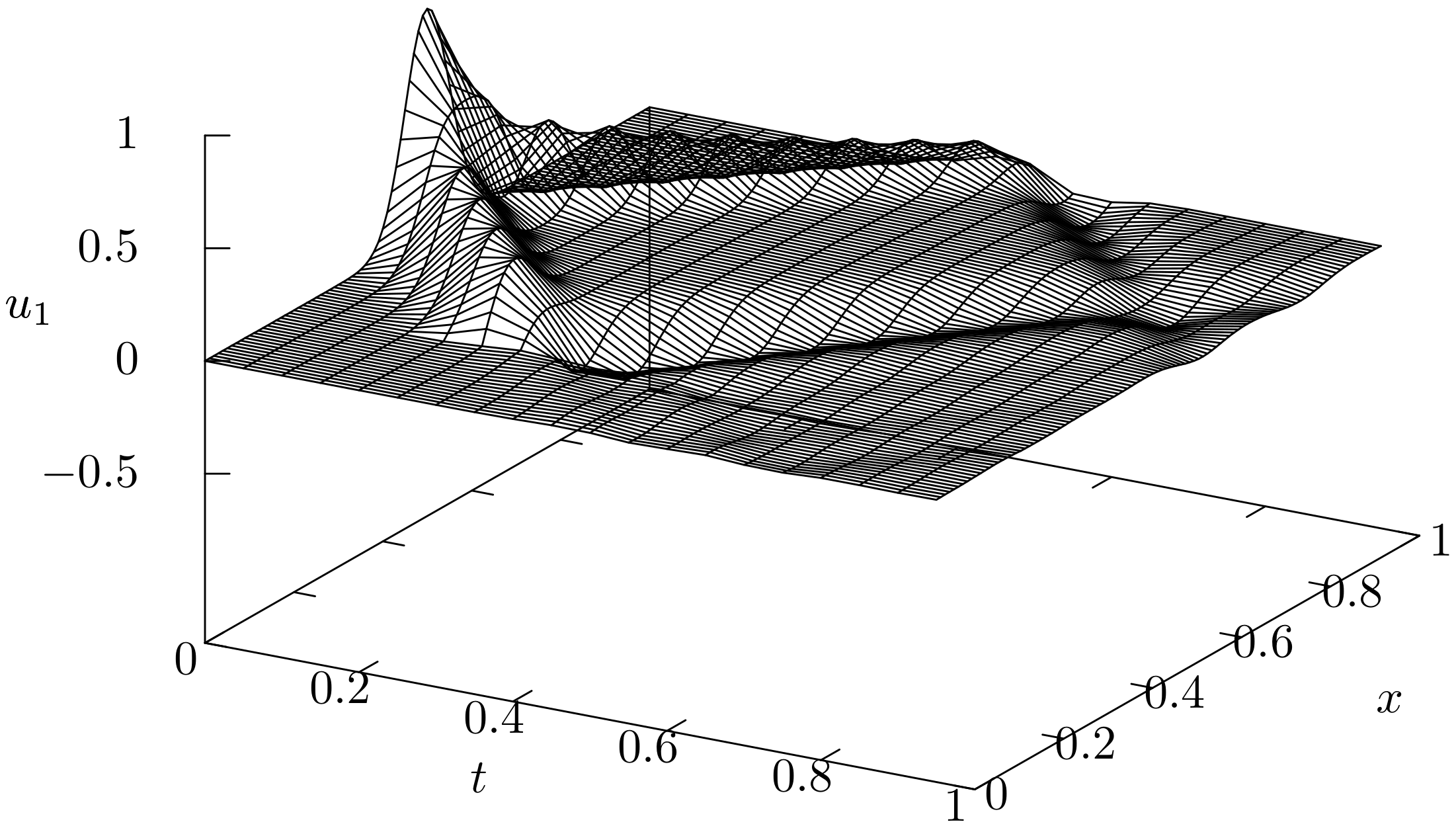
The positions of the interconnection are $x_1=x_2=0.2$. We first set the damping coefficients ${\gamma }_1$ and ${\gamma }_2$ to 0. The numerical solution from $t=0$ to $t=1.0$ are shown in Figure 2 and Figure 3. We observe that the wave packet shown in the initial state of the wave equation splits and propagates towards the connecting point and the right boundary. Then, at the connecting point, the wave packet is reflected while a slow wave is excited in the elastic equation.

Figure 2. The numerical solution of the wave in Equation (87) without the damping terms. The waves are partly reflected at the connecting point $x=x_1=0.2$.

Figure 3. The numerical solution of the elastic in Equation (88) without the damping terms. Although there exist no wave in the initial state, some waves are excited due to the energy exchange.

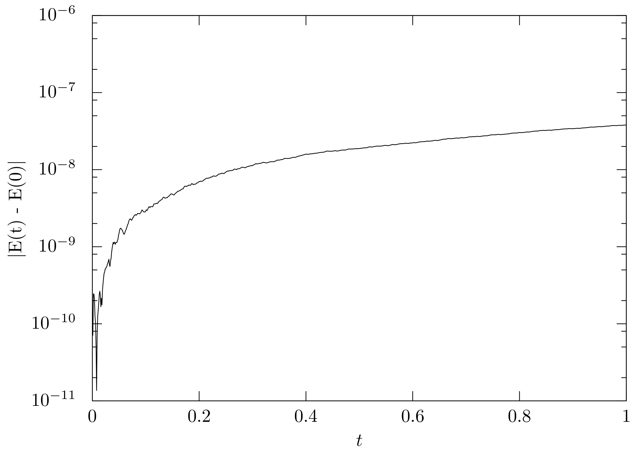
Although this causes an energy exchange, the total energy is preserved up to the rounding errors, as shown in Figure 4. In addition, in this example, if the energy is bounded, then $\parallel {\left(v_1\right)}^{\left(n\right)}{\parallel }_{L^2}$, $\parallel {\left(v_2\right)}^{\left(n\right)}{\parallel }_{L^2}$, $\parallel {\delta }_x^{+}{\left(u_1\right)}^{\left(n\right)}{\parallel }_{L^2}$, $\parallel {\delta }_x^{-}{\left(u_1\right)}^{\left(n\right)}{\parallel }_{L^2}$, $\parallel {\delta }_x^{+}{\left(u_2\right)}^{\left(n\right)}{\parallel }_{L^2}$, and $\parallel {\delta }_x^{-}{\left(u_2\right)}^{\left(n\right)}{\parallel }_{L^2}$ are all bounded. In fact, the stability of the numerical scheme follows from these conservation laws because combined with the Dirichlet boundary condition and the boundedness of $\parallel {\delta }_x^{+}{\left(u_1\right)}^{\left(n\right)}{\parallel }_{L^2}$ and $\parallel {\delta }_x^{+}{\left(u_2\right)}^{\left(n\right)}{\parallel }_{L^2}$ shows that $\parallel {\left(u_1\right)}^{\left(n\right)}{\parallel }_{L^{\infty }}$ and $\parallel {\left(u_2\right)}^{\left(n\right)}{\parallel }_{L^{\infty }}$ are also bounded from the discrete Poincaré inequality [13].

Figure 4. The deviation of the total energy in Equation (91) from the initial value of the coupled systems in Equations (87)–(89) without the damping terms. The energy is preserved up to the accumulation of the rounding errors.

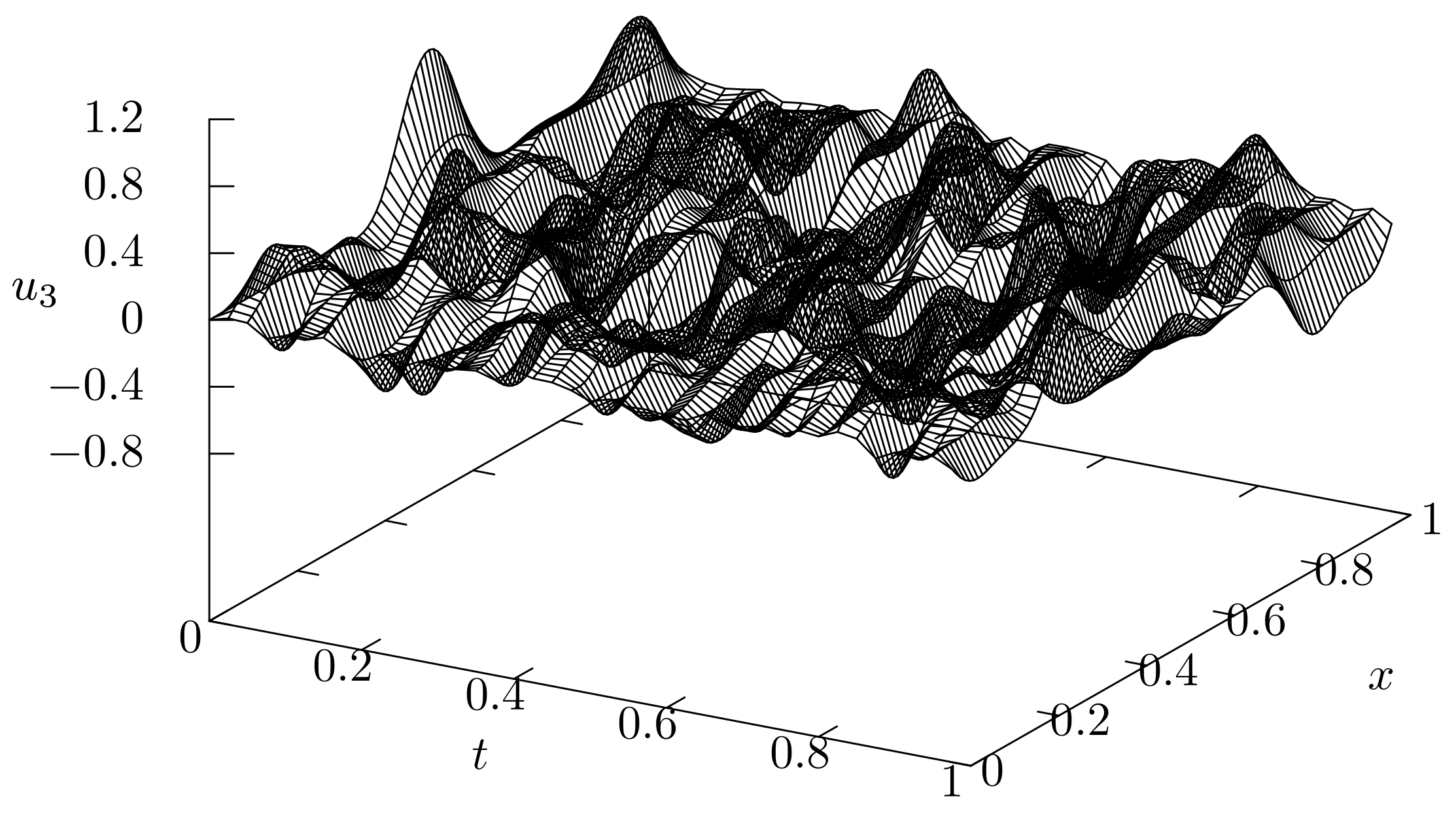
Second, we set both the damping coefficients ${\gamma }_1$ and ${\gamma }_2$ to 10. The numerical solution and the total energy from $t=0$ to $t=1.0$ are shown in Figure 5, Figure 6 and Figure 7, respectively. In particular, from the results in Figure 7, it is confirmed that the total energy is monotonically dissipated.

Figure 5. The numerical solution of the wave in Equation (87) with the damping terms. The waves are gradually dissipated.

Figure 6. The numerical solution of the elastic in Equation (88) with the damping terms. The excitation due to the energy exchange is smaller than that in the case without the damping terms.

Figure 7. The total energy inEquation (91) of the coupled systems in Equations (87)—(89) with the damping terms. The energy is rapidly dissipated.

The second example is a combination of the mass–spring system and the elastic equation:

$$\begin{array}{cc}\hfill & m_1\frac{{\mathrm{d}}^2{u}_1}{\mathrm{d}{t}^2}=-k(u_1-u_2)+f,m_2\frac{{\mathrm{d}}^2{u}_2}{\mathrm{d}{t}^2}=-k(u_2-u_1),\hfill \end{array}$$

(96)

$$\begin{array}{cc}\hfill & \rho \frac{{\partial }^2{u}_3}{\partial t^2}=-\frac{{\partial }^4{u}_3}{\partial x^4}-f\delta (x-x_0)(x\in (0,L)),\hfill \end{array}$$

(97)

$$\begin{array}{cc}\hfill & f=\frac{1}{\rho +m_1}\left(-m_1{\left.\frac{{\partial }^4{u}_3}{\partial x^4}\right|}_{x=x_0}+\rho k(u_1-u_2)\right).\hfill \end{array}$$

(98)

In this system, one side $u_1$ of the spring is attached to the elastic rod at $x=x_0$, while the other side $u_2$ is not constrained. The total energy is

$$\begin{array}{cc}\hfill E\left(t\right)=& \frac{m_1}{2}{\left(\frac{\mathrm{d}{u}_1}{\mathrm{d}t}\right)}^2+\frac{k}{2}{(u_1-u_2)}^2+\frac{m_2}{2}{\left(\frac{\mathrm{d}{u}_2}{\mathrm{d}t}\right)}^2+{\int }_0^L\left[\frac{\rho }{2}{\left(\frac{\partial u_3}{\partial t}\right)}^2+\frac{1}{2}{\left(\frac{{\partial }^2{u}_3}{\partial x^2}\right)}^2\right]\mathrm{d}x.\hfill \end{array}$$

(99)

The numerical scheme for this system is

$$\begin{array}{c}{\delta }_t^{+}{u}_1^{\left(n\right)}={\mathcal{A}}_t^{+}{v}_1^{\left(n\right)},m_1{\delta }_t^{+}{v}_1^{\left(n\right)}=-k{\mathcal{A}}_t^{+}\left(u_1^{\left(n\right)}-u_2^{\left(n\right)}\right)+f,\hfill \\ {\delta }_t^{+}{u}_2^{\left(n\right)}={\mathcal{A}}_t^{+}{v}_2^{\left(n\right)},m_2{\delta }_t^{+}{v}_2^{\left(n\right)}=-k{\mathcal{A}}_t^{+}\left(u_2^{\left(n\right)}-u_1^{\left(n\right)}\right),\hfill \\ {\delta }_t^{+}{\left(u_3\right)}_j^{\left(n\right)}={\mathcal{A}}_t^{+}{\left(v_3\right)}_j^{\left(n\right)},\rho {\delta }_t^{+}{\left(v_3\right)}_j^{\left(n\right)}=-{\delta }_x^{⟨4⟩}{\mathcal{A}}_t^{+}{\left(u_3\right)}_j^{\left(n\right)}-\frac{f}{\Delta x}{e}_l,\hfill \\ f=\frac{\Delta x}{\rho \Delta x+m_1}\left(-m_1{\mathcal{A}}_t^{+}{\delta }_x^{⟨4⟩}{\left(u_3\right)}_j^{\left(n\right)}+\rho k{\mathcal{A}}_t^{+}\left(u_1^{\left(n\right)}-u_2^{\left(n\right)}\right)\right),\hfill \end{array}$$

(100)

where l is the connecting point of the elastic equation and the term $f/\Delta x$ is an approximation to the delta function. The boundary condition for the elastic equation is the same as the previous example. The discrete total energy of this system is

$$\begin{array}{cc}\hfill E^{\left(n\right)}=& \frac{m_1}{2}{\left({\delta }_t^{+}{u}_1^{\left(n\right)}\right)}^2+\frac{k}{2}{(u_1^{\left(n\right)}-u_2^{\left(n\right)})}^2+\frac{m_2}{2}{\left({\delta }_t^{-}{u}_2^{\left(n\right)}\right)}^2\hfill \\ \hfill & +\sum _{j=1}^N\left[\frac{\rho }{2}{\left({\delta }_t^{+}{\left(u_3\right)}_j^{\left(n\right)}\right)}^2+\frac{1}{2}{\left({\delta }_x^{⟨2⟩}{\left(u_3\right)}_j^{\left(n\right)}\right)}^2\right]\Delta x.\hfill \end{array}$$

(101)

N denotes the number of the nodes. The initial conditions are given as

$$\begin{array}{c}{u}_1\left(0\right)=0,\frac{\mathrm{d}{u}_1}{\mathrm{d}t}\left(0\right)=0,u_2\left(0\right)=0,\frac{\mathrm{d}{u}_2}{\mathrm{d}t}\left(0\right)=0,u_3(0,x)=exp(-200{(x-\frac{1}{2})}^2),\frac{\partial u_3}{\partial t}(0,x)=0.\hfill \end{array}$$

(102)

The parameters are set to $m_1=m_2=\rho =1$, $k=1000$ and $\Delta t=0.001$. The elastic equation is solved on the interval $[0,1]$ and the connecting point is $x=0.8$. We set $N=100$.

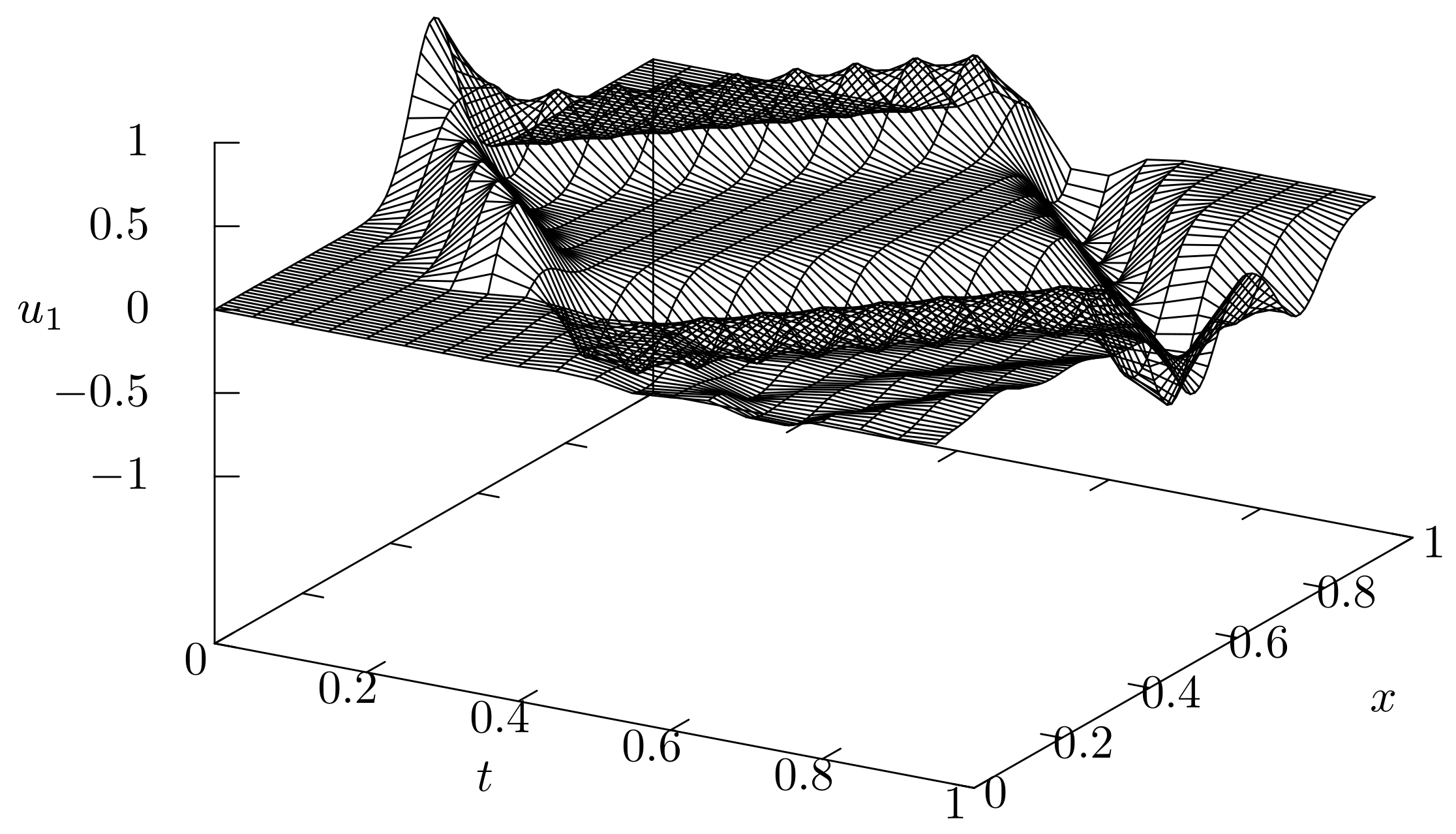
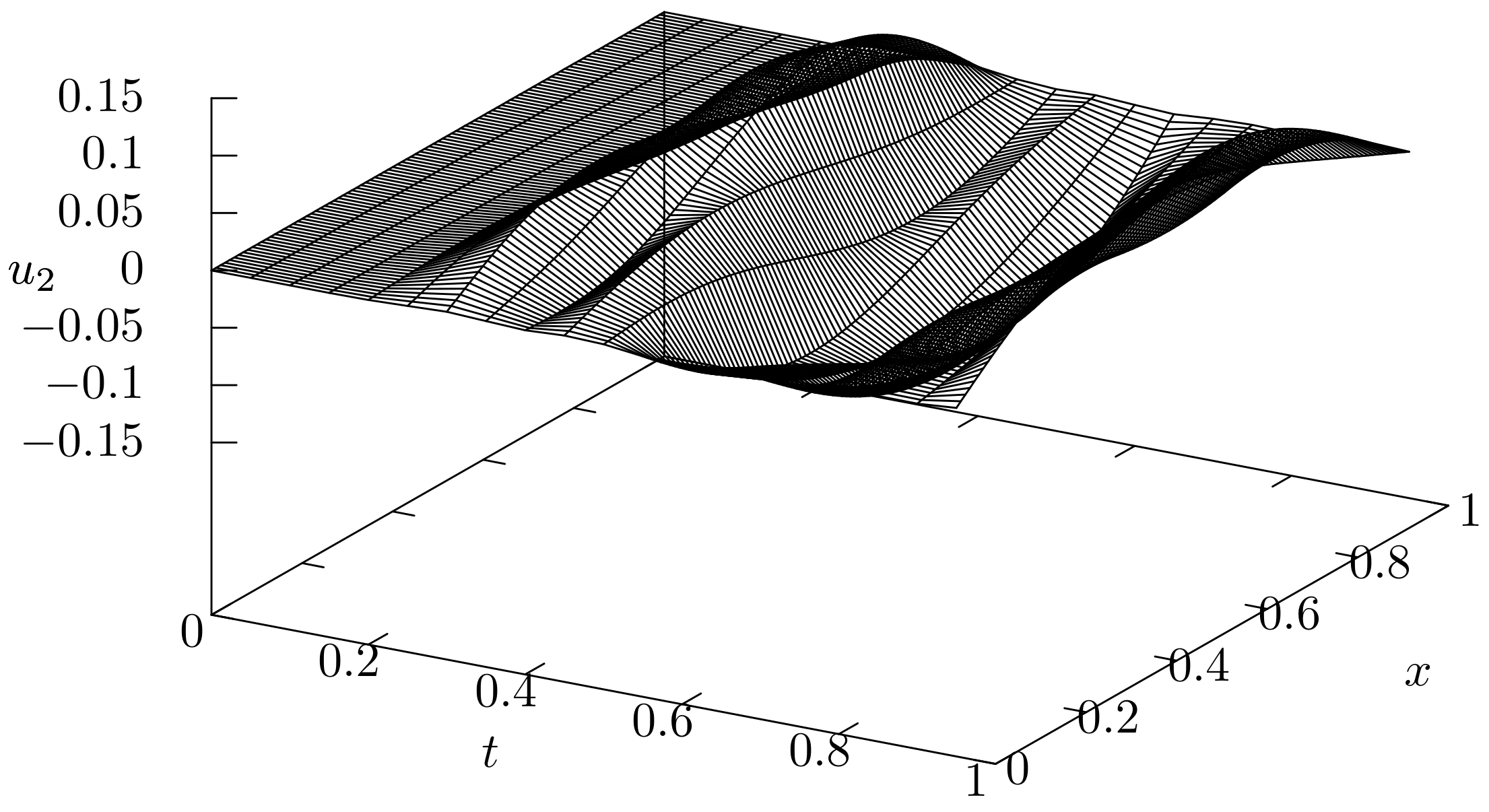
The numerical solutions for the mass–spring system $u_1$ and $u_2$ are shown in Figure 8 and that for the elastic equation $u_3$ in Figure 9. In this case, although the state variables of the mass–spring system is set to $u_1=u_2=0$ at $t=0$, they are excited by the energy exchange with the elastic bar through the connecting point. 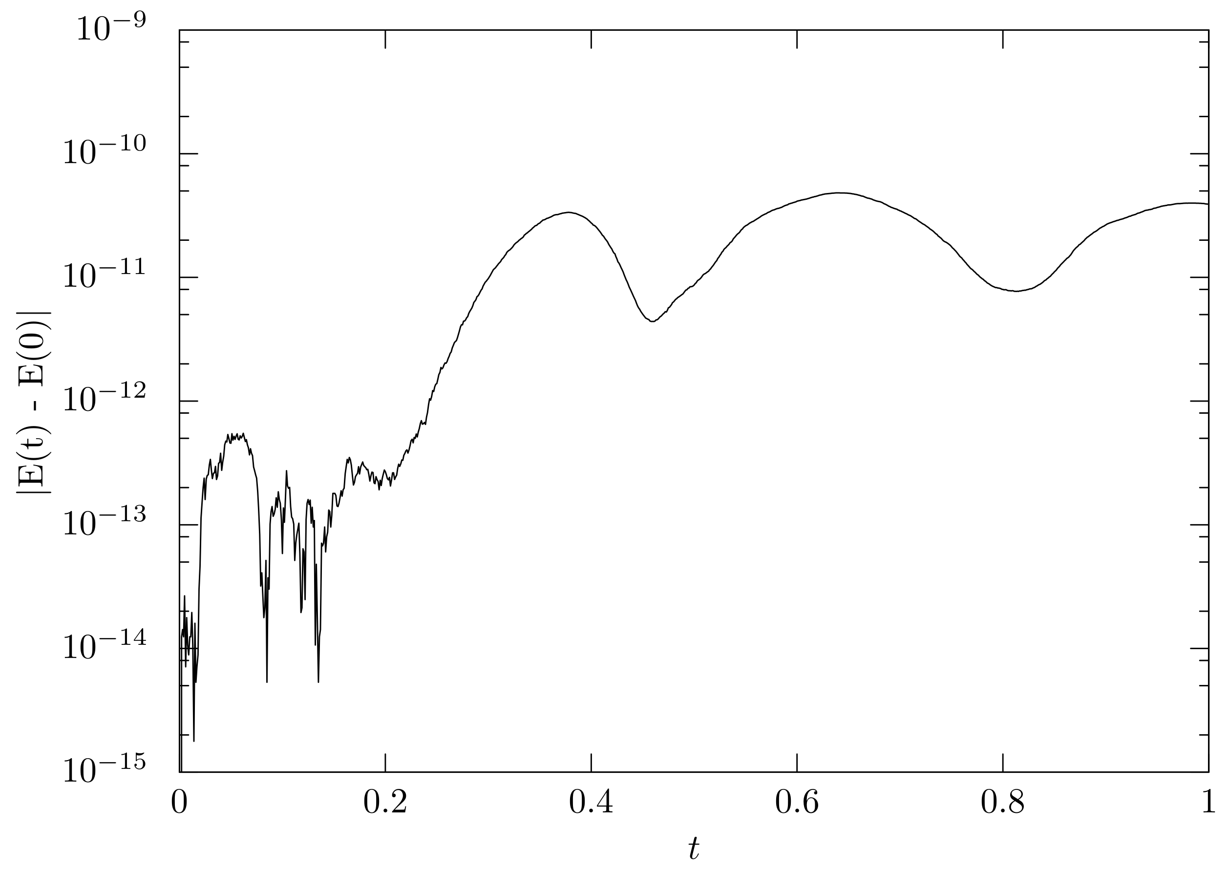The solution curve of $u_2$ is interestingly much smoother than that of $u_1$; this shows that the mass–spring system serves as a shock absorber. The deviation of the total energy from the initial state is shown in Figure 10. The total energy is preserved up to the accumulation of the rounding errors.

Figure 8. The computed behaviors of the both sides of the spring in Equation (96). The curve for the free side is much smoother than the other, which shows that this spring serves as a shock absorber.

Figure 9. The numerical solution to the elastic in Equation (97), which is connected at $x=0.8$ to a mass-spring system in Equation (96).

Figure 10. The deviation of the total energy in Equation (99) from the initial state. The energy is conserved up to the rounding errors.

6. Concluding Remarks

In this paper, we design energetic-property-preserving numerical methods for coupled natural systems. For such methods for coupled systems, Celledoni and Høiseth proposed energy-preserving numerical methods [8] aiming at controlling port-Hamiltonian systems. In this paper, we consider similar but slightly different models; restricting the target systems to natural systems, we coupled two systems by using the law of action–reaction. When the two systems with no dissipation term are coupled, it is essentially required that the time derivative of the state variables of the two systems are equal at the connecting point for conservation of the total energy. The model and the energetic-property-preserving numerical methods are constructed by determining the interaction between the systems so that this condition holds. As shown in the first numerical experiment, the conservation of energy often leads to the stability of numerical schemes. Such a systematic approach for deriving stable schemes is useful for simulations of large coupled systems because it is generally difficult to derive stable numerical methods for the complex systems.

For future work, the proposed technique should be applied for deriving stable numerical schemes for complicated systems that actually appear in industrial applications. In addition, because the proposed approach in this paper is based on the discrete gradient method, this approach derives implicit methods, which are not often feasible for large-scale systems. Therefore, it is important to develop a method for relaxing the derived implicit schemes to be explicit. For symplectic integrators, Tao proposed a method for rewriting any Hamiltonian system to a separable Hamilton system so that explicit numerical schemes are derived by using the splitting method [14]. It is desirable to develop explicit energetic-property-preserving numerical methods for coupled systems by using such a method.