Developing a New Robust Swarm-Based Algorithm for Robot Analysis

Abstract

Metaheuristics are incapable of analyzing robot problems without being enhanced, modified, or hybridized. Enhanced metaheuristics reported in other works of literature are problem-specific and often not suitable for analyzing other robot configurations. The parameters of standard particle swarm optimization (SPSO) were shown to be incapable of resolving robot optimization problems. A novel algorithm for robot kinematic analysis with enhanced parameters is hereby presented. The algorithm is capable of analyzing all the known robot configurations. This was achieved by studying the convergence behavior of PSO under various robot configurations, with a view of determining new PSO parameters for robot analysis and a suitable adaptive technique for parameter identification. Most of the parameters tested stagnated in the vicinity of strong local minimizers. A few parameters escaped stagnation but were incapable of finding the global minimum solution, this is undesirable because accuracy is an important criterion for robot analysis and control. The algorithm was trained to identify stagnating solutions. The algorithm proposed herein was found to compete favorably with other algorithms reported in the literature. There is a great potential of further expanding the findings herein for dynamic parameter identification.

1. Introduction

The quest for developing improved techniques for parameter identification of industrial robots has resulted in the novel concept of a mutating particle swarm optimization (MuPSO) based algorithm for analyzing multi-degree of freedom robot manipulators which was briefly introduced in [1], the research sought to employ artificial intelligence, particularly population-based Evolutionary Algorithms (EA), and computational methods for solving kinematic and dynamic problems of industrial manipulators. A robot manipulator is an electro-mechanical device that depicts the upper human limb. It was originally used in industrial workspaces to carry out tasks that were deemed boring, repetitive, highly monotonous, or dangerous, and therefore not suitable for human labor. Recent applications of robot manipulators include aeronautics and medicine, where the tolerance is very tight and human errors could be fatal. A robot manipulator comprises of solid non-moveable links connected by joints which allow either rotational or translational motion between successive links.

The increasing demand for robot manipulators has required that the manipulators become more autonomous and therefore increased accuracy and stability. The kinematic problems of robot manipulators were traditionally computed using analytical techniques which sometimes required finding the derivative of computationally expensive functions. These problems were found to sometimes possess multiple solutions or even no solution at all. Recently, swarm-based techniques have been studied which promises improved computational efficiency.

1.1. Swarm Intelligence

Evolutionary computation algorithms (EA) are stochastic optimization methods which have proven suitable for solving complex structured optimization and combinatory problems typical of robot analysis. They are biologically inspired population-based techniques that have relatively simple structures which are robust and computationally efficient. A variety of these algorithms have been developed over the years but based on simple implementation and the ability to readily combine with other algorithms, the PSO algorithm stands out. PSO was initially introduced by [2], despite being amongst the earliest EA algorithms, PSO remains relevant as it is still being improved, enhanced, and modified for solving real-world optimization problems.

In additive manufacturing (3D printing), constructing over-hanging features can only be achieved by introducing some support structures beneath the overhang which can be removed afterward to get the desired shape, [3] used a hybrid variation of PSO with greedy algorithm to reduce the volume of the support structure thereby save printing time, material and minimize budget. The recent hype in groundbreaking fifth-generation (5G) wireless communication technology presents the need to improve the quality of service with massive multiple-input multiple-output (MIMO) antenna arrays, [4] used a contraction adaptive PSO to optimize the design and positions of antenna array elements. Inspired by the success achieved by the proportional integral derivative (PID) controller in automation and its vast industrial applications [5,6,7] attempted using PID techniques to improve the performance of PSO. Reference [8] proposed the novel PID based strategy PSO (PBSPSO) algorithm based on the PID controller which was found to improve convergence while reducing stagnation of the PSO algorithm. A new variant of PSO with cross-over operation (PSOCO) was introduced by [9] which improved divergent search abilities of the PSO while avoiding stagnation by implementing a new learning model for the particles’ velocity formula and two cross-over operations, while [10] used PSO and multi-objective PSO to develop a two-stage auto-tuning technique for PID controllers. Automation of logistics, maintenance/support, storage, and others have led to rapid improvements in the vehicle routing problem (VRP) algorithm. The pick-up and delivery problem (PDP) is an extension of the VRP which collects goods from suppliers or pick-up points and conveys them to the delivery points, [11] introduced a novel pick-up and delivery problem with transfers (PDPT) algorithm using a hybrid PSO and local search algorithm to minimize distance and maximize profit. A PSO variant based on random perturbation (RP-PSO) was used to identify the parameters of a model pressurized water reactor nuclear power plant in [12]. The estimation of distribution algorithm (EDA) framework has been demonstrated in [13] to have high performance despite little memory requirements, it was combined with PSO in [14] and was used to estimate and preserve the distribution information of particles’ historical memories (personal best positions) to help the algorithm break out of local minimum solutions. The particle swarm estimation of distribution algorithms (PSDA) was also implemented in [15] for optimal-driven-projection of automated medical diagnosis and prognosis. Medical diagnosis is a key process in clinical medicine for identifying diseases, reducing cost, and enhancing accuracy. Enhanced algorithms were also exploited in [16,17,18] for diagnosis. Still, in medical sciences, minimally invasive surgery is a cost-effective alternative to open surgery where specialized instruments are used to operate by inserting them into several tiny punctures instead of one large incision. Reference [19] combined PSO with a back-propagation neural network (BPNN) algorithm to optimize the target position of the medical puncture robot.

1.2. Particle Swarm Optimization

The PSO consists of population members known as particles. Each particle refers to a bird in a flock, fish in a swarm, or in this case a possible solution to an optimization problem. The algorithm is initiated by populating it with n random particles, each particle has m dimensions, for the sake of robot analysis, the dimensions would be regarded as the degree of freedom (DOF). The position and velocity vectors of the ith particle can be defined as X_i and V_i in Equations (1) and (2) below. The position and velocity of every particle in the swarm is updated according to Equations (3) and (4) through every iteration, the first part of the Equation (3) is the previous velocity which describes the particles previous experience, the second part of the equation is the cognitive component which describes the particles personal experience while the third part of the equation is the social component which describes the entire swarms best experience. The inertia weight w is a learning coefficient associated with the previous velocity, while c₁ and c₂ are learning coefficients associated with the cognitive and social components respectively. The fitness function is a mathematical representation of the real-world problem to be analyzed, it evaluates how well the particles adapt to the actual solution of the problem. The leader of the swarm (fittest particle) is the particle that best adapts to the solution as it is updated through every iteration. The algorithm keeps a record of the solution of the fittest particle and also that of the best position achieved by each particle. The personal best position ever achieved by ith particle and global best position of the swarm is defined as P_iBest and G_iBest in Equations (5) and (6). The particles in the swarm would be seen to consistently move towards the solution of the problem through every iteration by updating the particle’s position, Equation (4), towards these two best memories (P_iBest and G_iBest).

$$X_i=\left(x_{i1},x_{i2},\dots ,x_{im}\right),$$

(1)

$${ \mathrm{V}}_i=\left(v_{i1},v_{i2},\dots ,v_{im}\right),$$

(2)

$$V_i(t+1)=w\cdot r\cdot V_i(t)+c_1\cdot r_1(P_{iBest}(t))-X_i(t)+c_2\cdot r_2(G_{iBest}(t)-X_i(t)),$$

(3)

$$X_i(t+1)=X_i(t)+V_i(t+1),$$

(4)

$$P_{iBest}=\left(p_{iBest},p_{iBest},\dots ,p_{iBest}\right),$$

(5)

$$G_{iBest}=\left(g_{iBest},g_{iBest},\dots ,g_{iBest}\right),$$

(6)

where r_j is a randomly generated number between [0, 1] and j ϵ [0, 1, 2]. PSO has a high convergence speed which is very desirable for robot applications, but this convergence speed sometimes results in stagnation which is a major limitation of the PSO algorithm. The characteristic of the PSO algorithm that allows it to define promising regions in search space is referred to as exploration while exploitation allows it to refine solutions within the defined promising region. These are the major characteristics of any PSO algorithm, a good algorithm balances these properties to find the best solution to a problem while avoiding stagnation. The contributions of [20] showed that these properties can be tuned by carefully selecting the value of w of the PSO algorithm. The concept of constriction coefficient was introduced, setting the inertia weight at 0.712 while the cognitive and social coefficient were both 1.494. This version of the PSO has come to be known today as the standard PSO (SPSO). The biological background of SPSO is believed to have evolved from the bird-like objects or BOIDS introduced by [21] to simulate flocking birds or animals in virtual reality studios. The BOIDS was governed by three basic rules; separation, alignment, and cohesion. The SPSO ignored the alignment and cohesion rules to reduce computational cost and increase convergence speed. Reference [22] proposed re-incorporating these rules reduces the convergence speed which is advantageous in pushing the algorithm out of stagnation. The effects of topologies on PSO were studied in [23], the SPSO has a star topology, where every individual is connected to other individuals such that information or direction of search is communicated and implemented throughout the swarm. Observing that this topology allows too much communication between the swarm particles and may be responsible for the quick convergence and stagnation of the SPSO, Reference [24] investigated the circle, wheel, and random topologies which isolate the individual particles of the swarm at different degrees so that information is communicated to the swarm by the focal individual or short-cuts between the isolated groups thereby causing a buffering effect which reduces the convergence speed of the swarm and improves search results. In [25], it was shown that the success of individual particles is not as a result of only the particle with the best fitness but by the influence of the entire swarm to a certain degree. An algorithm was presented that allowed every particle to have a weighted influence on other particles, based on their fitness such that particles with higher fitness exerted more influence. References [26,27] proposed the combination of SPSO with other computational search methods like conjugate gradient and steepest descent respectively. These variations of PSO also aimed at slowing down the convergence speed by allowing the algorithm to stop and search for promising regions in the local space, while [28] successfully merged PSO with ABC for nonlinear statistical analysis.

Swarms are best suited for analyzing static search spaces with one global solution (unimodal). In reality, most robot analysis problems contain more than one local solution (multimodal) and the search space is sometimes dynamic, therefore maintaining diversity is crucial for the performance of PSO. Various strains of PSO involving sub-swarms have been developed for this purpose, PSO was combined with expanding neighborhood topology in [29] to solve the permutation flow-shop scheduling problem. The algorithm is initiated with sub-swarms of small size neighborhoods, slowly expanding through every iteration, absorbing other particles, taking advantage of both the global and local neighborhood structures to increase the performance of the PSO algorithm. Competitive strategy was used in [30] to manage convergence, while entropy measurement was employed to maintain the diversity of the swarm. In [31], an adaptive multi-swarm competition PSO was proposed where the swarm is adaptively divided into sub-swarms and a competition mechanism is used to maintain diversity in the swarms. The sub-swarms slowly converge, adaptively reducing the number of swarms while balancing between exploration and exploitation tendencies. Other algorithms that employed sub-swarms include [32,33,34,35]. Although multi-swarm based algorithms were found to be efficient for solving multimodal problems, these algorithms have very high computational cost [33]. The new trends of adaptive SPSO where the inertia weight and acceleration components are altered during the search process is capable of improving exploration and exploitation tendencies with less computational cost [36]. In [37,38,39,40] the parameters of the adaptive PSO were dependent on the quality of the solution and tailored to the specific problem, the parameters were updated by comparing the values of the best particles (P_iBest and G_iBest). This technique was found favorable in analyzing both static and dynamic search spaces without incurring too much computational cost.

1.3. PSO and Robot Parameter Identification

Over the years, the use of PSO for robot parameter identification has been researched, a comparison between the linear least squares (LLS) method and the PSO was presented in [41] for the dynamic parameter identifications of a 3DOF Staubli RX-60 robot manipulator, where the PSO was found to produce better results. Reference [42] combined the linear simplification of the LLS and the non-linear optimization of the PSO for online and offline parameter identification of space robots. Space robots encounter changes in their kinematic parameters while running in the orbit. The non-linear model is first used for parameter identification in the offline mode while the LLS is used for online identification in the follow-up mission knowing that the parameters would not change much. These works and other similar research works exhibit the superiority of intelligent swarm-based techniques over traditional methods. A hybridized genetic algorithm and PSO (GAPSO) was implemented by [43] for parameter identification of a SCARA robot, [44] also implemented a hybridized BPNN and PSO for determining the kinematic parameters of a 6DOF robot manipulator, while [45] investigated the performance of seven PSO variants in solving the inverse kinematics of 2DOF robots. In [46,47], a combination of PSO and simulated annealing (SA) was used to optimize the geometric structure of non-redundant 6DOF manipulators. In [48] the Elitist Learning Strategy PSO (ELS-PSO) for dynamic parameter analysis of a 3DOF Staubli RX-60 robot manipulator. The Quantum-Behaved PSO (QPSO) was implemented for parameter identification of a puma 560 robot by [49] in two steps by first optimizing the individual joint parameters so that the identified values are close to the theoretical values, then all the joint parameters are further optimized simultaneously around the previously converged values. During the course of this research, it was observed that the solution for robot kinematic parameter identification problem did not converge under the basic parameters of the PSO especially when there were more than three degrees of freedom, and most published works implementing the PSO for robot parameter identification either used lower DOF robots or the algorithms were enhanced, modified and hybridized usually for specific robot manipulators, these algorithms are often not applicable for other robot configurations. Therefore, the concept of a novel Mutating PSO (MuPSO) algorithm was conceived for analyzing robot kinematics. To the best of our knowledge, there has not been any research tailored at determining the best range of PSO parameters to develop an algorithm for robot analysis, therefore this work aims to develop a new PSO variant capable of analyzing all robot configurations and least likely to fall into stagnation. This was achieved by first studying the behavior of PSO under various robot configurations and determining a new range of parameters for robot kinematic analysis, then a suitable adaptive technique was investigated and finally, the mutation function was implemented. A total of 54 different PSO parameters were tested on 6 robot manipulators. The rest of this paper is organized as follows; Section 2 presents the kinematic model of the robot configurations to be studied and the fitness function for the algorithm was formulated. Experiments studying the behavior of these robot configurations under various parameters were conducted in Section 3, the new adaptive strategy is presented in Section 4, comparing it with other variations of PSO. The results are presented in Section 5, the Mutation function was introduced in Section 6 and in Section 7 conclusions were drawn, while Section 8 presents the future thrust.

2. Kinematic Model of Robots

To determine a new set of parameters for robot analysis, the effect of four popular robot configurations was studied under various parameters. The robot configurations include the Articulate, Stanford, SCARA, and Dual-Arm robot configurations. These robot configurations were implemented on six different robot manipulators; the articulate configuration was implemented on a 3DOF robot manipulator because it is regarded as the most complex spatial robot configuration. The articulate robot configuration was also implemented on two different 6DOF robot manipulators of different sizes to study the effect of size on the PSO parameters.

2.1. Robot Configurations

Industrial manipulators usually have 6DOF as this gives the manipulator optimum dexterity, allowing it to complete most tasks in an industrial workspace. A robot with less than 6DOF is deficient, as it is easier to analyze and control but it cannot reach all the possible positions and orientations in its workspace. A redundant robot possesses more than 6DOF, they are more flexible, capable of maneuvering behind obstacles but more expensive to analyze and control. The SCARA manipulator is an example of a deficient robot manipulator, articulate manipulators are usually 6DOF while the dual-arm robot is a redundant manipulator (usually greater than 6DOF). It would be keen to note that the presence of a prismatic joint in any robot configuration simplifies the analysis while complicating the solution, it requires less computation but, like redundant configurations, there is a possibility of having numerous or even infinite solutions to every problem. The joints and end-effector of robots are always oriented along the z-axis of the coordinate frame.

• Scara Robot Configuration: The Selective Compliance Assembly Robot (SCARA) is one of the earliest industrial manipulators patented in 1981, it is usually a 4- or 5-DOF manipulator with all revolute joint, except one. In this analysis, a 4DOF SCARA manipulator shall be analyzed. The first joint of the manipulator being the prismatic joint, the other joints are revolute, parallel to each other and pointing along the direction of gravity. The SCARA manipulator is shown in Figure 1a and the DH-parameters are tabulated in

  Table 1. D-H Parameters for 4DOF SCARA arm.

  Joint	Link	Off-Set	Joint Displacement 1	Off-Set Displacement 2
  1	0	Variable (0–300)	0	0
  2	350	0	Variable (−pi/2–pi/2)	0
  3	350	0	Variable (−pi/2–pi/2)	0
  4	0	200	Variable (−pi/2–pi/2)	0

  For all DH parameters; ¹ joint displacement is Theta, ² off-set displacement of joint is Alfa, see Equations (7) and (8).

  .
• Articulate Robot Configuration: The articulate manipulator is the most popular robot configurations used in industrial workspaces, its analysis and solutions are trivial, therefore a very high accuracy can be achieved. All the joints of the articulated robot are revolute with the first joint pointing along the direction of gravity.
  The second third and fifth joints are parallel to each other and perpendicular to the first joint axis. The fourth and sixth joints are coincident and perpendicular to all the other joints. Three articulated manipulators were used in this analysis, one 3DOF articulated manipulator and two 6DOF articulated manipulators with significantly different sizes. The 3DOF articulate manipulator is configured exactly like the first three joints of the 6DOF articulate manipulator previously described. Figure 1b shows the 3DOF while Figure 2a shows the 6DOF robot configurations, their D-H parameters are tabulated in

  Table 2. D-H Parameters for 3DOF articulate arm.

  Joint	Link	Off-Set	Joint Displacement	Off-Set Displacement
  1	70	200	Variable (−pi/2–pi/2)	−pi/2
  2	150	0	Variable (−pi/2–pi/2)	0
  3	150	0	Variable (−pi/2–pi/2)	0

  ,

  Table 3. D-H Parameters for 6DOF articulate arm.

  Joint	Link	Off-Set	Joint Displacement	Off-Set Displacement
  1	64.5	170	Variable (−pi/2–pi/2)	−pi/2
  2	305	0	Variable (−pi/2–pi/2)	0
  3	0	0	Variable (−pi/2–pi/2)	pi/2
  4	0	−220	Variable (−pi/2–pi/2)	−pi/2
  5	0	0	Variable (−pi/2–pi/2)	pi/2
  6	0	−36	Variable (−pi/2–pi/2)	0

  and

  Table 4. D-H parameters for large 6DOF articulate arm

  Joint	Link	Off-Set	Joint Displacement	Off-Set Displacement
  1	300	320	Variable (−pi/2–pi/2)	−pi/2
  2	700	0	Variable (−pi/2–pi/2)	0
  3	0	0	Variable (−pi/2–pi/2)	−pi/2
  4	0	697.5	Variable (−pi/2–pi/2)	pi/2
  5	0	0	Variable (−pi/2–pi/2)	−pi/2
  6	0	127.5	Variable (−pi/2–pi/2)	0

  .
• Stanford Robot Configuration: The Stanford manipulator is also a 6DOF manipulator with five revolute joints and one prismatic joint. It is configured very much like the articulate arm except that the third arm is prismatic. The Stanford manipulator is shown in Figure 2b with its detailed D-H parameters defined in

  Table 5. D-H parameters for 6DOF Stanford arm.

  Joint	Link	Off-Set	Joint Displacement	Off-Set Displacement
  1	154	412	Variable (−pi/2–pi/2)	−pi/2
  2	0	0	Variable (−pi/2–pi/2)	0
  3	0	Variable (50–154)	−pi/2	−pi/2
  4	0	0	Variable (−pi/2–pi/2)	pi/2
  5	0	0	Variable (−pi/2–pi/2)	−pi/2
  6	0	263	Variable (−pi/2–pi/2)	0

  .
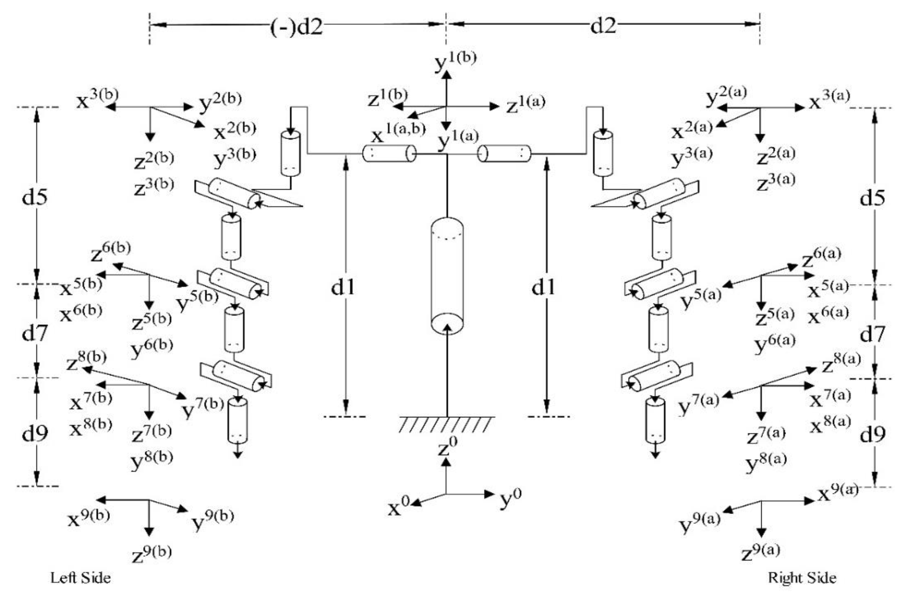
• Dual-Arm Robot Configuration: The dual-arm robot is the most dexterous of the manipulators with a total of 17DOF which are all revolute. It is configured such that the first joint at the ‘base’ of the structure is pointing along the direction of gravity. The third joint is parallel to the first joint and coincident with the fourth joint. The fifth, seventh, and ninth joints are also coincident with the third joint.

The fourth, sixth, and eight joints are parallel to each other and perpendicular to the first joint while the second joint is perpendicular to all the other joints. Figure 3 illustrates the dual-arm robot manipulator while

Table 6. D-H parameters for 17DOF dual-arm.

Joint	Link	Off-Set	Joint Displacement	Off-Set Displacement
1	0	400	th1	pi/2
2	0	200	Variable (−pi/2–pi/2) (a)	pi/2
		−200	Variable (−pi/2–pi/2) (b)	−pi/2
3	0	0	pi/2) (a)	0
		0	−pi/2) (b)	0
4	0	0	Variable (−pi/2–pi/2) (a)	−pi/2
		0	Variable (−pi/2–pi/2) (b)	pi/2
5	0	150	Variable (−pi/2–pi/2) (a)	pi/2
		−150	Variable (−pi/2–pi/2) (b)	−pi/2
6	0	0	Variable (−pi/2–pi/2) (a)	−pi/2
		0	Variable (−pi/2–pi/2) (b)	pi/2
7	0	150	Variable (−pi/2–pi/2) (a)	pi/2
		−150	Variable (−pi/2–pi/2) (b)	−pi/2
8	0	0	Variable (−pi/2–pi/2) (a)	−pi/2
		0	Variable (−pi/2–pi/2) (b)	pi/2
9	0	150	Variable (−pi/2–pi/2) (a)	0
		−150	Variable (−pi/2–pi/2) (b)	0

shows the D-H parameters of the robot.

2.2. Fitness Function

The homogeneous matrix of each successive pair of frames can be obtained using the formula in (7) below from the D-H parameters. the transformation matrix T for the robot manipulator’s end effector is a product of post multiplication as shown in the formula in (8).

$$T_{k-1}^k=\left[\begin{array}{cccc}\cos {\theta }_k& -\sin {\theta }_k& 0& a_k\\ \sin {\theta }_k\cos {\alpha }_{k-1}& \cos {\theta }_k\cos {\alpha }_{k-1}& -\sin {\alpha }_{k-1}& -d_k\sin {\alpha }_{k-1}\\ \sin {\theta }_k\sin {\alpha }_{k-1}& \cos {\theta }_k\sin {\alpha }_{k-1}& \cos {\alpha }_{k-1}& d_k\cos {\alpha }_{k-1}\\ 0& 0& 0& 1\end{array}\right],$$

(7)

$$T_0^{dof}=\left[\begin{array}{cccc}{t}_{11}& t_{12}& t_{13}& t_{14}\\ t_{21}& t_{22}& t_{23}& t_{24}\\ t_{31}& t_{32}& t_{33}& t_{34}\\ 0& 0& 0& 1\end{array}\right]=T_0^1{T}_1^2\cdots T_{dof-1}^{dof},$$

(8)

$$A=\left[\begin{array}{cccc}-0.5161& 0.2261& 0.8262& 349.5064\\ 0.7185& 0.6394& 0.2739& 1419.7\\ -0.4663& 0.7349& -0.4924& -516.5116\\ 0& 0& 0& 1\end{array}\right],$$

(9)

$$f_{ij}=t_{ij}-a_{ij},$$

(10)

$$Fitness={\displaystyle \sum _i^{n=3}{\displaystyle \sum _j^{m=4}(f_{ij}-E)}},$$

(11)

If the actual values of T read from sensors attached to the robot’s end-effector is given in A, then the fitness function (Fitness) would be as described in Equations (10) and (11). Where k ϵ [1, 2, …, dof], subscripts i, j ϵ [1, 2,…,4] and E = 1 × 10⁻⁸. Most robots are usually fitted with encoders, gyroscopes, and current controllers which can measure joint position, end-effector orientation, and actuator currents (torque) respectively. There are a variety of sensors that can also be mounted manually on robots.

3. Determining New PSO Parameters

An experiment aimed at studying the behavior of all popular robot configurations on different PSO parameters was performed to identify the best values of w and c that balances out exploration and exploitation tendencies while ensuring convergence of results and also to determine the solutions with the best computational efficiency. The initial value of w (w_i) was set to 0.7, increasing with an interval of 0.4 to a final value (w_f) at 1.5, such that w = 0.7:0.4:1.5. The initial value of c (c_i) was set at 1.5, increasing with an interval of 0.3 to a final value (c_f) at 3.9, such that c = 1.5:0.3:3.9 as elaborated in Figure 4. Then the experiment was repeated for c = 1.4:0.6:2.6 and w = 0.6:0.3:3.0. The 6 robot configurations were tested with 54 sets of PSO parameters in 30 generations and 2000 iterations. The mutation function was not implemented in this experiment, the results were tabulated and the performance of the PSO plotted. In

Table 7. Performance of PSO when w = 0.7.

Robot Configuration		PSO Parameters @ w = 0.7
		c = 1.5	c = 1.8	c = 2.1	c = 2.4	c = 2.7	c = 3.0	c = 3.3	c = 3.6	c = 3.9
3DOF Articulate Robot Arm	Average (Std)	1.1999 (0.996)	0.66662 (0.958)	0.99993 (1.017)	0.99993 (1.017)	0.8666 (1.008)	1.0666 (1.015)	0.99993 (1.017)	0.79994 (0.996)	0.8666 (1.008)
	Minimum	6.10 × 10−9	6.10 × 10−9	6.10 × 10−9	6.10 × 10−9	6.10 × 10−9	6.10 × 10−9	6.10 × 10−9	6.10 × 10−9	6.10 × 10−9
	Iteration	74.8	74.1	74.333	74.4	75.233	75.867	77.133	78.4	81.333
4DOF SCARA Robot Arm	Average (Std)	2.1333 (2.029)	1.7333 (2.016)	1.4667 (1.960)	2.1333 (2.029)	2.1333 (2.029)	2.2667 (2.016)	2.2667 (2.016)	1.7333 (2.02)	1.3333 (1.918)
	Minimum	9.73 × 10−10	9.73 × 10−10	9.73 × 10−10	9.73 × 10−10	9.73 × 10−10	9.73 × 10−10	9.73 × 10−10	9.73 × 10−10	9.73 × 10−10
	Iteration	78.967	78.067	78.467	79.233	79.5	81.233	82.733	85.433	87.267
6DOF Stanford Robot Arm	Average (Std)	2.4859 (2.145)	1.2563 (0.992)	1.2951 (1.049)	0.85651 (1.123)	0.28667 (0.751)	0.18892 (0.590)	0.10886 (0.509)	0.08696 (0.388)	0.015589 (0.0401)
	Minimum	4.67 × 10−4	3.21 × 10−2	1.05 × 10−4	4.31 × 10−7	1.68 × 10−6	1.32 × 10−6	5.80 × 10−9	5.80 × 10−9	5.80 × 10−9
	Iteration	533.4	508.3	554.1	511.8	417.4	601.4	567.6	651.57	643.47
6DOF Articulate Robot Arm (small)	Average (Std)	3.7837 (1.759)	1.5927 (1.237)	1.1403 (0.633)	0.80981 (0.506)	0.59953 (0.780)	0.24822 (0.412)	0.27092 (0.457)	0.17026 (0.385)	0.31949 (0.596)
	Minimum	1.11 × 100	3.48 × 10−1	9.21 × 10−2	8.27 × 10−2	2.83 × 10−9	2.83 × 10−9	2.83 × 10−9	2.83 × 10−9	2.83 × 10−9
	Iteration	261.87	235.43	265.87	260.93	296.7	214.53	166.63	170.67	157.63
6DOF Articulate Robot Arm (big)	Average (Std)	3.4266 (1.732)	2.9774 (1.649)	1.5511 (0.902)	1.3035 (1.180)	0.86441 (1.095)	0.43759 (0.784)	0.30934 (0.458)	0.35057 (0.680)	0.35187 (0.456)
	Minimum	6.53 × 10−1	7.02 × 10−1	5.70 × 10−2	7.09 × 10−2	6.98 × 10−4	5.53 × 10−9	5.53 × 10−9	5.53 × 10−9	5.53 × 10−9
	Iteration	244.33	230.5	285.63	343.43	416.5	375.47	327.27	323.77	377.8
17DOF Dual-Arm Robot Arm	Average (Std)	2.873 (2.307)	1.7774 (1.672)	0.71947 (0.803)	0.51867 (0.569)	0.25626 (0.425)	0.13317 (0.388)	0.14343 (0.469)	0.14844 (0.678)	0.13608 (0.419)
	Minimum	2.35 × 10−2	1.81 × 10−2	3.90 × 10−3	1.99 × 10−4	4.43 × 10−5	3.82 × 10−9	3.82 × 10−9	3.82 × 10−9	3.82 × 10−9
	Iteration	326.07	378.17	364.87	390.77	451.3	437.33	447.07	457.43	468.83

, the average and standard deviation of the best solutions after thirty runs and the solution that best minimizes the problem were presented, the average number of iterations required to find the best solution for each of the six robot manipulators was also presented at w = 0.7.

Table 8. Performance of PSO when w = 1.1

Robot Configuration		PSO Parameters @ w = 1.1
		c = 1.5	c = 1.8	c = 2.1	c = 2.4	c = 2.7	c = 3.0	c = 3.3	c = 3.6	c = 3.9
3DOF Articulate Robot Arm	Average (Std)	1.0666 (1.015)	1.1999 (0.996)	0.79994 (0.996)	0.99993 (1.017)	0.66662 (0.959)	1.3332 (0.959)	1.2666 (0.980)	1.1333 (1.008)	1.0666 (1.015)
	Minimum	6.10 × 10−9	6.10 × 10−9	6.10 × 10−9	6.10 × 10−9	6.10 × 10−9	6.10 × 10−9	6.10 × 10−9	6.10 × 10−9	6.10 × 10−9
	Iteration	81.6	81.7	81.267	82.267	83.9	85.733	87.667	91.1	96.533
4DOF SCARA Robot Arm	Average (Std)	2 (2.034)	2.2667 (2.016)	1.7333 (2.016)	2.1333 (2.03)	2.2667 (2.016)	1.8667 (2.03)	2.2667 (2.016)	2 (2.034)	2.2667 (2.016)
	Minimum	9.73 × 10−10	9.73 × 10−10	9.73 × 10−10	9.73 × 10−10	9.73 × 10−10	9.73 × 10−10	9.73 × 10−10	9.73 × 10−10	9.73 × 10−10
	Iteration	88.667	87.7	88.633	90.133	91.6	93.367	97.767	101.97	106
6DOF Stanford Robot Arm	Average (Std)	0.75869 (1.099)	0.71229 (1.079)	0.37784 (1.009)	0.27387 (0.758)	0.28313 (0.852)	0.02518 (0.059)	0.53394 (1.008)	0.19628 (0.561)	0.17413 (0.519)
	Minimum	7.02 × 10−5	1.06 × 10−5	4.14 × 10−6	5.80 × 10−9	5.80 × 10−9	5.80 × 10−9	5.80 × 10−9	5.80 × 10−9	5.80 × 10−9
	Iteration	661.17	637.47	581.6	590.93	548.53	648.57	585.13	648.67	810.17
6DOF Articulate Robot Arm (small)	Average (Std)	1.3059 (1.047)	0.71658 (0.695)	0.27506 (0.580)	0.46958 (0.945)	0.22999 (0.387)	0.32675 (0.611)	0.30032 (0.452)	0.46418 (0.779)	0.22069 (0.412)
	Minimum	9.23 × 10−3	3.23 × 10−3	2.83 × 10−9	2.83 × 10−9	2.83 × 10−9	2.83 × 10−9	2.83 × 10−9	2.83 × 10−9	2.83 × 10−9
	Iteration	375.67	385.77	367.23	193.1	186.47	162.57	178.2	190.97	246.33
6DOF Articulate Robot Arm (big)	Average (Std)	1.5539 (1.113)	0.82201 (0.625)	0.46599 (0.473)	0.30729 (0.433)	0.52439 (1.167)	0.49672 (0.635)	0.33982 (0.588)	0.48452 (0.488)	0.70028 (1.07)
	Minimum	6.30 × 10−2	2.71 × 10−2	3.28 × 10−7	5.53 × 10−9	5.53 × 10−9	5.53 × 10−9	5.53 × 10−9	5.53 × 10−9	5.53 × 10−9
	Iteration	341.5	532.1	553.77	405.8	311.9	293.23	352.83	315.17	483.03
17DOF Dual-Arm Robot Arm	Average (Std)	0.4248 (0.48)	0.09798 (0.131)	0.14656 (0.316)	0.11974 (0.248)	875.8 (4796.4)	0.068428 (0.151)	723.89 (3964.6)	0.18718 (0.324)	0.12041 (0.269)
	Minimum	5.31 × 10−3	3.60 × 10−4	5.10 × 10−5	3.82 × 10−9	3.82 × 10−9	3.82 × 10−9	3.82 × 10−9	3.82 × 10−9	3.82 × 10−9
	Iteration	501.6	562.43	483.93	444.2	432	422.9	422.1	440	611.93

and

Table 9. Performance of PSO when w = 1.5.

Robot Configuration		PSO Parameters @ w = 1.5
		c = 1.5	c = 1.8	c = 2.1	c = 2.4	c = 2.7	c = 3.0	c = 3.3	c = 3.6	c = 3.9
3DOF Articulate Robot Arm	Average (Std)	0.8666 (1.008)	0.9999 (1.017)	0.9333 (1.015)	1.0666 (1.015)	0.7999 (0.996)	1.3999 (0.932)	1.0666 (1.015)	0.7333 (0.980)	1.1999 (0.996)
	Minimum	6.10 × 10−9	6.10 × 10−9	6.10 × 10−9	6.10 × 10−9	6.10 × 10−9	6.10 × 10−9	6.10 × 10−9	6.10 × 10−9	6.10 × 10−9
	Iteration	93.633	94.333	95.1	97.6	101.53	104.93	111.3	119.9	130.03
4DOF SCARA Robot Arm	Average (Std)	2.4 (1.993)	1.8667 (2.03)	2.1333 (2.03)	2 (2.034)	2.2667 (2.016)	2.5333 (1.960)	1.6 (1.993)	1.7333 (2.016)	2 (2.034)
	Minimum	9.73 × 10−10	9.73 × 10−10	9.73 × 10−10	9.73 × 10−10	9.73 × 10−10	9.73 × 10−10	9.73 × 10−10	9.73 × 10−10	9.73 × 10−10
	Iteration	103.9	103.9	105.03	110.07	113.53	117	126.2	139.67	156.7
6DOF Stanford Robot Arm	Average (Std)	0.0169 (0.048)	0.1762 (0.58)	0.0927 (0.387)	0.0793 (0.382)	0.2655 (0.69)	0.1456 (0.462)	0.1750 (0.603)	0.2623 (0.748)	0.0996 (0.241)
	Minimum	5.80 × 10−9	5.80 × 10−9	5.80 × 10−9	5.80 × 10−9	5.80 × 10−9	5.80 × 10−9	5.86 × 10−9	6.77 × 10−9	6.72 × 10−7
	Iteration	784.03	764.1	728.07	689.4	664.9	839.4	1143.2	1273.1	1667.7
6DOF Articulate Robot Arm (small)	Average (Std)	0.4613 (0.735)	0.2363 (0.411)	0.3917 (0.629)	0.27185 (0.456)	0.7003 (0.841)	0.29195 (0.6)	0.38275 (0.474)	0.24172 (0.434)	0.42294 (0.499)
	Minimum	2.83 × 10−9	2.83 × 10−9	2.83 × 10−9	2.83 × 10−9	2.83 × 10−9	2.83 × 10−9	2.83 × 10−9	2.83 × 10−9	2.90 × 10−9
	Iteration	235.23	236.67	208.27	213.37	208.53	251.27	331.77	377.17	558.5
6DOF Articulate Robot Arm (big)	Average (Std)	0.3755 (0.616)	0.3122 (0.429)	0.2982 (0.602)	0.54127 (0.736)	0.24539 (0.422)	0.33632 (0.472)	0.33908 (0.666)	0.54117 (0.492)	0.60112 (0.79)
	Minimum	5.53 × 10−9	5.53 × 10−9	5.53 × 10−9	5.53 × 10−9	5.53 × 10−9	5.53 × 10−9	5.53 × 10−9	5.56 × 10−9	6.22 × 10−9
	Iteration	490.57	434.43	405.5	375.57	438.6	509.8	695.57	935.57	1374.1
17DOF Dual-Arm Robot Arm	Average (Std)	0.03969 (0.091)	0.1555 (0.349)	0.58298 (1.275)	0.12749 (0.280)	0.24011 (0.726)	0.25313 (0.850)	0.089832 (0.219)	0.31591 (0.629)	0.27926 (0.494)
	Minimum	3.82 × 10−9	3.82 × 10−9	3.82 × 10−9	3.82 × 10−9	3.82 × 10−9	3.82 × 10−9	3.82 × 10−9	3.84 × 10−9	4.09 × 10−9
	Iteration	566.6	419.9	412.63	538.6	571.17	587.53	911.87	945.53	1338

present a similar set of results for w at 1.1 and 1.5, respectively. To ease comparison and visualization of the results, a summary is presented in

Table 10. Aggregate of performance for PSO for different values of inertia weight (w).

Robot Configuration		PSO Parameters
		c = 1.5	c = 1.8	c = 2.1	c = 2.4	c = 2.7	c = 3.0	c = 3.3	c = 3.6	c = 3.9
3DOF Articulate Robot Arm	w = 0.7	0.02513	0.14763	0.06318	0.06297	0.09043	0.04511	0.05457	0.09739	0.07168
	w = 1.1	0.08921	0.06846	0.14458	0.09944	0.17200	0.04226	0.04449	0.05379	0.05053
	w = 1.5	0.16746	0.14006	0.15103	0.12242	0.16699	0.06913	0.09608	0.14758	0.04076
4DOF SCARA Robot Arm	w = 0.7	0.03849	0.08687	0.12197	0.03773	0.03696	0.01897	0.01468	0.06577	0.11672
	w = 1.1	0.07029	0.04539	0.10203	0.05269	0.03619	0.07446	0.02166	0.0389	0.00224
	w = 1.5	0.10249	0.15062	0.12251	0.12707	0.09746	0.07244	0.14586	0.10839	0.05263
6DOF Stanford Robot Arm	w = 0.7	0.29170	0.31301	0.53404	0.58656	0.72349	0.68145	0.71189	0.69607	0.74687
	w = 1.1	0.04599	0.28527	0.45162	0.55492	0.54350	0.77809	0.41407	0.60752	0.57449
	w = 1.5	0.84829	0.52364	0.67211	0.69225	0.41774	0.58066	0.46007	0.30967	0.32558
6DOF Articulate Robot Arm (small)	w = 0.7	0.02935	0.44219	0.58987	0.63601	0.59946	0.74424	0.77674	0.79026	0.76129
	w = 1.1	0.00654	0.35941	0.57088	0.55936	0.74264	0.68628	0.71899	0.60129	0.69970
	w = 1.5	0.26829	0.44414	0.33662	0.42852	0.16347	0.36172	0.33072	0.37207	0.20066
6DOF Articulate Robot Arm (big)	w = 0.7	0.12076	0.15641	0.56486	0.50314	0.52856	0.62945	0.71490	0.68191	0.68178
	w = 1.1	0.10744	0.38614	0.57372	0.67457	0.52483	0.65161	0.65997	0.67519	0.44003
	w = 1.5	0.33744	0.43315	0.38945	0.25154	0.46242	0.39587	0.29945	0.22558	0
17DOF Dual-Arm Robot Arm	w = 0.7	0.07612	0.26993	0.61418	0.68276	0.69043	0.71311	0.69829	0.66969	0.69280
	w = 1.1	0.54493	0.75326	0.79984	0.81848	0.32351	0.82719	0.41427	0.82017	0.74995
	w = 1.5	0.62593	0.55313	0.18953	0.55625	0.41449	0.38161	0.51477	0.33042	0.28333

showing the averages of normalized values obtained in Table 7, Table 8 and Table 9 while Figure 5a–f shows a pictorial plot of the performance of PSO for each of the robot manipulators. Similarly,

Table 11. Performance of PSO when c = 1.4.

Robot Configuration		PSO Parameters @ c = 1.4
		w = 0.6	w = 0.9	w = 1.2	w = 1.5	w = 1.8	w = 2.1	w = 2.4	w = 2.7	w = 3.0
3DOF Articulate Robot Arm	Average (Std)	0.73328 (0.980)	0.79994 (0.996)	0.66662 (0.959)	1.2666 (0.980)	0.73328 (0.980)	0.93327 (1.015)	0.99994 (1.017)	0.73819 (0.978)	1.0239 (1.018)
	Minimum	6.10 × 10−9	6.10 × 10−9	6.10 × 10−9	6.10 × 10−9	6.10 × 10−9	6.10 × 10−9	1.31 × 10−8	3.26 × 10−5	7.19 × 10−4
	Iteration	74.3	78.033	83.933	93.667	111.1	163.37	232.83	194.1	148.43
4DOF SCARA Robot Arm	Average (Std)	1.8667 (2.03)	1.7333 (2.016)	2.2667 (2.016)	2.2667 (2.016)	2 (2.034)	1.7333 (2.016)	2.1337 (2.03)	2.0962 (2.004)	3.1436 (2.001)
	Minimum	9.73 × 10−10	9.73 × 10−10	9.73 × 10−10	9.73 × 10−10	9.73 × 10−10	9.75 × 10−10	1.55 × 10−6	1.79 × 10−3	1.40 × 10−2
	Iteration	79.5	83.367	91	105.17	130.5	206.57	308.47	187.27	157.93
6DOF Stanford Robot Arm	Average (Std)	2.5438 (1.583)	1.2003 (0.786)	0.52798 (0.625)	0.097716 (0.141)	0.35949 (0.813)	0.32893 (0.483)	0.77691 (0.806)	1.7795 (1.523)	2.3766 (1.732)
	Minimum	1.51 × 10−1	9.36 × 10−2	3.03 × 10−4	5.80 × 10−9	5.91 × 10−9	3.63 × 10−7	4.73 × 10−2	3.86 × 10−3	5.43 × 10−2
	Iteration	262.63	306.27	642.43	435.93	499.73	1470.9	1207.9	310.93	248.13
6DOF Articulate Robot Arm (small)	Average (Std)	4.6704 (1.794)	2.1154 (1.661)	0.82515 (0.557)	0.22069 (0.412)	0.4114 (1.166)	0.51296 (0.829)	1.2454 (1.115)	4.4305 (2.404)	4.6366 (1.966)
	Minimum	1.21 × 10−1	3.65 × 10−1	1.47 × 10−3	2.83 × 10−9	2.83 × 10−9	2.99 × 10−9	2.33 × 10−2	4.50 × 10−1	1.44 × 100
	Iteration	235.63	275.37	484.83	287.63	285.87	966.1	958.5	195.5	149.53
6DOF Articulate Robot Arm (big)	Average (Std)	4.1872 (1.933)	3.1769 (1.566)	1.2053 (0.941)	0.33989 (0.610)	0.44367 (0.68)	0.68313 (1.127)	4.4449 (2.091)	4.6878 (2.046)	5.856 (2.395)
	Minimum	1.64 × 10−1	2.00 × 10−1	2.27 × 10−2	5.53 × 10−9	5.53 × 10−9	8.06 × 10−8	2.35 × 10−1	1.87 × 100	1.89 × 100
	Iteration	215.27	302.93	744.57	518.87	555.8	1648.6	316.07	177.73	153.57
17DOF Dual-Arm Robot Arm	Average (Std)	3.498 (2.36)	1.446 (1.482)	0.57004 (1.077)	0.32323 (1.048)	0.1926 (0.663)	0.31277 (0.748)	1.253 (1.894)	3.564 (2.658)	3.7033 (2.702)
	Minimum	3.11 × 10−1	9.79 × 10−2	1.88 × 10−4	3.82 × 10−9	3.82 × 10−9	3.76 × 10−8	4.11 × 10−3	1.56 × 10−1	6.29 × 10−2
	Iteration	372.1	390.1	749.33	641.27	717.17	1487.3	840.23	222.47	167.8

,

Table 12. Performance of PSO when c = 2.0.

Robot Configuration		PSO Parameters @ c = 2.0
		w = 0.6	w = 0.9	w = 1.2	w = 1.5	w = 1.8	w = 2.1	w = 2.4	w = 2.7	w = 3.0
3DOF Articulate Robot Arm	Average (Std)	1.2666 (0.980)	1.0666 (1.015)	0.79994 (0.996)	1.1333 (1.008)	1.2666 (0.980)	1.1333 (1.008)	1.0668 (1.015)	0.87109 (1.009)	1.2906 (0.996)
	Minimum	6.10 × 10−9	6.10 × 10−9	6.10 × 10−9	6.10 × 10−9	6.10 × 10−9	6.14 × 10−9	4.64 × 10−6	3.20 × 10−4	2.23 × 10−4
	Iteration	72.2	77.133	83.2	94.767	116.83	188.97	234.67	177.8	160.8
4DOF SCARA Robot Arm	Average (Std)	2.5333 (1.960)	1.6 (1.993)	1.4667 (1.960)	1.4667 (1.960)	1.3333 (1.918)	2.1333 (2.03)	1.7349 (2.017)	2.3599 (2.030)	2.766 (2.038)
	Minimum	9.73 × 10−10	9.73 × 10−10	9.73 × 10−10	9.73 × 10−10	9.73 × 10−10	1.09 × 10−9	3.84 × 10−7	3.16 × 10−3	2.99 × 10−2
	Iteration	76.533	82.733	91.7	105.2	135.63	241.73	241.67	168.1	172
6DOF Stanford Robot Arm	Average (Std)	1.3284 (1.109)	0.81005 (0.726)	0.21514 (0.525)	0.14129 (0.178)	0.18694 (0.239)	0.35786 (0.465)	1.0369 (0.939)	3.3027 (8.697)	2.3353 (1.637)
	Minimum	1.11 × 10−4	2.88 × 10−4	6.62 × 10−7	5.80 × 10−9	2.84 × 10−8	4.72 × 10−7	5.75 × 10−2	3.22 × 10−1	2.23 × 10−1
	Iteration	262.17	343.6	482.7	407.93	686.8	1528.3	922.13	433.7	230.27
6DOF Articulate Robot Arm (small)	Average (Std)	1.8589 (1.261)	0.77962 (0.727)	0.47691 (0.630)	0.29102 (0.703)	0.42741 (0.633)	0.37187 (0.476)	2.0606 (1.968)	4.4253 (1.984)	4.2691 (1.984)
	Minimum	3.62 × 10−1	4.90 × 10−2	2.83 × 10−9	2.83 × 10−9	2.83 × 10−9	4.88 × 10−9	3.23 × 10−2	2.99 × 10−1	6.28 × 10−1
	Iteration	274.63	288.7	248.77	224.4	302.47	1291.5	698.8	222.47	170.67
6DOF Articulate Robot Arm (big)	Average (Std)	2.791 (1.543)	1.018 (0.532)	0.41474 (0.622)	0.34059 (0.61)	0.36141 (0.621)	1.1712 (1.458)	3.9099 (2.242)	4.9021 (2.015)	5.8541 (2.339)
	Minimum	7.32 × 10−1	1.39 × 10−2	5.53 × 10−9	5.53 × 10−9	5.53 × 10−9	3.10 × 10−2	5.18 × 10−1	1.41 × 100	1.28 × 100
	Iteration	217.1	339.4	518.1	430.33	600.13	1428.2	293.03	185	157.67
17DOF Dual-Arm Robot Arm	Average (Std)	725.92 (3965.7)	0.56706 (0.482)	0.12174 (0.205)	0.10393 (0.219)	0.1511 (0.329)	0.28911 (0.646)	0.84244 (1.004)	3.791 (2.441)	3.6224 (2.501)
	Minimum	1.03 × 10−1	2.38 × 10−3	3.82 × 10−9	3.82 × 10−9	3.82 × 10−9	2.09 × 10−4	7.55 × 10−3	5.07 × 10−1	9.86 × 10−2
	Iteration	343.93	426.93	486.23	500.5	787.8	1574.7	676.1	205.9	172.47

,

Table 13. Performance of PSO when c = 2.6.

Robot Configuration		PSO Parameters @ c = 2.6
		w = 0.6	w = 0.9	w = 1.2	w = 1.5	w = 1.8	w = 2.1	w = 2.4	w = 2.7	w = 3.0
3DOF Articulate Robot Arm	Average (Std)	1.1333 (1.008)	0.66662 (0.959)	0.93327 (1.015)	0.93327 (1.015)	0.8666 (1.008)	0.9333 (1.015)	1.0005 (1.017)	0.9414 (1.012)	0.74984 (0.980)
	Minimum	6.10 × 10−9	6.10 × 10−9	6.10 × 10−9	6.10 × 10−9	6.10 × 10−9	6.48 × 10−9	8.80 × 10−7	1.47 × 10−3	7.17 × 10−7
	Iteration	72.833	79.533	86.8	99.633	132.5	240.2	178.6	139.67	126.83
4DOF SCARA Robot Arm	Average (Std)	2.6667 (1.918)	1.4667 (1.960)	2.2667 (2.016)	2.2667 (2.016)	2.4 (1.993)	1.8667 (2.03)	1.8716 (2.03)	2.3128 (2.103)	2.5558 (1.99)
	Minimum	9.73 × 10−10	9.73 × 10−10	9.73 × 10−10	9.73 × 10−10	9.75 × 10−10	9.97 × 10−10	4.60 × 10−6	1.37 × 10−4	9.94 × 10−3
	Iteration	77.867	84.367	93.467	110.87	149.87	276.57	225.33	153.43	158.63
6DOF Stanford Robot Arm	Average (Std)	0.4103 (0.361)	0.1916 (0.253)	0.1814 (0.25)	0.1011 (0.164)	0.3338 (0.887)	0.5239 (0.755)	1.2597 (0.836)	2.2256 (2.137)	2.3583 (1.831)
	Minimum	5.62 × 10−5	2.36 × 10−8	5.80 × 10−9	5.80 × 10−9	4.34 × 10−6	1.70 × 10−2	7.80 × 10−2	1.55 × 10−1	7.98 × 10−2
	Iteration	263.4	394.53	381.87	493.23	1202.9	1434.6	672.2	388.73	202.37
6DOF Articulate Robot Arm (small)	Average (Std)	0.5845 (0.664)	0.39707 (0.609)	0.39503 (1.16)	0.23352 (0.413)	0.56577 (0.935)	0.66547 (0.888)	2.8483 (2.109)	4.8635 (2.095)	4.2852 (2.107)
	Minimum	7.65 × 10−3	2.83 × 10−9	2.83 × 10−9	2.83 × 10−9	2.83 × 10−9	1.02 × 10−3	2.51 × 10−1	3.28 × 10−1	1.27 × 100
	Iteration	321.03	240.93	174.77	233.2	407.57	1274.5	379.97	186.7	162.97
6DOF Articulate Robot Arm (big)	Average (Std)	1.4178 (1.265)	0.42641 (0.437)	0.38365 (0.686)	0.41372 (0.678)	0.41043 (1.08)	1.603 (1.249)	4.4837 (2.419)	5.165 (1.76)	6.3959 (2.660)
	Minimum	2.18 × 10−2	5.53 × 10−9	5.53 × 10−9	5.53 × 10−9	5.55 × 10−9	3.18 × 10−1	4.05 × 10−1	1.42 × 100	1.22 × 100
	Iteration	233.9	473.1	344.93	443.6	1276.8	1122	225.47	181.97	139.43
17DOF Dual-Arm Robot Arm	Average (Std)	0.2944 (0.450)	0.0372 (0.081)	0.0088 (0.035)	875.85 (4796.4)	0.2173 (0.630)	0.6797 (1.129)	1449.2 (5508.9)	3.3124 (2.753)	3.3555 (2.487)
	Minimum	6.63 × 10−4	1.06 × 10−6	3.82 × 10−9	3.82 × 10−9	4.53 × 10−9	1.33 × 10−3	1.55 × 10−2	1.05 × 10−1	1.86 × 10−1
	Iteration	335.73	496.2	504.8	536.53	1252.9	1246.7	434.8	209.63	162.83

and

Table 14. Aggregate of Performance for PSO for Different Values of Learning coefficient (c).

Robot Configuration		PSO Parameters
		w = 0.6	w = 0.9	w = 1.2	w = 1.5	w = 1.8	w = 2.1	w = 2.4	w = 2.7	w = 3.0
3DOF Articulate Robot Arm	c = 1.4	0.5347464	0.513582	0.542799	0.4086851	0.4952326	0.3911338	0.3028495	0.3943838	0.138528
	c = 2.0	0.436254	0.461214	0.5109207	0.4312077	0.3887085	0.3308507	0.28977	0.1432765	0.158528
	c = 2.6	0.4264314	0.53446	0.454324	0.4409674	0.4231626	0.2946653	0.3432588	0.1481972	0.461408
4DOF SCARA Robot Arm	c = 1.4	0.5376697	0.546828	0.4982226	0.4867385	0.4851827	0.4469782	0.3308146	0.4031722	0.126061
	c = 2.0	0.4513523	0.525295	0.5320692	0.5181073	0.5039198	0.308167	0.3458049	0.3372666	0.072116
	c = 2.6	0.4515854	0.553144	0.46332	0.4475889	0.4025616	0.3336784	0.3793495	0.3910511	0.130394
6DOF Stanford Robot Arm	c = 1.4	0.226814	0.561708	0.7481638	0.8958934	0.7622983	0.6479014	0.5237504	0.5460761	0.384375
	c = 2.0	0.8245952	0.861384	0.889674	0.9174587	0.866636	0.7095383	0.6990268	0.1790552	0.565292
	c = 2.6	0.8682516	0.881334	0.8852368	0.8841414	0.6511562	0.5787048	0.525432	0.1963255	0.371534
6DOF Articulate Robot Arm (small)	c = 1.4	0.4815013	0.579652	0.77219	0.8708856	0.7827311	0.6363195	0.565344	0.3842927	0.258683
	c = 2.0	0.5388443	0.788992	0.8455001	0.8515363	0.8375048	0.6689601	0.4875258	0.3378529	0.225812
	c = 2.6	0.8267822	0.860148	0.8079613	0.8933018	0.7801186	0.6103401	0.4797442	0.400593	0.248079
6DOF Articulate Robot Arm (big)	c = 1.4	0.5651641	0.628611	0.7344366	0.8431123	0.8258427	0.6031733	0.5129578	0.3123379	0.226712
	c = 2.0	0.548103	0.837771	0.8250971	0.8449657	0.8131663	0.5386513	0.4502542	0.2929035	0.245574
	c = 2.6	0.7761238	0.849648	0.8529644	0.8332735	0.6324973	0.5443506	0.4819496	0.3473131	0.257056
17DOF Dual-Arm Robot Arm	c = 1.4	0.233272	0.621082	0.7357603	0.7733828	0.8050895	0.6597047	0.5956085	0.3511421	0.421283
	c = 2.0	0.394751	0.93082	0.9227511	0.9204908	0.8748558	0.7497568	0.8885874	0.7158518	0.922621
	c = 2.6	0.9320448	0.900978	0.8992706	0.5241844	0.7499339	0.7492772	0.3923669	0.8158875	0.716818

and Figure 6a–f present the results and plots for the seco−nd experiment. The minimum solution for each robot manipulator problem was reported in this analysis because the average solutions (after 30 runs) usually reported in other works of literature does not completely capture the results obtained from the experiment especially in the SCARA, Stanford and dual-arm configurations where there is a possibility of multiple solutions to every problem. It can be shown that the average best solution alone is not enough to make a good comparison between the different scenarios. If the minimum solution presented in the tables represent the probability for the given parameters to find the minimum solution whereas the average best solution represents the probability for the solution to run into stagnation, then it can be shown that some parameters with very competitive average solutions are not capable of finding the minimum (global best) solution.

While some other parameters with very poor average best solutions are capable of finding the minimum solution. For example, the results for the SCARA robot configuration in Table 11 shows that when c is 1.4 and w is between 2.4–2.7 the average best solution dominates the results obtained when w was between 1.2–1.5, yet the solution of the former cannot find the global minimum solution, and many more instances can be sited. Accuracy is very important in robot analysis, therefore the best solution should be able to find the global minimum solution always, followed by the solution that can find the global minimum at least once. Algorithms that may produce competitive averages yet incapable of locating the global minimum are regarded as poor solutions. Therefore, the minimum solution achieved by every pair of parameters was reported in the tables as the minimum solution. The aggregate performance of the PSO presented in Table 10, and Table 14 is an average of the normalized values obtained in the experiments such that the variables with higher normalized values have better performance, also a penalty was introduced when solving the average of normalized values, where binary probability distribution was used to replace the normalized minimum solution such that the solutions capable of finding the global minimum solution were assigned the value 1 while other undesirable results were assigned the value 0.

3.1. Observations

For the 3DOF Articulate robot configuration in Table 10, a random-like fluctuation in the performance of the PSO can be observed. When w was at 0.7 the best result was achieved at c = 1.8, it can also be observed that when w was increased to 1.1 the best results occurred at around c = 2.7 then when w was further increased to 1.5 the best result occurred at c = 1.5. However, Figure 5a shows that the performance of the PSO increases with increasing w and decreasing learning coefficient (c).

The performance of the PSO is somewhat stable when c was between 1.8–2.4 and w at 1.5 was found to be dominant. On the other hand, it can be seen from the Table 14 that the best result obtained for the PSO was when w was 1.2 and c was 1.4, then when c was increased to 2.6 the best result was observed at w = 0.9 which suggests that an improved result was achieved with an increasing c and a decreasing w. Figure 6a shows that the performance of the PSO algorithm deteriorates with increasing c. From Table 14 and Figure 6a, it can also be observed that the algorithm was stable when w was between 0.6 and 1.2 with c = 1.4 being dominant.

From Table 7, that when w = 0.7 and c < 2.7, the PSO algorithm was incapable of finding the global minimum solution for the higher DOF robots, likewise in Table 12 when c = 2.0 and w < 1.2. These observations confirm that the standard PSO (SPSO) is only capable of analyzing robot manipulator configurations with lower degrees of freedom. Because the dominant solutions are within the range of the SPSO, but as the DOF increases, the dominant solutions would be seen to deviate from the range of the SPSO.

In the 4DOF SCARA robot configuration, it can be observed from Table 10 that when w was equal to 0.7, the best result was obtained at c = 2.1 when w was increased and c decreased, the performance of the PSO was seen to increases as made evident in Figure 5b. The algorithm can be seen to be stable when c is between 1.8–2.4 and w at 1.5 dominating other solutions. Likewise, from Table 14 and Figure 6b, although it can be observed that the algorithm was stable when w was between 0.6–1.8 the best solution was recorded when w was between 0.9–1.2. In the initial stages when w was small c = 1.4 was dominant, but as w increased, c = 2.0 became the dominant solution.

From Table 10 it would be observed that the best result obtained for a 6DOF Stanford robot occurred when w = 0.7 and c = 3.9. When w was increased to 1.5 the best result was obtained with a decreasing c at 1.5. From Figure 5c the performance of the algorithm can also be observed to deteriorate with increasing w. the algorithm was stable when c was between 1.8–3.6 with w = 1.5 being the dominant solution when c was small, then w = 0.7 becomes dominant when c increases beyond 2.4. In Table 14 when c = 1.4 the best result for the 6DOF Stanford manipulator was obtained at w = 1.5, this value decreases slightly with an increase in c such that at c = 2.6 the best result occurred at w = 1.2. The algorithm was found stable between w = 0.6–1.5 and the solutions of c = 2.0 and c = 2.6 can be seen to compete for dominance. The dominant solution would lay be between c = 2.0−2.6.

The trend of decreasing inertia weight (w) and increasing learning coefficient (c) is observed to continue for the 6DOF Articulate manipulator configurations (both small and big) it can be seen from Table 10 that the best results were obtained at c = 3.6 when w was 0.7 for both configurations, this value reduced to c = 1.8 and c = 2.7 for the small and big manipulators respectively while w increased to 1.5. From Figure 5d,e, it can be observed that the algorithm remains stable when c was between 2.7–3.9 for both configurations with w = 0.7 being the dominant solution. It can also be observed from both plots that the performance of the algorithm also deteriorated with increasing w. An even stronger correlation is observed from Table 14 where the best results occurred at w = 1.5 for all values of c with a slightly decreasing w observed in the larger Articulated robot configuration. From Figure 6d,e, it would be seen that the algorithm is stable when w was between 0.9–1.8 and the dominant solution of c lies between 2.0–2.6. It would, therefore, be safe to deduce that the size of the robot manipulator has little effect on the PSO solution, therefore any PSO algorithm that can analyze a given configuration is most likely able to analyze the different varieties of sizes within the same configuration.

From Table 8 when w = 1.1 at c = 2.3 and c = 3.3, fluctuating results were recorded in the dual-arm configuration which is believed to be a result of stagnation in the algorithm.

Similar results were recorded in Table 13 when c = 2.6 at w = 1.5 and w = 2.4, and also in Table 12 when c = 2.0 at w = 0.6. Otherwise, in Table 10 the best results were obtained at c = 3.0 for w = 0.7 and c = 1.5 when w increased to 1.5. the best result occurred with a decreased value of c at 1.5. Figure 5f shows the performance of the algorithm deteriorates with an increasing w. although the algorithm remained consistent for almost all values of c, a sharp deterioration can be observed when c was 1.5–2.1. w = 0.7 is the dominant solution.

In Table 14 the best results were obtained when c = 1.4 at w = 1.8, the best results were further observed to occur at a decreased w and increased c such that when c = 2.0 the best result was obtained at w = 0.9 and when c = 2.6, the best result was obtained at w = 0.6 which also supports the theory of decreasing w with an increasing c. From Figure 6f, the performance was stable when w was between 0.9–2.1 with c = 2.0 being the dominant solution.

3.2. Deductions

The performance of the PSO algorithm was seen to improve with a decreasing inertia weight (w) and an increasing learning coefficient (c) in all the robot manipulator configuration except in the 3DOF Articulate manipulator. Fortunately, our analysis is more concerned with higher DOF robot manipulators, therefore techniques for decreasing w and increasing c shall be investigated. From the observations above for all robot manipulator configurations, the optimal w was 0.6–2.1 while c was 1.8–3.9. These best values were plotted and a fitted curve generated which shall be used to determine a suitable adaptive technique in the next section.

4. Adaptive Computation Technique

In robot analysis, the multi-swarm variations of the PSO are best suited for trajectory analysis especially in mobile robots where the robot would be required to track or follow a moving target. Kinematic/dynamic analysis of industrial robots generally have static search spaces, so this solution is not suitable considering the increased computational cost. Although the variation of the adaptive PSO which is dependent on the best solution (P_Best or G_Best) seems most promising as demonstrated in [45] but this requires knowledge of the established range of values for w and c that ensures exploitation and exploration. It was previously observed that the robot optimization problem does not converge under the conditions of basic parameters for most known EA. Therefore, this research was aimed at establishing a new set of parameters that ensure convergence. As such, the time-dependent variation of the Adaptive PSO shall be implemented for this analysis. Several time-varying algorithms have been reported in theory. A few of which shall be implemented in the foregoing experiment, a total of 13 distinct PSO algorithms shall be used for the experiment.

• PSO₁: The linear decreasing inertia weight was reported in [40] where inertia weight (w) decreases linearly from 0.9 to 0.4, the governing equation for updating the w is

  $$w_{iter}=w_{\max }-\frac{w_{\min }-w_{\max }}{t_{\max }^{}}\times t_{iter},$$

  (12)

  $$c_{iter}=2.05,$$

  (13)

  where w_max and w_min are values of the initial and final inertia weight, t_max is the maximum number of iterations while t_iter is the current iteration.
• PSO_2–3: A non-linear decreasing inertia weight was also reported in [50] with w decreasing linearly from 0.9 to 0.4. The governing equation for updating the inertia weight is

  $$w_{iter}=\frac{{\left(t_{\max }-t_{iter}\right)}^n}{t_{\max }^n}\times (w_{initial}-w_{final})+w_{final},$$

  (14)
  Observe that when n = 1, the inertia weight would be linearly decreasing as shown in Figure 7a, where n is a constant ranging from 0.9 to 1.3, the value n = 1.2 was reported as the recommended value for n in [50] but n = 3 was found to be more suitable for robot analysis. Therefore, the results for the two values n = 1.2 and n = 3.0 shall be presented in this experiment as PSO₂ and PSO₃, respectively.
• PSO₄: A novel non-linear decreasing w and non-linear increasing c is hereby proposed. The parameters recorded for the best performance of PSO from the previous experiment were plotted and a fitted curve generated as shown in Figure 8. The non-linear technique presented in (15)–(17) exploits the experimental range of values for w and c, where n and m are problem dependent variables.

  $$w_{iter}=w_{initial}\times n^{iter},$$

  (15)

  $$c_1=2.24,$$

  (16)

  $$c_2=\frac{c_{initial}}{m^{iter}},$$

  (17)
  If the maximum number of iterations is 3000, then the values of the coefficients n and m can be easily determined. The parameter w in PSO₄ shall be updated according on Equation (15) while c₁ and c₂ are updated according to Equation (16), where the learning coefficients are not adaptive therefore a reduced computation cost can be achieved, while the parameters in PSO₁₁ shall be updated according to Equations (15)–(17) as originally proposed.
• PSO_5–6: The concept of multi-stage decreasing inertia weight was introduced in [51], where w was decreased linearly from 0.9 to 0.4 in three distinct stages. The inertia weight first decreases from the initial value to a predetermined value w_m where it remains constant for a while before decreasing further to the final value. As shown in Figure 7b, five different scenarios were presented, and the governing equation for updating the value of the inertia weight in each of the scenarios is given in Equations (18)–(22)

  $$t_1=\left[\begin{array}{cccccc}\frac{1}{5}{t}_{\max },& \frac{2}{5}{t}_{\max },& \frac{1}{5}{t}_{\max },& \frac{2}{5}{t}_{\max },& \frac{1}{5}{t}_{\max },& \frac{2}{5}{t}_{\max }\end{array}\right],$$

  (18)

  $$t_2=\left[\begin{array}{cccccc}\frac{4}{5}{t}_{\max },& \frac{3}{5}{t}_{\max },& \frac{4}{5}{t}_{\max },& \frac{3}{5}{t}_{\max },& \frac{4}{5}{t}_{\max },& \frac{3}{5}{t}_{\max }\end{array}\right],$$

  (19)

  $$w_n=\left[\begin{array}{ccc}\frac{4\left(w_{\max }-w_{\min }\right)}{5}+w_{\min },& \frac{2.5\left(w_{\max }-w_{\min }\right)}{5}+w_{\min },& \frac{\left(w_{\max }-w_{\min }\right)}{5}+w_{\min }\end{array}\right],$$

  (20)

  $$w_m=\left[\begin{array}{ccccc}{w}_n(1)& w_n(1)& w_n(2)& w_n(2)& \begin{array}{cc}{w}_n(3)& w_n(3)\end{array}\end{array}\right],$$

  (21)

  $$w(i)=\{\begin{array}{cccc}\left(w_s-w_m\right)\left(t_1(i)-t\right)/t_1(i)+w_m(i)& & & 0\le t\le t_1\\ w_m(i)& & & t_1⊲t\le t_2\\ \left(w_m(i)-w_e\right)\left(t_{\max }-t\right)/\left(t_{\max }-t_2(i)\right)+w_e& & & t_2⊲t\le t_{\max }\end{array},$$

  (22)
  The parameter for MLDIW₅ was recommended in [51] for inertia weight but the parameters of MLDIW₃ were found to be more suitable for the robot analysis. The results for the two values MLDIW₅ and MLDIW₃ shall also be presented as PSO₄ and PSO₅ respectively.
• PSO₇: All the aforementioned algorithms exploited only the inertia weight, leaving the learning factor constantly at 2.05. In [52] and [36], a linear decreasing and linear increasing inertia weights were proposed respectively, both with decreasing cognitive component and increasing social component, thereby these techniques exploited both the inertia weight and learning coefficients. The technique reported in [52] shall be utilized in this experiment as it incorporates a linear decreasing inertia weight which is in line with our objectives and its parameters are updated according to Equation (12) above while the cognitive and social components shall be updated as

  $$c_{cognitive}=\left(c_{initial}-c_{final}\right)\frac{t_{iter}}{t_{\max }}+c_{final},$$

  (23)

  $$c_{social}=\left(c_{final}-c_{initial}\right)\frac{t_{iter}}{t_{\max }}+c_{initial},$$

  (24)
  The inertia weight of PSO_8–13 shall be updated according to the equations for PSO_1–6 respectively, while the learning coefficients shall be updated according to Equations (16) and (17). For the sake of fair comparison, the adaptive values of w for all the aforementioned techniques shall decrease from the initial value of 2.1 to a final value of 0.6, the cognitive component remains at 2.24 while the social component is nonlinearly increasing from 1.8 to 3.9.

5. Results

For this experiment, the swarm size was again maintained at 200, a total of 13 adaptive PSO techniques were tested on all six robot manipulators with the maximum number of iterations for each run set at 3000 and a total of 30 runs each. As earlier presented in previous tables, the solution that best minimizes the problem (global minimum) was presented in

Table 15. Performance of various adaptive PSO techniques for different robot configurations.

Robot Configuration		PSO Algorithms
		PSO1	PSO2	PSO3	PSO4	PSO5	PSO6	PSO7	PSO8	PSO9	PSO10	PSO11	PSO12	PSO13
3DOF Articulate Robot Arm	Minimum	6.10 × 10−9	6.10 × 10−9	6.10 × 10−9	6.10 × 10−9	6.10 × 10−9	6.10 × 10−9	6.10 × 10−9	6.10 × 10−9	6.10 × 10−9	6.10 × 10−9	6.10 × 10−9	6.10 × 10−9	6.10 × 10−9
	Average	1.0221	0.91104	0.9555	1.0666	1.0222	1.0444	1.0833	0.88883	0.89991	0.82216	1.0444	1.0888	0.84438
	Std	1.0087	0.99104	1.0079	1.0132	1.0102	1.0017	1.104	1.001	1.0012	0.99385	1.0125	0.99689	0.99459
	Iteration	342.95	337.83	314.22	329.42	222.5	222.63	427.43	330.79	323.28	305.74	320.52	300.66	312.12
4DOF SCARA Robot Arm	Minimum	9.73 × 10−10	9.73 × 10−10	9.73 × 10−10	9.73 × 10−10	9.73 × 10−10	9.73 × 10−10	9.73 × 10−10	9.73 × 10−10	9.73 × 10−10	9.73 × 10−10	9.73 × 10−10	9.73 × 10−10	9.73 × 10−10
	Average	1.8222	1.5555	2.1333	1.8222	2	1.9111	1.9556	2.1333	1.9111	1.7778	1.4667	1.5556	1.7333
	Std	2.0066	1.9757	2.0175	2.019	1.9975	2.0129	2.0053	2.0205	2.0312	2.0206	1.9605	1.9822	2.0068
	Iteration	383.48	377.17	343.6	363.21	226.72	227.24	526.11	371.67	357.73	337.02	352.49	326.02	346.79
6DOF Stanford Robot Arm	Minimum	5.80 × 10−9	5.80 × 10−9	5.80 × 10−9	5.80 × 10−9	0.00503	5.80 × 10−9	5.80 × 10−9	5.80 × 10−9	5.80 × 10−9	5.80 × 10−9	5.80 × 10−9	6.85 × 10−5	5.80 × 10−9
	Average	0.73517	0.56363	1.4628	1.0201	1.4391	0.80209	0.57368	0.66049	0.7891	0.89401	0.48719	1.3465	0.36397
	Std	1.501	1.4168	2.2052	1.7473	3.1713	1.228	1.3985	2.881	3.3545	1.7495	1.2585	2.2116	0.87091
	Iteration	1296.4	1336.9	992.82	1216.1	612.91	746.29	1593.2	1355.6	1247.6	999.88	1187.5	1201.9	960.5
6DOF Articulate Robot Arm	Minimum	2.83 × 10−9	2.83 × 10−9	2.83 × 10−9	2.83 × 10−9	0.05314	2.83 × 10−9	2.83 × 10−9	2.83 × 10−9	2.83 × 10−9	2.83 × 10−9	2.83 × 10−9	2.83 × 10−9	2.83 × 10−9
	Average	0.40148	0.46231	0.40928	0.41159	1.1148	0.84461	0.32191	0.41798	0.37357	0.34845	0.50466	0.34546	0.47359
	Std	0.54642	0.7966	0.66896	0.53455	0.85375	1.0268	0.55764	0.57991	0.77192	0.55917	0.97798	0.72753	0.65956
	Iteration	730.8	683.83	530.39	643.9	541.98	590.92	1030.6	710.09	689.53	534.81	618.8	510.45	547.89
6DOF Articulate Robot Arm	Minimum	5.53 × 10−9	5.53 × 10−9	5.53 × 10−9	5.53 × 10−9	0.07665	5.53 × 10−9	5.53 × 10−9	5.53 × 10−9	5.53 × 10−9	5.53 × 10−9	5.53 × 10−9	5.53 × 10−9	5.53 × 10−9
	Average	0.57103	0.58342	0.4679	0.63143	1.5126	1.2445	0.59572	0.46228	0.52115	0.52637	0.47206	0.8547	0.47416
	Std	0.77659	0.92347	0.64328	1.0937	1.1692	0.9791	0.72651	0.79572	0.9415	0.8635	0.87465	1.3579	0.7217
	Iteration	1160.2	1083.9	938.25	966.36	604.29	548.72	1508.2	1175.9	1092.1	975.23	987.9	980.3	853.53
17DOF Dual-Arm Robot Arm	Minimum	3.82 × 10−9	3.82 × 10−9	3.82 × 10−9	3.82 × 10−9	0.00432	3.82 × 10−9	3.82 × 10−9	3.82 × 10−9	3.82 × 10−9	3.82 × 10−9	3.82 × 10−9	3.82 × 10−9	3.82 × 10−9
	Average	0.32223	241.76	0.4961	0.36216	0.54445	1016	0.33813	0.238	0.24413	0.75383	0.36512	0.67878	0.27086
	Std	0.73876	1322.3	1.1388	0.88827	0.62487	3807.8	0.8389	0.48422	0.65331	1.4823	1.0622	1.5277	0.66004
	Iteration	1156.6	1101.9	909.2	1021.2	721.7	947.77	1526.4	1162.5	1118.4	1038	1020.4	1042.9	926.02

for every pair of robot configuration and PSO technique, the average and standard deviation of the best solution after 30 runs and the average number of iterations required to find the best solution are also presented. These values were normalized, summed, averaged, then ranked (sorted) such that the solution with the least rank possesses the best performance. The ranking of all tested PSO algorithms is presented in

Table 16. Ranking of the various adaptive PSO techniques.

Rank PSO Algorithms	3DOF Articulate Robot	4DOF SCARA Robot	6DOF Stanford Robot	6DOF Articulate Robot	6DOF Articulate Robot	17DOF Dual-Arm Robot	Sum of Ranks
PSO13	4	7	1	4	1	1	18
PSO10	3	6	4	2	4	9	28
PSO11	10	4	3	7	3	2	29
PSO9	5	9	8	6	6	3	37
PSO6	2	1	2	12	10	12	39
PSO3	7	11	11	3	2	7	41
PSO12	9	3	12	1	11	6	42
PSO4	12	8	10	5	5	4	44
PSO2	8	5	5	10	8	11	47
PSO8	6	12	7	8	7	8	48
PSO1	11	10	6	9	9	5	50
PSO5	1	2	13	13	13	13	55
PSO7	13	13	9	11	12	10	68

. The first column of Table 16 presents the PSO techniques according to their ranks. The second to the seventh column of Table 16 shows the individual ranks of all the PSO techniques against the six robot manipulators. In the second column, under 3DOF Articulate robot configuration, PSO₅ has the best solution for the particular robot manipulator followed by PSO₆, then PSO₁₀ has the third-best solution, etc. The last column of Table 16 is the sum of all ranks presented in columns 2–7, PSO₁₃ having the lowest total rank is considered the best result overall. During the course of the experiment, it was observed that:

• Most algorithms stagnate above 1 × 10⁻³, also most of the algorithms tested were found to either find the global minimum solution or run into stagnation. Accuracy is an important criterion for robot analysis and control, some algorithms were found to sometimes avoid stagnation but still incapable of finding the global minimum result even after 3000 iterations. This is an anomaly that was unfavorable in this analysis because when taking averages, these solutions gave competitive results, which is capable of confusing the algorithm. Therefore, another penalty was introduced such that if a solution is found to escape stagnation yet incapable of finding the global minimum solution, then the best solution for that run is recorded as 5.5. This signifies that the run gave bad results, and this problem is easily captured when taking averages.
• It can be seen from Table 15 that using the parameters derived from the previous experiment in place of the parameters of the PSO enhances the results as all the adaptive PSO techniques implemented so far found the global minimum solution except in PSO₅ and PSO₁₂. When the robot configuration has more than 4DOF PSO₅ was not capable of finding the global minimum solution while PSO₁₂ could not find the global minimum for the 6DOF Stanford robot configuration. Since almost all the algorithms were capable of finding the minimum solution, the quest was therefore reduced to finding the algorithm with the least computations and less likely to fall into stagnation.
• The proposed algorithm in PSO₁₁ was found to produce better results than the PSO techniques reported in other works of literature and was only surpassed by PSO₁₃ which is a modification of PSO₆ and contested keenly with PSO₁₀ which is also a modification of PSO₃.
• From the results presented in Table 16, it can also be deduced that varying both the inertia weight and learning coefficient produces better results in adaptive PSO algorithms compared to only varying the inertia weight.
• It would also be observed that the proposed algorithm (PSO₁₁) does not perform well at lower DOFs but performed better than PSO₁₀ at higher DOF configurations. PSO₁₃ perform well across all robot configurations. producing the best result for all techniques tested in this experiment.
• In the NLDIW adaptive technique, although PSO₂ was recommended in [50], it can be seen from Table 16 that PSO₃ performed better. Likewise, in the MLDIW adaptive technique, PSO₅ was recommended in [51] but PSO₆ performed better for robot analysis.
• Modifying the adaptive PSO techniques presented in literature (PSO_1–6) with a non-linear increasing learning coefficient as defined in Equations (16) and (17) greatly improved the performance of the PSO algorithm as it can be seen that the modified algorithms in PSO_8–13 performed better than their counterparts with constant learning factors (PSO_1–6).

6. Mutation Function

Structural bias in population-based algorithms is a characteristic that confines the search in a constrained search space. Replacing randomly selected samples with newly generated random samples enhances unbiased coverage of the search space [53]. In the mutating PSO algorithm, when the algorithm stagnates at a local optimum solution, a mutation operation is used to replace the swarm with new samples. The mutation function is an artificial perturbation of the system used to push the algorithm out of stagnation. The mutation probability was set at 100%, because if any solution from the previous iteration should remain, then that solution shall be the global best solution for the next iteration, therefore, the entire swarm would converge on that solution causing a recurring stagnating cycle. Four variables and two end conditions were introduced to train the algorithm to identify a stagnating solution. When the two conditions are satisfied, the algorithm terminates the iteration signifying that the actual solution has been identified, while if only one condition is satisfied, it signifies that the algorithm has run into stagnation and the mutation function is initiated. The abandonment threshold (E) is the global minimum solution. The Fitness error (e) is the difference between the current Fitness and the previous Fitness as elaborated in Equation (25), and the abandonment counter (q) monitors the second differential of Fitness error. When the second differential of the Fitness error becomes small than E then the algorithm is assumed to have slowed down, therefore, the condition in Equation (26) states that when the difference in e is less than E then q begins to count consecutively through every iteration, and if the condition in (26) is broken then counter in q is reset to zero.

$$e=Fitnes{s}_{t-1}-Fitnes{s}_t,$$

(25)

$$q=\{\begin{array}{cc}q+1,& if,(e_{i-1}-e_i)<E\\ 0,& Else\end{array},$$

(26)

$$f(MuPSO)=\{\begin{array}{cc}end& \begin{array}{cc}if& \begin{array}{cc}q\ge Q& \begin{array}{cc}and& Fitness\le E\end{array}\end{array}\end{array}\\ mutate& \begin{array}{cc}if& \begin{array}{ccc}q\ge Q& and& Fitness>1e^{-3}\end{array}\end{array}\end{array},$$

(27)

The two end conditions in Equation (27) states that when q is equal to or greater than the abandonment limit (Q) and E is less than 1 × 10⁻⁸ then the algorithm has found the global minimum solution and should be terminated, but when only the first condition is met then this signifies that the algorithm has run into stagnation. Q should be large enough so as not to prematurely terminate a solution allowing the algorithm to break out of stagnation but must also not be too large to allow a failed solution to continue.

Table 17. Performance of the mutating particle swarm optimization.

Robot Configuration		PSO Algorithms
		MuPSO	PSO	Mu-MLDIW	MLDIW	Mu-NLDIW	NLDIW
3 DOF Articulate Robot Arm	Min	6.10 × 10−9	6.10 × 10−9	6.10 × 10−9	6.10 × 10−9	6.10 × 10−9	6.10 × 10−9
	Average	6.78 × 10−9	6.10 × 10−9	6.93 × 10−9	6.10 × 10−9	6.23 × 10−9	6.10 × 10−9
	std	1.21 × 10−9	7.90 × 10−21	1.37 × 10−9	7.48 × 10−21	3.15 × 10−10	6.45 × 10−21
	Iteratn	354.83	169.03	271.93	122.8	333.83	160.07
4 DOF SCARA Robot Arm	Min	9.73 × 10−10	9.73 × 10−10	9.73 × 10−10	9.73 × 10−10	9.73 × 10−10	9.73 × 10−10
	Average	1.78 × 10−9	9.73 × 10−10	1.48 × 10−9	9.73 × 10−10	1.07 × 10−9	9.73 × 10−10
	std	2.07 × 10−9	2.90 × 10−21	1.55 × 10−9	1.57 × 10−21	2.94 × 10−10	2.19 × 10−21
	Iteratn	375.1	144.2	375.9	193.13	344.27	108.67
6 DOF Stanford Robot Arm	Min	5.80 × 10−9	0.002297	5.80 × 10−9	0.042038	5.80 × 10−9	0.22311
	Average	0.18333	3.6594	2.74 × 10−5	36.556	3.6698	2.8953
	std	1.0042	2.4823	0.00015	191.83	2.6327	5.7772
	Iteratn	1893.9	3000	1615.7	3000	2577.1	3000
6 DOF Articulate Robot Arm (small)	Min	2.83 × 10−9	2.83 × 10−9	2.83 × 10−9	0.3014	2.83 × 10−9	0.78448
	Average	2.84 × 10−9	22.959	2.83 × 10−9	3.1822	2.83 × 10−9	2.9146
	std	2.13 × 10−11	119.19	1.36 × 10−12	2.6104	2.76 × 10−13	1.9617
	Iteratn	641.47	2907.5	613.8	3000	540.97	3000
6 DOF Articulate Robot Arm (big)	Min	5.53 × 10−9	0.002899	5.53 × 10−9	0.9546	5.53 × 10−9	0.66512
	Average	5.53 × 10−9	1.021	5.61 × 10−9	621.59	0.44417	5538.1
	std	4.36 × 10−12	0.93764	4.43 × 10−10	2520.5	1.4376	29995
	Iteratn	1136.6	3000	1020.1	3000	1574.9	3000
17 DOF Dual-Arm Robot	Min	3.82 × 10−9	0.006624	3.82 × 10−9	0.10807	3.82 × 10−9	0.00634
	Average	0.000172	0.50215	0.18333	1212.1	0.5695	Inf
	std	0.000942	1.1307	1.0042	5014.6	1.6748	NaN
	Iteratn	1222.8	3000	1315	3000	1621.9	3000

shows the performance of the a few variants of PSO modified with the mutating operator. The proposed mutating PSO algorithm is presented in the first column, followed by the basic PSO (w = 1.0 and c = 2.05). The MLDIW-PSO with the enhanced parameters is in the third column as Mu-MLDIW, while the basic MLDIW (w = 0.9–0.4) is in the fourth. Likewise, the NLDIW-PSO with enhanced parameters is presented in the fifth column as Mu-NLDIW, and the basic NLDIW is in the last column. All these algorithms were further enhanced with the mutating operation.

Observe that all the basic PSO algorithms were able to analyze the 3DOF articulate and 4DOF SCARA manipulators, but unable to find the minimum solution for the higher DOF manipulators. At lower DOFs, although the basic PSO algorithms gave better results, the results from the proposed MuPSO are sufficient for robot analysis as seen in

Table 18. Identified joint parameters for MuPSO and SPSO.

Robot Configurations		Identified Joint Parameters
		Joint 1	Joint 2	Joint 3	Joint 4	Joint 5	Joint 6
Ideal Parameters		80°/(200 mm)	20°	−60°/(60 mm)	270°	50°	10°
3DOF Articulate	MuPSO (PSO)	80° (80)	20° (20°)	−60° (−60°)	NA	NA	NA
4DOF SCARA	MuPSO (PSO)	200 mm (200 mm)	−17.124° (−57.156°)	−34.876° (17.146°)	−30° (−66.000°)	NA	NA
6DOF Stanford	MuPSO (PSO)	73.633° (52.043°)	3.260° (−0.661°)	60.396 mm (34.905 mm)	−72.909° (−43.846°)	56.575° (40.649°)	−8.424° (−19.521°)
6DOF Articulate (small)	MuPSO (PSO)	80.000° (80.903°)	20.000° (18.656°)	−60.001° (−57.726°)	−89.998° (−54.286°)	50.001° (27.956°)	9.9983° (−16.874°)
6DOF Articulate (big)	MuPSO (PSO)	80.000° (77.829°)	20.002° (17.475°)	−60.004° (−56.446°)	−89.997° (−46.180°)	50.001° (20.163°)	9.9959° (−15.677°)

In the ideal parameters’ row, the values in parenthesis represent prismatic joints where applicable.

where the joint parameters of the robots are identified with an accuracy of three decimal places.

Converging results were not obtained for the Stanford and the Dual-arm configurations. In a real experiment, the robot would be required to move from a known initial position and orientation T_i to a final destination T_f, therefore introducing more constraints like minimizing the distance traveled by joints or the energy consumption of joints may improve the convergence of prismatic and redundant configurations.

7. Conclusions

Research into developing an intelligent swarm-based algorithm for robot analysis and parameter identification was proposed, experiments were performed to study the behavior of four popular robot configurations under various PSO parameters, and two anomalies were identified from the experimental results and successfully resolved. The anomalies were capable of masking poor solutions as good solutions. In this experiment, all the strong local minimizers have been identified; the 3DOF articulate configuration has only one strong local minimizer with Fitness = 2.0 at a position vector of [80, −40, −60]^T. The 4DOF SCARA configuration also has only one local minimizer at Fitness = 4.0 with an infinite possibility of position vectors, while the other higher DOF robot configurations have at least five minimizers each. The minimizers are very sensitive, they are shifted by the slightest change in parameters therefore it is almost impossible to identify the stagnation points in real-time. An average solution is capable of breaking out of weak local minimizer but even the best solutions are helpless in the vicinity of a strong local minimizer. This is the basis of introducing the mutation function, to help break algorithms out of stagnation.

Since the algorithm can be taught to identify stagnating solutions, then the best solutions either find the global minimizer or stagnate at local minimum, but not linger without a solution. The two anomalies observed were capable of disguising poor solutions and confusing the algorithm therefore two penalties were introduced to help unmask poor solutions while distinctively identifying the best solutions. Some correlations were observed between the robot configurations and the various PSO parameters, a non-linear decreasing inertia weight and a non-linear increasing correction factor were adopted based on the experimental results. A new range of adaptive parameters were identified and implemented on the PSO algorithm. The algorithm was found to be capable of solving the robot kinematic problem for all four robot configurations. Algorithms from other works of literature were also modified with the newly identified adaptive parameters and compared with the proposed algorithm for solving robot kinematic problems. The proposed algorithm was found to dominate the other algorithms reported in the literature, succumbing to only the modified MLDIW-PSO that had the best overall performance, surpassing the runner up with large margins while the modified NLDIW and the proposed MuPSO algorithm closely contested the second position. More emphasis is on higher DOF configurations, therefore, if the lower DOF manipulators are ignored, the MuPSO would completely dominate the NLDIW-PSO in PSO₁₀.

8. Future Thrust

The future aspirations of this work are to implement the algorithm in dynamic parameter identification of these robot manipulators, and also to compare the performance of the proposed algorithm with other metaheuristics on standard benchmark function. Testing the algorithm on benchmark functions would hopefully shed more light on the complex phenomena of modeling and control of non-linear dynamic systems. The algorithm described herein utilizes a time-dependent adaptive technique, a solution dependent (P_Best or G_Best based) adaptive technique seems more promising with better maneuverability, therefore since the range of parameters which ensure convergence of the robot dynamic problem has been established, it would be worthwhile to investigate a solution dependent algorithm for robot analysis. It has been established that even the best solution runs into stagnation, studying the initial conditions of the randomly populated swarm may give more insights on early identification of stagnating solutions so that the algorithm can be trained to completely avoid them.

References

- Umar, A.; Shi, Z.; Wang, W.; Farouk, Z.I.B. A Novel Mutating PSO Based Solution for Inverse Kinematic Analysis of Multi Degree-Of-Freedom Robot Manipulators. In Proceedings of the 2019 IEEE International Conference on Artificial Intelligence and Computer Applications, Dalian, China, 29–31 March 2019; pp. 554–559. [Google Scholar] [CrossRef]
- Kennedy, J.; Eberhart, R.C. Particle Swarm Optimization. In Proceeding of International Conference on Neural Networks; IEEE Press: Perth, Australia, 1995; pp. 1942–1948. [Google Scholar] [CrossRef]
- Zhu, L.; Feng, R.; Li, X.; Xi, J.; Wei, X. A Tree-Shaped Support Structure for Additive Manufacturing Generated by Using a Hybrid of Particle Swarm Optimization and Greedy Algorithm. J. Comput. Inf. Sci. Eng. 2019, 19, 1–12. [Google Scholar] [CrossRef]
- Zhang, X.; Lu, D.; Zhang, X.; Wang, Y. Antenna Array Design by a Contraction Adaptive Particle Swarm Optimization Algorithm. EURASIP J. Wirel. Commun. Netw. 2019, 2019, 1–7. [Google Scholar] [CrossRef]
- Cai, X.; Cui, Z.; Zeng, J.; Tan, Y. Self-adaptive PID-controlled Particle Swarm Optimization. In Proceedings of the Chinese Control Conference, Hunan, China, 26–31 July 2007; pp. 799–803. [Google Scholar] [CrossRef]
- Cui, Z.; Cai, X.; Zeng, J.; Yin, Y. PID-Controlled Particle Swarm Optimization. Mult. Valued Log. Soft Comput. 2010, 16, 585–609. [Google Scholar]
- Lu, Y.; Yan, D.; Zhang, J.; Levy, D. A Variant with a Time Varying PID Controller of Particle Swarm Optimizers. Inf. Sci. 2015, 297, 21–49. [Google Scholar] [CrossRef]
- Xiang, Z.; Ji, D.; Zhang, H.; Wu, H.; Li, Y. A Simple PID-based Strategy for Particle Swarm Optimization Algorithm. Inf. Sci. 2019, 502, 558–574. [Google Scholar] [CrossRef]
- Chang, C.; Wu, X. An Improved Particle Swarm Optimization Algorithm. Adv. Intell. Sys. Comp. 2020, 928, 1406–1410. [Google Scholar] [CrossRef]
- Zidan, A.; Tappe, S.; Ortmaier, T. Auto-tuning of PID Controllers for Robotic Manipulators using PSO and MOPSO. Lect. Notes Electr. Eng. 2020, 495, 339–354. [Google Scholar] [CrossRef]
- Peng, Z.; Al Chami, Z.; Manier, H.; Manier, M.-A. A Hybrid Particle Swarm Optimization for the Selective Pickup and Delivery Problem with Transfers. Eng. Appl. Artif. Intell. 2019, 85, 99–111. [Google Scholar] [CrossRef]
- Jiang, G.; Luo, M.; Bai, K.; Chen, S. A Precise Positioning Method for a Puncture Robot Based on a PSO-Optimized BP Neural Network Algorithm. Appl. Sci. 2017, 7, 969. [Google Scholar] [CrossRef]
- Iacca, G.; Caraffini, F.; Neri, F. Compact Differential Evolution Light: High Performance Despite Limited Memory Requirement and Modest Computational Overhead. J. Comput. Sci. Technol. 2012, 27, 1056–1076. [Google Scholar] [CrossRef]
- Li, J.; Zhang, J.; Jiang, C.; Zhou, M. Composite Particle Swarm Optimizer with Historical Memory for Function Optimization. IEEE Trans. Cybern. 2015, 45, 2350–2363. [Google Scholar] [CrossRef] [PubMed]
- Santucci, V.; Milani, A.; Caraffini, F. An Optimisation-Driven Prediction Method for Automated Diagnosis and Prognosis. Mathematics 2019, 7, 1051. [Google Scholar] [CrossRef]
- Hu, J.; Chen, D.; Liang, P. A Novel Interval Three-Way Concept Lattice Model with Its Application in Medical Diagnosis. Mathematics 2019, 7, 103. [Google Scholar] [CrossRef]
- Hu, J.; Yang, Y.; Chen, X. A Novel TODIM Method-based Three-Way Decision Model for Medical Treatment Selection. Int. J. Fuzzy Syst. 2017, 33, 3405–3417. [Google Scholar] [CrossRef]
- Yao, J.T.; Azam, N. Web-based Medical Decision Support Systems for Three-Way Medical Decision Making with Game-theoretic Rough Sets. IEEE Trans. Fuzzy Syst. 2015, 23, 3–15. [Google Scholar] [CrossRef]
- Wang, L.; Zhao, J.; Liu, D.; Lin, Y.; Zhao, Y.; Lin, Z.; Zhao, T.; Lei, Y. Parameter Identification with the Random Perturbation Particle Swarm Optimization Method and Sensitivity Analysis of an Advanced Pressurized Water Reactor Nuclear Power Plant Model for Power Systems. Energies 2017, 10, 173. [Google Scholar] [CrossRef]
- Clerc, M.; Kennedy, J. The Particle Swarm—Explosion, Stability, and Convergence in a Multi-Dimensional Complex Space. IEEE Trans. Evol. Comput. 2002, 6, 58–73. [Google Scholar] [CrossRef]
- Reynolds, W.C. Flocks, Herds, and Schools: A Distributed Behavioral Model; ACM: New York, NY, USA, 1987; Volume 21, pp. 25–34. [Google Scholar] [CrossRef]
- Cui, Z.; Shi, Z. Boids Particle Swarm Optimization. Int. J. Innov. Comput. Appl. 2009, 2, 78–85. [Google Scholar] [CrossRef]
- Kennedy, J. Small Worlds and Mega-Minds: Effects of Neighborhood Topology on Particle Swarm Performance. In Proceedings of the 1999 Congress on Evolutionary Computation-CEC99 (Cat. No. 99TH8406), Washington, DC, USA, 6–9 July 1999; Volume 3, pp. 1931–1938. [Google Scholar] [CrossRef]
- Kennedy, J. The Particle Swarm: Social Adaptation of Knowledge. In Proceedings of the 1997 International Conference on Evolutionary Computation, Indianapolis, IN, USA, 13–16 April 1997; pp. 303–308. [Google Scholar] [CrossRef]
- Mendes, R.; Kennedy, J.; Neves, J. Watch Thy Neighbor or How the Swarm Can Learn from Its Environment. In Proceedings of the 2003 IEEE Swarm Intelligence Symposium, Indianapolis, IN, USA, 24–26 April 2003; pp. 88–94. [Google Scholar] [CrossRef]
- Qteish, A.; Hamdan, M. Hybrid Particle Swarm and Conjugate Gradient Optimization Algorithm. In Advances in Swarm Intelligence; ICSI 2010; Lecture Notes in Computer Science; Springer: Berlin/Heidelberg, Germany, 2010; Volume 6145, pp. 582–588. [Google Scholar] [CrossRef]
- Qin, J.; Yin, Y.; Ban, X. A Hybrid of Particle Swarm Optimization and Local Search for Multimodal Functions. In Advances in Swarm Intelligence; ICSI 2010; Lecture Notes in Computer Science; Springer: Berlin/Heidelberg, Germany, 2010; Volume 6145, pp. 589–596. [Google Scholar] [CrossRef]
- De-los-Cobos-Silva, S.G.; Andrade, M.Á.G.; Lara-Velázquez, P.; García, E.A.R.; Mora-Gutiérrez, R.A.; Ponsich, A. ABC-PSO: An Efficient Bioinspired Metaheuristic for Parameter Estimation in Nonlinear Regression. In Advances in Soft Computing, Mexican International Conference on Artificial Intelligence MICAI 2016; Pichardo-Lagunas, O., Miranda-Jiménez, S., Eds.; Lecture Notes in Computer Science; Springer: Cham, Switzerland, 2016; Volume 10062, pp. 388–400. [Google Scholar] [CrossRef]
- Marinakis, Y.; Marinaki, M. Particle Swarm Optimization with Expanding Neighborhood Topology for the Permutation Flowshop Scheduling Problem. Soft Comput. 2013, 17, 1159–1173. [Google Scholar] [CrossRef]
- Guo, W.; Zhu, L.; Wang, L.; Wu, Q.; Kong, F. An Entropy-Assisted Particle Swarm Optimizer for Large-Scale Optimization Problem. Mathematics 2019, 7, 414. [Google Scholar] [CrossRef]
- Kong, F.; Jiang, J.; Huang, Y. An Adaptive Multi-Swarm Competition Particle Swarm Optimizer for Large-Scale Optimization. Mathematics 2019, 7, 521. [Google Scholar] [CrossRef]
- Ahmad, N.; Mohammed, M.E.; Reza, S. DNPSO: A Dynamic Niching Particle Swarm Optimization for Multi-Modal Optimization. In Proceedings of the 2008 IEEE Congress on Evolutionary Computation, Hong Kong, China, 1–6 June 2008; pp. 26–32. [Google Scholar] [CrossRef]
- Seo, J.H.; Im, C.H.; Heo, C.G.; Kim, J.K.; Jung, H.K.; Lee, C.G. Multimodal Function Optimization Based on Particle Swarm Optimization. IEEE Trans. Magn. 2006, 42, 1095–1098. [Google Scholar] [CrossRef]
- Blackwell, T.M. Particle swarms and population diversity. Soft Comput. 2005, 9, 793–802. [Google Scholar] [CrossRef]
- Blackwell, T.; Branke, J. Multi-swarm Optimization in Dynamic Environments. In Applications of Evolutionary Computing; Springer: Berlin/Heidelberg, Germany, 2004; Volume 3005, pp. 489–500. [Google Scholar] [CrossRef]
- Ratnaweera, A.; Halgamuge, S.K.; Watson, H.C. Self-Organizing Hierarchical Particle Swarm Optimizer with Time-Varying Acceleration Coefficients. IEEE Trans. Evol. Comput. 2004, 8, 240–255. [Google Scholar] [CrossRef]
- Qin, Z.; Yu, F.; Shi, Z.; Wang, Y. Adaptive Inertia Weight Particle Swarm Optimization. In Artificial Intelligence and Soft Computing—ICAISC 2006; Rutkowski, L., Tadeusiewicz, R., Zadeh, L.A., Żurada, J.M., Eds.; Lecture Notes in Computer Science; Springer: Berlin/Heidelberg, Germany, 2006; Volume 4029, pp. 450–459. [Google Scholar] [CrossRef]
- Yang, X.; Yuan, J.; Mao, H. A Modified Particle Swarm Optimizer with Dynamic Adaptation. Appl. Math. Comput. 2007, 189, 1205–1213. [Google Scholar] [CrossRef]
- Arumugam, M.S.; Rao, M.V.C. On the Improved Performances of the Particle Swarm Optimization Algorithms with Adaptive Parameters, Cross-over Operators and Root Mean Square (RMS) Variants for Computing Optimal Control of a Class of Hybrid Systems. Appl. Soft Comput. 2008, 8, 324–336. [Google Scholar] [CrossRef]
- Pandey, B.B.; Debbarma, S.; Bhardwaji, P. Particle Swarm Optimization with varying Inertia Weight for solving nonlinear optimization problem. In Proceedings of the International Conference on Electrical, Electronics, Signals, Communication and Optimization, EESCO, Visakhapatnam, India, 24–25 January 2015. [Google Scholar] [CrossRef]
- Bingul, Z.; Karahan, O. Dynamic identification of Staubli RX-60 Robot using PSO and LS Methods. Expert Syst. Appl. 2011, 38, 4136–4149. [Google Scholar] [CrossRef]
- Xue-qian, W.; Hou-de, L.; Ye, S.; Bin, L.; Ying-chun, Z. Research on Identification Method of Kinematics for Space Robot. Procedia Eng. 2012, 29, 3381–3386. [Google Scholar] [CrossRef][Green Version]
- Feng, F.; Hu, H.; Guo, Z. Application of Genetic Algorithm PSO in Parameter Identification of SCARA Robot. In Proceedings of the Chinese Automation Congress, CAC, Jinan, China, 20–22 October 2017; pp. 923–927. [Google Scholar] [CrossRef]
- Gao, G.; Lin, F.; San, H.; Wu, X.; Wang, W. Hybrid Optimal Kinematic Parameter Identification for an Industrial Robot Based on BPNN-PSO. Complexity 2018, 1–11. [Google Scholar] [CrossRef]
- Nizar, R.; Adel, M.A. Inverse Kinematics using Particle Swarm Optimization, a Statistical Analysis. Procedia Eng. 2013, 64, 1602–1611. [Google Scholar] [CrossRef]
- Sarosh, P.; Tarek, S. Task Based Synthesis of Serial Manipulators. J. Adv. Res. 2015, 6, 479–492. [Google Scholar] [CrossRef]
- Sarosh, P.; Tarek, S. Using Task Descriptions for Designing Optimal Task Specific Manipulators. In Proceedings of the IEEE/RSJ International Conference on Intelligent Robots and Systems (IROS), Hamburg, Germany, 29 September–3 October 2015; pp. 3544–3551. [Google Scholar] [CrossRef]
- Mizuno, N.; Nguyen, C.H. Parameters Identification of Robot Manipulator based on Particle Swarm. In Proceedings of the 13th IEEE International Conference on Control and Automation, ICCA, Ohrid, Macedonia, 3–6 July 2017; pp. 307–312. [Google Scholar] [CrossRef]
- Fang, L.; Dang, P. A step identification method of joint parameters of robots based on the measured pose of end-effector. Proc. Inst. Mech. Eng. Part C J. Mech. Eng. Sci. 2015, 229, 3218–3233. [Google Scholar] [CrossRef]
- Chatterjee, A.; Siarry, P. Nonlinear Inertia Weight Variation for Dynamic Adaption in Particle Swarm Optimization. Comput. Oper. Res. 2006, 33, 859–871. [Google Scholar] [CrossRef]
- Xin, J.; Chen, G.; Hai, Y. A Particle Swarm Optimizer with Multi-Stage Linearly-Decreasing Inertia Weight. In Proceedings of the International Joint Conference on Computational Sciences and Optimization, Sanya, China, 24–26 April 2009; Volume 1, pp. 505–508. [Google Scholar] [CrossRef]
- Wang, H.; Qian, F. Improved PSO-based Multi-Objective Optimization using Inertia Weight and Acceleration Coefficients Dynamic Changing, Crowding and Mutation. In Proceedings of the 7th World Congress on Intelligent Control and Automation, Chongqing, China, 25–27 June 2008; pp. 4473–4478. [Google Scholar] [CrossRef]
- Kononova, A.V.; Corne, D.W.; Wilde, P.D.; Shneer, V.; Caraffini, F. Structural Bias in Population-based Algorithms. Inf. Sci. 2015, 298, 468–490. [Google Scholar] [CrossRef]