Abstract
There are some processing problems of imbalanced data such as imbalanced data sets being difficult to integrate efficiently. This paper proposes and constructs a mixed penalty function data integration screening criterion, and proposes Differential Evolution Integration Algorithm Based on Mixed Penalty Function Screening Criteria (DE-MPFSC algorithm). In addition, the theoretical validity and the convergence of the DE-MPFSC algorithm are analyzed and proven by establishing the Markov sequence and Markov evolution process model of the DE-MPFSC algorithm. In this paper, the entanglement degree and enanglement degree error are introduced to analyze the DE-MPFSC algorithm. Finally, the effectiveness and stability of the DE-MPFSC algorithm are verified by UCI machine learning datasets. The test results show that the DE-MPFSC algorithm can effectively improve the effectiveness and application of imbalanced data classification and integration, improve the internal classification of imbalanced data and improve the efficiency of data integration.
Keywords:
imbalanced data; screening criteria; DE-MPFSC algorithm; Markov process; entanglement degree; data integration MSC:
90C59; 54A05
1. Introduction
In data classification, the most common methods used are clustering methods based on statistical theory [1] such as naive Bayes [2] and artificial neural networks (ANNs) [3]. These methods can use large-scale imbalanced data as clustering targets [4]. However, with the development of large data networks, electronic data integration, imbalanced data analysis, large text databases, quantum data decoding and encoding analysis, and other data types in recent years, the efficient processing of data has become the foremost subject of current data classification and processing. The imbalanced data classification system studied in this paper belongs to this subject. When the imbalanced data is classified and processed, integration and classification of the data has gradually become the mainstream method for processing imbalanced data but this method usually results in a higher computational cost [5]. In view of the cause, we have identified a meaningful conclusion—the efficient clustering of imbalanced data processing tends to increase the processing cost.
For the processing of imbalanced data, there are some mature algorithms such as sampling methods [6,7], cost-sensitive algorithms [8,9] and one-class classification [8,9]. However, there are some problems in that the processing of imbalanced data is mainly confined to the level of computer algorithm analysis and big data analysis, and lacks the function of efficient integration, which can result in privacy or data breaches, resulting in significant losses to data owners. Distributed and compatible construction of evolutionary algorithm structures is an innovative idea, which was proposed by Santucci [10]. Centroid classification algorithm will provide new ideas for us to explore and solve imbalanced data classification problems. Mikalef proposed a new idea about data processing. Application level and resource level of big data can improve investment efficiency and business performance, which idea was proposed by Patrick Mikalef and it is applied preferentially to business [11]. In addition to the above algorithms, there are other scholars who have performed research on imbalanced data processing. To seek parameter optimization to reduce the cost before training the model, Thai-Nghe proposed a fault-tolerant recognition algorithm that sets the artificial cost rate of data processing to ultrahigh parameters [12]. In the integration of imbalanced data, most experts focus on how to improve the efficient integration and the integration of imbalanced data, such as the boosting data analysis method [13] mentioned by Freund and the bagging data integration analysis algorithm [14] proposed by Breiman. Sun proposed a modular data analysis integration strategy that classifies and integrates multiple imbalanced data and analyzed data using modular strategies [15]. Chawla proposed a data integration strategy combining the (Synthetic Minority Oversampling Technique) SMOTE algorithm and boosting algorithm used in the sampling process [16]. Lachiche [17] proposed a new effective recursive algorithm combining and Bayesian structural systems, improving the difference between computer systems and artificial data in low-dimensional levels.
For generalized imbalanced data processing, the introduction of the above algorithms is limited to the specific algorithm program of data integration and the results of data classification. However, for the number of feature samples and the feature categories about the imbalanced data, the above algorithms may cause higher data classification costs and classification errors. Overall, in the previous research methods, most of them are integrated strategies under a single integrated classifier structure model such as support vector machine, decision tree analysis and the naive Bayesian method [18]. These methods determine the integration effect based on data performance as a classification criterion, which is not conducive to the continuous integration and classification of imbalanced datasets. To solve the problem of high-efficiency classification of imbalanced data, this paper establishes a differential evolution integration algorithm with global convergence ability [19,20] based on the screening criterion of the mixed penalty function (differential evolution integration algorithm based on mixed penalty function screening criteria—the DE-MPFSC algorithm), which provides a useful method for solving the high-efficiency integration and classification of imbalanced data.
A: Source of The Idea
The idea of the DE-MPFSC algorithm is derived from the following three excellent overview papers. The purpose of the first paper [21] is to summarize and organize the comprehensive foundation and the recent proposals on parameter adaptation about differential evolution (DE), which inspired us that the optimal parameters analysis should be carried out before the algorithm design. The second paper [22], presents the basic structure, parameter analysis and the latest applications of evolutionary algorithms. It describes the related principles of various evolutionary algorithms in detail. Comparing the performance of DE algorithm is an effective way to further improve the understanding of evolutionary algorithm. The third paper [23] introduces the various structures and main variants of the DE algorithm. The applications of the DE algorithm in the fields of commerce, agriculture and economics was emphasized in the literature. The theoretical design in this paper [23] is consistent with the ideas about the topological structure of the divided regions [20]. Because the population is so sensitive to the spatial structure of the search area during the evolution process, we carefully considered this idea and proposed a screening criterion based on region segmentation. However, when we reviewed their contributions, we had one common finding: for the variant of DE, when we test the algorithm, we implement it based on a procedural evaluation system of test functions and dimensions. However, the evaluation system ignores the important influence of convergence speed and convergence precision on individual evolution. Based on this finding, we systematically discuss the influence of convergence precision and convergence speed on the evolution process based on the structural indicators of the evolutionary algorithm. Finally, we propose an important idea: judge whether the evolutionary algorithm is better than before based on the degree of entanglement between convergence precision and convergence speed, then, further verify the scientificity of the idea proposed by us through numerical experiments.
In terms of improvements in the DE algorithm, in a multimodal interactive environment, balancing the parameters F and of the evolutionary algorithm is an important idea. In multi-objective parameter design and adaptive parameter analysis, the idea of self-adaptation was proposed by Janez Brest, namely (Self-Adapting Parameter Setting in Differential Evolution)JDE [21,24] and applied in the field of computer and machine learning, which can be also applied to large-scale problems [25]. The dynamic parameter design idea of DE-MPFSC algorithm is based on this research and numerical experiments are also analyzed in detail. The Opposition Based Differential Evolution (OBDE), proposed by Rahnamayan et al. (2008) [22,26], mainly emphasizes the impact of the evolution speed on the DE algorithm. The OBDE algorithm can enhance the adaptability of the algorithm by improving the learning efficiency, which idea has a priority role in solving multi-objective problems. Our inspiration for the idea of decision space segmentation in this paper comes from it, which is innovative for improving the decision structure of evolutionary algorithms. The (Differential Evolution with Global and Local neighborhoods) DEGL algorithm [23,27] has made some improvements in the individual optimization space, emphasizing the influence of topological structure and spatial neighborhood on the evolutionary algorithm and highlighting the role of the idea of spatial segmentation, which can guide us to think deeply about the search area of the evolutionary algorithm [28,29]. The new model will be widely used in technological improvement. In Reference [20], we independently proposed the spatial topology concept of the DE algorithm and gave relevant proofs. We independently proposed the spatial topology concept of the DE evolution algorithm and gave relevant proofs. Topology concept is a priority direction in expanding search area. Qin and Suganthan proposed a new version of adaptive differential evolution algorithm [22,30]. Through the adaptation of mutation factor F and cross probability , the (Self-Adaptive Differential Evolution) SADE algorithm can adjust the individual search precision and search speed from a micro perspective, which will fundamentally change the search pattern of individuals in the spatial neighborhood and will promote the healthy development of the DE algorithm and provide useful help for the dynamic adjustment strategy of the DE-MPFSC algorithm. In addition, the Modified DE algorithm (MDE) was proposed by Zou et al. [21,31]. The main idea of MDE is to mix the adaptive mechanism of mean and Gaussian distribution to improve the ability of parameters F and CR to update themselves. The Fitness Adaptation Differential Evolution (FADE) was proposed by Ghosh et al. [21,32], the strategy selection mechanism of the main idea is that individual selection behaviors can be randomly generated during the evolution process. When individual populations evolve in spatial neighborhoods, the tentative strategy of selecting individuals is also an effective way to expand the diversity of the population. The spatial structure of individual evolution is not completely random. The evolutionary pattern of individuals will be affected by mutations, resulting in structural deviations of individuals, which is not conducive to large-scale population evolution [33], which was proposed by Caraffini. The structured properties of evolutionary algorithms is one of the important issues we will explore in the future. Especially in terms of the convergence and stability of evolutionary algorithms, this effect is significant. To this end, we should explore new ideas to reduce structural deviations. We roughly reviewed the variants of the DE algorithm and related research work from recent years. Based on the above viewpoints, we have developed an improved model of the DE algorithm and proposed the DE-MPFSC algorithm, which opens up new idea for further research on the DE algorithm and related applications.
B: Technical Route
a. According to the idea of region segmentation, propose the region screening criteria for individuals in the evolution process;
b. Construct the operation mechanism of the DE-MPFSC algorithm, including the introduction of the dynamic mutation factor F and the dynamic crossover probability ;
c. According to the structural evaluation system, the idea about entanglement degree of the convergence speed and convergence precision of the algorithm is proposed;
d. Compare the four classic DE algorithms JDE, OBDE, DEGL and SADE to further verify the advantages of the DE-MPFSC algorithm.
The first advantage of the DE-MPFSC algorithm is that it can classify and extract the original imbalanced data, generate an imbalanced data point searching area and balanced data point searching area, further redistribute the data searching unit. The second advantage is that it can clarify the progressive boundaries of imbalanced points and balanced points of the classified conditions. When the mixed penalty function is at a progressive boundary, DE algorithms only search inside or outside all data points and cannot cross data boundaries, which is not conducive to decreasing the time for data integration and classification. However, the DE-MPFSC algorithm can optimize the data structure by using the mixed penalty function. The third advantage can improve the accuracy and global optimization of imbalanced data classification and purification. The fourth advantage can analyze many different types of data structures. Because of the DE-MPFSC algorithm having self-adaptability, it can use the global convergence of heuristic algorithms to greatly shorten the search time of the searching area. The DE-MPFSC algorithm expands the searching space, improving the integration efficiency of imbalanced data, which results in wide adaptability. The full-text structure is arranged as follows:
Part one: The first and second chapters introduce the current situation of imbalanced data integration and classification, the advantage analysis of the DE-MPFSC algorithm and the form and normalization of the internal and external penalty functions.
Part two: The third chapter is mainly the processing of the constraint conditions for the mixed penalty function, the formal construction of the DE-MPFSC algorithm and property analysis of the mixed penalty function screening criteria.
Part three: The forth chapter is mainly the theoretical analysis of the DE-MPFSC algorithm. The validity and convergence of the DE-MPFSC algorithm are analyzed from the mathematical point of view.
Part four: In the fifth chapter, we creatively introduce the entanglement degree and entanglement degree error to compare the performance of the DE-MPFSC by numerical experiments.
Part five: The sixth chapter mainly establishes verification indicators of the Classification Accuracy , Adjusted Rand Index , Normalized Mutual Information datasets (due to the overall structure of this paper, we list the full name of the datasets in this section. The relevant definition of the datastes is in the data test chapter and the reference is attached). We analyze and verify the theoretical nature of the DE-MPFSC algorithm through the imbalanced data set (Unified Communications Irvine Machine Learning Repository, namely UCI) UCI machine learning data set;
Part six: Gives relevant conclusions.
2. Prerequisite Knowledge
The general form of the constrained optimization problem will be expressed as follows:
where are the decision variables of the objective function , is inequality constraint describing the variable, which role of the inequality constraint is to form the search area in the feasible domain. is equality constraint that forms a boundary value condition in the feasible domain, which role is to control the boundary of the search area. We call the feasible solution containing only equality constraints the positive constraint solution where its constraints are active constraints; otherwise, non-active constraints.
2.1. Basic Steps of the Algorithm
The differential evolutionary (DE) algorithm [19,20], proposed by Storn and Price in 1995 to solve Chebyshev inequalities, is an efficient global optimization algorithm, which adopts floating-point vector coding to search in continuous space [20]. There are higher stability, lower volatility and better convergence than others. The specific form of the DE algorithm is as follows.
2.1.1. Population Initialization
Assume that the population individuals of the DE algorithm is [20,34]. Then, population individuals are following:
where t is the number of iterations and is the number of population [20].
Initialization settings: suppose the dimension of the optimization problem is D. The maximum number of iterations is T, then the initialization operation of the DE algorithm is expressed as follows [20]:
where, .
2.1.2. Individual Mutation
When the individual evolves with the algorithm, the mutation sites of the individual originate from the two individuals of the parent [20] in the tth generation parental individuals, where . Then, the differential vector is defined as . For any vector individual , the mutation operation [35,36] is defined as
where , F is the mutation factor and and are not all the same during population evolution [20].
2.1.3. Individual Crossover
Test individuals are generated from mutated individual and individual before iteration. At the same time, we introduce random function and the crossover probability to improve the diversity and stability of individual evolution and ensure that one mutation site of the test individual is provided by at least the individual from the last iteration or . The individual crossover [20,36] is following:
where and are two extreme cases of individual crossover [20]. The former is conducive to maintaining the global optimization ability of the population and the latter is conducive to increasing the diversity of the population. is conducive to expanding the global search range of population individuals, increasing population diversity and improving the search precision of the population individuals [20].
2.1.4. Individual Selection
The selection operation of the algorithm in the evolutionary group is based on the greedy search mechanism. This search mechanism is based on “the individual fitness function value after iteration being smaller than the individual fitness function value” before iteration as a standard [20]. The algorithm chooses between test individual and mutation individual and mutation individual with small fitness function values will be evolved to the next generation [35,37]. The selection effect of the selection operator [20,35,37] in the population is described by the following equation:
2.2. Internal Penalty Function
When the internal penalty function [38] solves the nonlinear optimization problem, the most important thing is to limit the iteration points in the nonempty feasible domain, which conducts punishment to the feasible points towards the boundary. In addition, the closer the distance towards the feasible domain boundary, the bigger the penalty probability. The purpose of penalty term is to balance the tendency of the feasible domain to be away from the optimal solution when the feasible domain approaches the boundary and the specific form of the internal penalty function is as follows:
where is the penalty term of the internal penalty function, which satisfies the following conditions: is continuous inside the feasible domain , is a non-negative function. When , . is the internal penalty factor, is a monotone decreasing internal penalty factor sequence, which satisfies the following conditions: , . Let be an approximate value after the k iteration, then there are and .
Normalization of the Internal Penalty Function
Because of the logarithmic function or semi-exponential function converging better in the nonlinear optimization theory, we use the logarithmic function to reduce the interior penalty function term into a formula as follows:
where is the average of the maximum and minimum values within the feasible domain , which can balance the searching speed.
2.3. External Penalty Function
The main method of the external penalty function in solving the nonlinear optimization problem is to gradually approach the feasible domain boundary from the outside of the feasible domain [39], which will punish the feasible point violating the constraint conditions but will not punish the minimum point that satisfies the constraint conditions [40]. In addition, its specific form is described as follows:
where is the penalty term of the external penalty function, which satisfies these conditions as follows: is continuous, ;. is the external penalty factor, which is a monotone increasing positive external penalty factor sequence that satisfies these conditions: , . Let be an approximate value after the k iteration, there is , then .
Normalization of the External Penalty Function
To balance the equality constraint conditions and inequality constraint conditions on the penalty term of the external penalty function, we normalize the specific form of . In addition, its form is described as follows:
where is the average of the maximum and minimum values of the feasible domain boundary , which can balance the searching speed.
3. Differential Evolution Integration Algorithm Based on Mixed Penalty Function Screening Criteria
3.1. Mixed Penalty Function
Simply using internal or external penalty function can transform the constraint problem into an unconstrained problem, which reduces the computational difficulty. However, there are two major defects. First, the position of the effective solution under the constraint conditions often has swing effects when the values of the respective penalty factors are different. In other words, if the optimal point lies on the constraint boundary, the optimal point will not be searched by using the two algorithms, but the iterative sequence generated by the two algorithms will be infinitely close to the optimal point. Second, the higher penalty factors are not to easy to be controlled. For example, for the external penalty function, the penalty factor is too large, which causes the iterative points to rotate around the optimal point and be mistaken for the optimal point, which causes incorrect solutions; if the penalty factor is too small, the condition number of matrix of the penalty function term often becomes too large, so that it is difficult for the iterative sequence to converge to the optimal point. To balance the optimal defects of the two methods, we will establish a mixed penalty function as follows:
or
where , , , is a monotone decreasing penalty factor sequence. is the probability of fuzzy iterative points (that is, when the penalty factor reaches the approximate level of the optimal point by iterating, the closer the optimal point is, the bigger the degree of of the iterative point approximating the optimal point. Then, when , the degree of approximation between and will be in a fuzzy state), which can adjust different kinds of penalty functions.
3.2. The Screening Criteria of the Mixed Penalty Function
When solving nonlinear constrained optimization problems , to effectively balance the swing problem generated by the equality penalty and inequality constraints. Let the iterative point be after k iterations, and the accuracy of the iterative solution be a sufficiently small real value . According to the brief screening rules of the effective solutions proposed by Deb [41], we establish the screening criteria of the mixed penalty function based on the internal penalty function (this screening criterion was established to relax the spatial search area in order to facilitate cross-regional search of the objective function), the external penalty function and their normalization, as follows:
When the two effective solutions and are inside the feasible domain under the constraint conditions, the effective solution with a smaller internal penalty function value is considered the optimal approximate solution and then , satisfies the formula ;
When the two effective solutions and appear in the form of certain solutions and are located at the boundary of the feasible domain under the constraint conditions, we take the mean value of the two effective solutions as an optimal approximate solution. Then, , ;
When the two effective solutions and appearing in the form of uncertain solutions are located at the boundary of the feasible domain under the constraint conditions, let be an internal iterative solution, then all internal iterative solutions constitute a positive monotonic decreasing sequence within the feasible domain. In addition, let be an external iterative solution, then all external iterative solutions constitute a positive monotonic increasing sequence outside the feasible domain. At the same time, let , , then we take the mean value of the two effective solutions as an optimal approximate solution. Further, there is the following: , ;
When the two effective solutions and are outside the feasible domain under constraint conditions, the effective solution with the larger exterior penalty function value will be considered as the optimal approximate solution and then , will satisfy the formula ;
When the solution of the constraint is an invalid solution, in order to ensure the global nature of the algorithm search, we will perform the domain expansion operation based on the probability of the two invalid solutions: Firstly, the invalid solution is taken as the center and the original space search area is dimension expanded with the preset precision as the radius, so that the constraint condition is relaxed and the invalid solution is validated.
The screening criterion possesses the following properties:
The internal penalty function or the external penalty function can only detect the inside of the feasible domain or the outside of the feasible domain; they are unable to detect the feasibility of the area by crossing the regional boundary, which can divide the feasible domain into two parts, interior and exterior. However, by adding the probability condition based on the penalty function, we can balance the approximate optimal solution according to the approximate degree of the iterative points and the global optimal point . In addition, the criterion (2) or (3) plays a balancing role in the optimal conditions, avoiding the phenomenon of the solution that cannot move in the interior and exterior of the feasible domain.
When the iterative points completely fall in the interior or exterior of the feasible domain, the criteria (1) or (4) has the characteristics of being able to flexibly select the optimal area, which cannot only avoid the loss of the approximate global optimal point caused by a single optimal area but also ensure searching the iterative points in the whole area. Further, it can avoid the occurrence of an approximate solution with less precision due to the singularity of the solution.
The criterion (1) or (4) adopts the selection strategy in probability, which has better optimal effect for the strong constraint optimization problem [42]. This is essentially an intensive strategy for elite retention strategies, so it can be applied to stronger constraint optimization problems.
The internal penalty function tends to select the iterative points that are far from the feasible domain boundary and the external penalty function tends to select the iterative points that are closer to the feasible domain boundary , both of which are not conducive to the global convergence of the optimal point. However, the criterion can effectively avoid the dispersion distribution of iterative points and can find the global optimal point faster in the condition of the induction of the differential evolution algorithm.
3.3. The Processing of the Constraint Conditions
In the constraint optimization problems shown by , there are two kinds of constraints: equality constraints and inequality constraints. Inequality constraints tend to expand the searching range, which is beneficial to global searching and can reduce the probability of fault tolerance. However, The equality constraints present a one-dimensional linear region, which can narrow the optimal range and is not conducive to global optimization. For this reason, we conduct high-dimension processing on the equality constraints:
where is a sufficiently small real-valued slack variable, which increases the searching range by expanding the dimension, which is beneficial to global searching and global convergence. However, the phenomenon will reduce the feasible domain searching ratio, which is not beneficial to finding the global convergent point . To solve the problem, we adopt the method of the self-adaptive slack variable to deal with the equality constraints [43].
where is the proportion of feasible solutions satisfying the slack variable in the current population, , is the maximum value that violates the effective solution in the initial population.
3.4. Implementation of Differential Evolution Integrated Algorithm Based on the Screening Criterion of the Mixed Penalty Function
In this paper, the mixed penalty function screening criterion is applied to the DE algorithm, the validity and the convergence of the algorithm are analyzed by the Markov model. Finally, we obtain the differential evolution integrated algorithm based on mixed function screening criteria (DE-MPFSC algorithm).
In the DE-MPFSC algorithm, let the space dimension be , the population individuals are a set of , is an n-dim decision variable, is the n-dim individual iterative step variable. The initial population is evenly distributed in the n-dim space constraints. The mutation operator, crossover operator and selection operator algorithm can act on the n-dim space constraints and work on all individuals in the initial population to improve their searching ability, where the searching step calculation formula of the DE-MPFSC algorithm is as follows:
where t is the number of iterations, and and are the self-adaptive learning rate of the population individuals. To ensure the accuracy of the calculation, we calculate according to the method proposed by Schwefel [44]: and . and are all real uniform Gaussian distributions with a mean of 0 and a variance of 1. Then, we select individuals in the algorithm according to the mixed penalty function screening criteria and keep the outstanding individuals of parent individuals and progeny individuals to the next generation. The DE-MPFSC algorithm steps are as follows:
STEP 1: Initializing variables: According to the number of the population and the number of individuals, let , then generate the initial population within parents individuals and progeny individuals and each of the individuals corresponds with .
STEP 2: Calculating the fitness function value of the initial variable: Calculate the fitness function values of parent individuals and record the maximum value and minimum value. At the same time, calculate the fitness function values at each iterative points inside and outside the feasible domain under the condition of the initial conditions and records the maximum value and minimum value.
STEP 3: According to Formulas , and , generate corresponding mutation individuals.
STEP 4: Calculating the fitness function value of corresponding mutation individuals and calculating the probability of the fitness function value of the iterative points of different regions based on screening criterion of the mixed penalty function.
STEP 5: Conducting selection and crossover operations for corresponding mutation individuals according to Formulas and , generating progeny individuals and calculating their fitness function values and recording the iterative points that accord with the accuracy of the problem.
STEP 6: Consisting of the mutation individuals and the progeny individuals generated by the selection and crossover operations into a new individuals. According to the screening criteria, choose individuals of t generation as generation parents individuals and record the iterative points that accord with the accuracy of the problem.
STEP 7: Generating a series of iterative points , in two parts inside and outside the feasible domain.
STEP 8: According to the iterative points sequence , generated by step 7, the former are arranged in a monotonic decreasing sequence and the latter is arranged in a monotonic increasing sequence.
STEP 9: Calculating according to the probability formula of the screening criteria.
STEP 10: Substituting the result of step 9 into Formulas or , calculating the fitness function values and iterative points and judging whether the accuracy is satisfied.
STEP 11: If the iterative points satisfy the screening criteria and accuracy, then terminate the algorithm flows, otherwise let , return step 3.
4. Theoretical Analysis of DE-MPFSC Algorithm
Karmer [45] pointed out through experiments and analysis that, when solving the nonlinear optimization problem with constraints, if the optimal solution is at the feasible domain boundary, using a single objective function as the test function is not conducive to searching the optimal point, which easily falls into local optimization, resulting in an error solution. To effectively avoid the phenomenon, this paper uses a selection variable with adaptive accuracy to modify the equality constraints, expands the feasible domain searching range, establishes the DE-MPFSC algorithm. First, we theoretically analyze the validity of the DE-MPFSC algorithm (judging whether the Markov model conditions of the DE-MPFSC algorithm is true) and the convergence analysis (judging whether the DE-MPFSC algorithm possesses local or global convergence).
4.1. Validity Analysis of DE-MPFSC Algorithm
The validity analysis of the DE-MPFSC algorithm is that whether the Markov model condition of the DE-MPFSC algorithm is true in the constrained feasible domain. It is necessary to judge whether the state transition of the population sequence is a Markov chain. So, we introduce the corresponding definitions and lemmas.
Definition 1
([46,47]). Let be a random variable with a discrete value. The whole discrete values are recorded as S, which is called the state space. If and , then is called the Markov chain.
Lemma 1
([46,47]). The joint distribution of homogeneous Markov chain is determined by the initial distribution and the individual transition probability .
Lemma 2
([46,47]). For the homogeneous Markov chain and , there are .
Definition 2
([46,47]). Let be the finite homogeneous Markov chain, is the nth iterative individual transition probability. If makes , which is called a case in which status i can be transferred to state j; otherwise, is called another case in which the status i cannot be transferred to state j.
Definition 3
([46,47]). For Markov chain , the greatest common divisor of the state set is called the generalized period of the state set i. If , then state set i is periodical. If , then state set i is nonperiodic. If is a nonpositive real number, then i cannot be periodical.
Lemma 3
([46,47]). If Markov chain is irreducible, that is, that all individual states are connected to each other, and , and make , then the chain is nonperiodic. Its transfer matrix is the primitive random matrix and there is a stationary distribution on the transfer matrix. Where there is a stationary distribution and a limited distribution on the transfer random matrix of the Markov chain being nonperiodic, irreducible and a finite state.
Now, consider the Markov processing model , the progeny and iterative steps of the DE-MPFSC algorithm are determined by the following formula.
where is a compilation parameter, is a random vector and independent and identically distributed.
Assume that the new individuals generated by the mutation operation of the DE algorithm are distributed on a circle centered on with a radius of . When the mutation individual generated by the DE-MPFSC algorithm is valid, the step increases; otherwise, the step decreases. Where effective mutation individuals are superior than the parents. Then, each evolution can be performed simultaneously from the inside and outside of the feasible domain.
Markov Processing Model of DE-MPFSC Algorithm
Assume the individuals in the population are expressed as , [20], where t is the number of iterations, is population size [20], the mutation operator, crossover operator, and selection operator are, respectively, . Then, the iterative equation of the DE-MPFSC algorithm is . We obtain the population sequence after initializing the population.
Theorem 1.
Let the population sequence of the DE-MPFSC algorithm be ; then, the sequence is a finite, homogeneous, irreducible and nonperiodic Markov chain.
Proof.
Let be the population of the DE-MPFSC algorithm, the population individuals can be . is the state space of the population sequence, which is the finite space. Because of ,where there is no connection between operators of the DE-MPFSC algorithm and the iterative times t, and is only related to . In other words, the evolved population individual is only related to the corresponding individual before the evolution, not the number of evolutions. Therefore, is a finite state Markov chain. Due to
where is a population of individuals generated by a crossover operation, and . Then, there is the case in which and make
Further, for and , there is
Then,
Based on formula , we know that formula is connected with n, then
has no connection with n. □
Relying on these proving processes, we know that the population sequence generated by the DE-MPFSC algorithm is a homogeneous, irreducible and nonperiodic Markov chain. The conclusion is true.
4.2. Convergence Analysis of DE-MPFSC Algorithm
Definition 4
([48,49,50]). is the set that is strongly convergent to the global optimal solution in probability. If is true, which is marked as .
Definition 5
([48,49,50]). is a satisfactory solution set. If make .
Theorem 2.
(Theorem 2 shows that the Markov chain of the DE-MPFSC algorithm is convergent in the distribution and does not depend on the choice of the initial population, which is expressed as ). (Limit Distribution Theorem) There is a limited distribution for the population sequence of the DE-MPFSC algorithm.
Proof.
From Theorem 1, we know that the sequence of the DE-MPFSC algorithm is a finite, homogeneous, irreducible and nonperiodic Markov chain. Then, from lemma 3, we obtain
Then, is the distribution on state population S and
□
Theorem 3.
(The Strong Convergence Theorem in the Probability of the DE-MPFSC Algorithm) (Theorem 3 shows that the convergence of the Markov sequence , on the state population S of the DE-MPFSC algorithm is related to parameters . is the probability that the population individuals in a Markov sequence will leave the next satisfactory solution sets [50]. However, from Formulas , of theorem 3, is a negative correlation with . So, for the Markov sequence , there is a nonconvergent state. In order to enhance the convergence analysis of the satisfactory solution to the DE-MPFSC algorithm, we need to perform strong convergence analysis around all feasible points that satisfy the limit distribution. The theorem theoretically explains the necessary conditions for the absolute convergence of the DE-MPFSC algorithm.). Let P be the probability distribution on the state population S, is the Markov sequence on S, M is the global optimal solution set, D is any satisfactory solution set. If satisfies these following conditions: (1) ; (2) .
Then, is strongly convergent in probability to satisfactory solution sets D, which is to say . Where , .
Proof.
Let , from the formula, we know
From Formula , we know , when , ; thus, . From Formula , we obtain
Further, there is , then we know
Additionally, . Then, when , there is . Further, when , there is . Therefore, we obtain
Further, there is . This shows that DE-MPFSC is strongly convergent. □
5. Entanglement and Numerical Test of DE-MPFSC Algorithm Stability
We focus on the effect of the DE-MPFSC algorithm in imbalanced data integration, rather than focusing on the advantages of this algorithm over other algorithms. To test the advantages of the DE-MPFSC in processing the imbalanced data and to ensure the high property of the DE-MPFSC algorithm in the imbalanced data integration process compared to the traditional DE algorithm, we will conduct test experiments on the stability and effectiveness of the DE-MPFSC algorithm. Therefore, based on the topology structure between the convergence rate and convergence precision of the individuals and the quantum relationship [20], including the entanglement phenomenon of individual convergence speed and convergence precision in the evolution process, we introduce the concept of entanglement degree and the entanglement degree error , analyze the stability of DE-MPFSC algorithm and DE algorithm from system theory.
5.1. Entanglement Degree and Entanglement Degree Error
Lemma 4
([20]). Let be a continuous differentiable function defined in a complete normed linear space and , is a complete normed linear space. is a generalized n dimension complete normed linear subspace and forms an open cover of , then or . If , then the following formula,
The lemma is detailed in Reference [20], which theoretically shows that the convergence accuracy and convergence speed of the evolutionary individual in the iterative process represent an uncertain quantum relationship. The lemma is important for analyzing the distribution of the optimal point of the segmentation regions. The feasible points distributed in different regions force the internal and external penalty functions to search in different segmentation regions by the jumping function of probability. Let the region have two local optimal feasible points and , which are distributed to satisfy and , , where t is the number of individual iterations.
The individual entanglement degree we define is , which is the numerical ratio between the convergence speed and convergence precision of individuals during population evolution. The higher the entanglement degree, the better the convergence stability of the algorithm or the faster convergence of the algorithm and the higher convergence precision. The entanglement degree error is the correlation of the entanglement effect, which is the efficiency of the entanglement decided by . The smaller the entanglement degree error, the smaller the fluctuation of the algorithm in the iterative process. Where, is the individual convergence speed, is the individual convergence precision, is the entanglement coefficient, is the discrete degree between entangled individuals. About the entangled relationship between convergence precision and convergence speed, we can refer to the topological geometric relationship described by the author of Reference [20]. The effect of entanglement degree clearly shows the efficiency of algorithm convergence in the geometry.
5.2. Entangled Image and Analysis of DE-MPFSC Algorithm
Since data integration is closely related to data size and data dimension, we first reduces dimensionality of high-dimensional data before performing data experiments. Let the number of population individuals is 1000. The experiment is divided into 5 times on average, and the number of individuals per test is gradually increased from 200. Test runs an average of 5 times. The initial variation factor and initial crossover probability of the algorithm are determined by the literature [19,20]. The initial mutation factor and the initial crossover probability are respectively set to . In the following experiments, are dynamically adjusted according to the DE-MPFSC algorithm. The Figure 1, Figure 2, Figure 3, Figure 4, Figure 5, Figure 6, Figure 7, Figure 8, Figure 9 and Figure 10 below shows the numerical image of the DE-MPFSC algorithm.
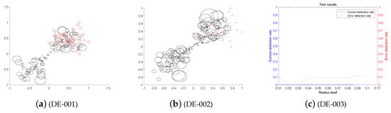
Figure 1.
The entangled image and error of the differential evolution (DE) algorithm running 200 times.
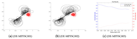
Figure 2.
The entangled image and error of the Differential Evolution Integration Algorithm Based on Mixed Penalty Function Screening Criteria (DE-MPFSC) algorithm running 200 times.
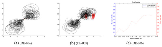
Figure 3.
The entangled image and error of the DE algorithm running 400 times.
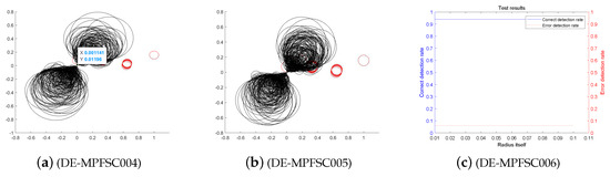
Figure 4.
The entangled image and error of the DE-MPFSC algorithm running 400 times.
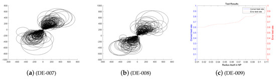
Figure 5.
The entangled image and error of the DE algorithm running 600 times.
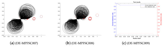
Figure 6.
The entangled image and error of the DE-MPFSC algorithm running 600 times.
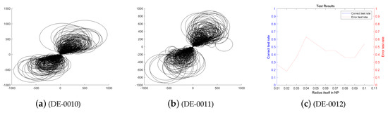
Figure 7.
The entangled image and error of the DE algorithm running 800 times.
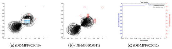
Figure 8.
The entangled image and error of the DE-MPFSC algorithm running 800 times.
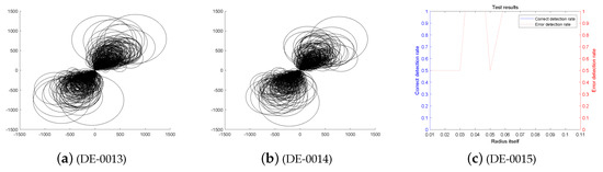
Figure 9.
The entangled image and error of the DE algorithm running 1000 times.
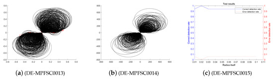
Figure 10.
The entangled image and error of the DE-MPFSC algorithm running 1000 times.
Figure 1, Figure 2, Figure 3, Figure 4, Figure 5, Figure 6, Figure 7, Figure 8, Figure 9 and Figure 10 above present entanglement degree analysis about the stability and validity between convergence precision and convergence speed of population individuals.
First, we analyze the stability and effectiveness of the DE-MPFSC algorithm from the number of population individuals. When the number of individuals are 200, 400, 600, 800, 1000, the DE algorithm entanglement degree about convergence precision and convergence speed are divided into two branches. However, the convergence speed and convergence precision are higher discrete and they do not converge to the entanglement center point along the convergence curve. The error test rates are 0.1, 0.65, 0.65, 0.55, 1, the correct test rate is 0 and the detection efficiency is 0, which shows that when the population individuals are 200, 400, 600, 800, 1000, the stability of the DE algorithm is not high and it is easy to generate fluctuations. Compared with the DE algorithm, the entanglement degree of the DE-MPFSC algorithm about convergence precision and convergence speed are divided into two branches. The convergence speed and convergence precision are lower discrete and they converge to the entanglement center point along the convergence curve. The error test rates are 0.25, 0.05, 0.05, 0.05, 0.05, the correct test rate are 0.75, 0.95, 0.95, 0.95, 0.95 and the detection efficiency are 3, 19, 19, 19, 19, which shows that when the population individuals are 200, 400, 600, 800, 1000, the stability of the DE-MPFSC algorithm is higher than DE algorithm.
In particular, when the number of individuals is 1000, the convergence speed and convergence precision are slightly lower than that of 800 individuals but the distribution is still scattered. They generate a more dramatic marginal differentiation phenomenon on branches and they do not converge to the entanglement center point along the convergence curve. The error test rate is 1, the correct test rate is 0 and the detection efficiency is 0. The situation must not be used as a basis for effective convergence, which shows that when the population individuals is 1000, the stability of the DE algorithm cannot be accepted and it is easy to generate fluctuations. Compared with the DE algorithm, the entanglement degree of the DE-MPFSC algorithm is divided into two branches. The convergence speed and convergence precision are lower discrete, which can further weak marginal differentiation phenomenon on branches and they converge to the entanglement center point along the convergence curve.
In summary, the stability of the DE-MPFSC algorithm is higher than that of the DE algorithm.
5.3. Numerical Test and Analysis of DE-MPFSC Algorithm
Since the data integration is closely related to the data size and data dimension, we set the population individuals to 1000, which is divided into 5 experiments and the average operation is 5 times for each experiment. According to the recommendations of Professor Storn R and Professor Price in Reference [19], the initial mutation factor and initial crossover probability are set to . Table 1, Table 2, Table 3, Table 4 and Table 5 below shows the numerical effects of (Differential Evolution Algorithm Based on Mixed Penalty Function Screening Criteria)DE-MPFSC algorithm and (Differential Evolution)DE algorithm.

Table 1.
Numerical Analysis of Entanglement Degree and Entanglement Degree Error of the Differential Evolution (DE) algorithm and the Mixed Penalty Function Screening Criteria (DE-MPFSC) algorithm 200 times.
Table 2.
Numerical Analysis of Entanglement Degree and Entanglement Degree Error of the DE algorithm and the DE-MPFSC algorithm 400 times.
Table 3.
Numerical Analysis of Entanglement Degree and Entanglement Degree Error of the DE algorithm and the DE-MPFSC algorithm 600 times.
Table 4.
Numerical Analysis of Entanglement Degree and Entanglement Degree Error of the DE algorithm and the DE-MPFSC algorithm 800 times.
Table 5.
Numerical Analysis of Entanglement Degree and Entanglement Degree Error of the DE algorithm and the DE-MPFSC algorithm 1000 times.
The above five data sheets in Table 1, Table 2, Table 3, Table 4 and Table 5 are data analysis of the entanglement degree , entanglement degree error and error rate about convergence precision and convergence speed. We experimented with 200 individuals as the cardinal number, repeating five times per experiment. We record the entanglement degree , entanglement degree error and error rate about DE algorithm and DE-MPFSC algorithm in real time. At the same time, we record the dynamic mutation factor F and the dynamic crossover probability of the DE-MPFSC algorithm and analyze the data tables one by one.
In summary, when the number of individuals is 200, 400, 600, 800 or 1000, the range of entanglement error rate of the DE algorithm and the DE-MPFSC algorithm are respectively and , which shows that the entanglement degree of the DE-MPFSC algorithm is significantly higher than that of the DE algorithm, and the stability of the DE-MPFSC algorithm is better. The range of entanglement degree of the DE algorithm and the DE-MPFSC algorithm are respectively and , which shows that the entanglement degree of the DE-MPFSC algorithm is significantly higher than that of the DE algorithm, and the fluctuation of the DE-MPFSC algorithm is lower. The entanglement error ranges of the DE algorithm and the DE-MPFSC algorithm are respectively and , which shows that the entanglement degree of the DE-MPFSC algorithm is significantly higher than that of the DE algorithm, and the DE-MPFSC convergence of the algorithm is stronger. In addition, there IS an additional discovery during the experiment that the optimal dynamic mutation factor and the optimal dynamic crossover probability of the DE-MPFSC algorithm are and respectively.
In summary, the convergence, stability and effectiveness of the DE-MPFSC algorithm are higher than the DE algorithm, which has obvious advantages for the integration of individuals.
5.4. Test and Analysis of DE-MPFSC Algorithm about Several Classic DE Algorithms
5.4.1. Entanglement Degree Test of DE-MPFSC Algorithm about Several Classic DE Algorithms
We choose four classic DE improved algorithms JDE, OBDE, DEGL and SADE for related tests. Through entanglement degree test and data analysis, we can verify the related performance of the DE-MPFSC algorithm and its superiority in data integration. From the previous experiments, we can know that the DE-MPFSC is better than the DE in stability, effectiveness and convergence. At the same time, the optimal dynamic mutation factor and the optimal crossover probability of the DE-MPFSC algorithm were obtained through data experiments. In the following test experiments, we use them as the initial mutation factor and the initial cross probability to better compare with other classic DE algorithms. Because the function of data integration is closely related to the data size and dimension, the algorithm in this paper sets the number of individuals to 1000 and are divided into 5 experiments. The number of individuals gradually increases in each test and the test runs an average of 4 times. We record relevant experimental indicators: dynamic mutation probability F, dynamic cross probability , entanglement degree , entanglement error , error rate , average individual loss efficiency. Figure 11, Figure 12, Figure 13, Figure 14 and Figure 15 below shows a numerical results of the experiment.
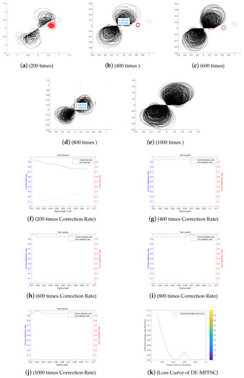
Figure 11.
The Entanglement Degree, Correction Rate and Loss Curve of DE-MPFSC algorithm.
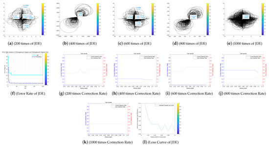
Figure 12.
The Entanglement Degree, Correction Rate and Loss Curve of the (Self-Adapting Parameter Setting in Differential Evolution) JDE algorithm.
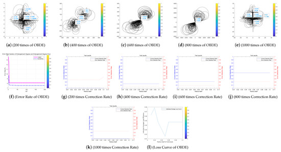
Figure 13.
The Entanglement Degree, Correction Rate and Loss Curve of the Opposition Based Differential Evolution (OBDE) algorithm.
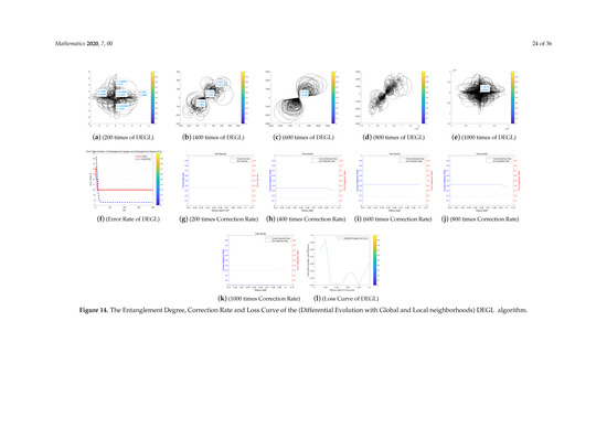
Figure 14.
The Entanglement Degree, Correction Rate and Loss Curve of the (Differential Evolution with Global and Local neighborhoods) DEGL algorithm.
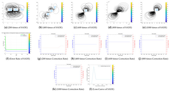
Figure 15.
The Entanglement Degree, Correction Rate and Loss Curve of the (Self-Adaptive Differential Evolution) SADE algorithm.
We analyze the above Figure 11, Figure 12, Figure 13, Figure 14 and Figure 15. First we analyze from the entanglement degree. In the process of the DE-MPFSC algorithm, the convergence speed and convergence precision of population individuals gradually stabilized as the population increased. The density and integration of the two entangled images gradually increase and, at the same time, the edge differentiation phenomenon is further weakened on each branch, which make the entangled branch converge to the center of the entanglement along the convergence curve. Compared with the DE-MPFSC algorithm, the entanglement phenomenon of the convergence speed and convergence precision of the JDE algorithm is less obvious. When the number of individuals is 200, 600 and 1000, the entangled image is highly dispersed, which causes a severe edge differentiation on the entangled branches. Although, when the number of individuals is 400 and 600, the state of entanglement is better than that of 200, 600 and 800, the continuity of individual evolution is not reached as a whole, it does not converge to the center of entanglement along the convergence curve. JDE’s entangled image shows irregular fluctuations. The OBDE algorithm is slightly better than the JDE algorithm in fluctuation, when the number of individuals is 200 and 1000, the entangled branches are severely differentiated and the dispersed degree is higher than that of JDE, which shows that the OBDE algorithm is not suitable. When the number of individuals is 400, 600 and 800, the dispersed degree of the entangled branches of the OBDE algorithm is lower but the edge dispersion of the entangled branches is more obvious than the DE-MPFSC algorithm. OBDE and JDE algorithms also do not show evolutionary continuity. The performance of the DEGL algorithm on evolutionary fluctuation is weaker than JDE and OBDE. When the number of individuals is 200 and 1000, the entangled branches are highly dispersed and do not converge to the entangled center. The DEGL is similar to the JDE algorithm and the OBDE algorithm. The individual convergence speed and convergence accuracy completely deviate from the entanglement center. The number of entangled branches integrated with 400 and 800 individuals is much higher than that with 200 and 1000 individuals. Although DEGL converges to the center of entanglement along the convergence curve, the edge differentiation of entangled branches is still not resolved. The continuity, volatility and convergence of the SADE algorithm are the closest to the DE-MPFSC algorithm but, unfortunately, a discrete state occurs when the number of individuals is 200, which makes the entanglement center distributed on the fitted line rather than an entanglement center. When the number of individuals is 400, 600, 800 and 1000, the edge dispersion of the entangled branches is weakened but it is not used for large-scale evolution.
Then we analyze from the correct test rate of entangled branches. The entanglement degree of the DE-MPFSC algorithm is divided into two branches about convergence precision and convergence speed. From the image, the convergence speed and convergence precision are lower discrete and they converge to the entanglement center point along the convergence curve. The detection efficiency are 3, 19, 19, 19, 19, which shows that when the population individuals are 200, 400, 600, 800, 1000, the stability of the DE-MPFSC algorithm is higher. Due to the fluctuation of the JDE algorithm, its correct test rate is 0, and its error test rates are 0.4, 0.4, 0.95, 0.6 and 0.95, respectively. JDE’s higher error test rate is easy to eliminate optimal individuals. The OBDE algorithm is weaker than the JDE algorithm in fluctuation. Its correct test rate is 0 but its error test rates are 1, 1, 0.4, 0.4, 1, which are higher than that of the JDE algorithm. When the number is 1000, the error test rate suddenly rebounds. The DEGL algorithm has a non-zero in correct test rate, which at least shows that there is a certain ability to adapt to individual mutations. But when the number of individuals is 200 and 1000, the error test rate of entangled branches is 1 and 0.95, which is still too high. When the number of individuals is 400 and 800, the correct test rate of entangled branches declines. The instability of this entanglement behavior is still not conducive to the evolution of mutation individuals. The correct test rate of the SADE algorithm are 0, 0, 0.35, 0.38, 0.35, and the error test rates are 0.4, 0.15, 0.15, 0.2, 0.15, which are much better than the JDE, OBDE and DEGL algorithms. Stability and continuity should be more conducive to the evolutionary behavior of large-scale individuals. However, compared to the DE-MPFSC algorithm, because of the correct test rate of the DEGL algorithm being too low, the detection of mutation individuals is not adaptive.
Finally, from the individual loss curve, we can know that the fluctuation of the JDE is higher than that of DE-MPFSC, OBDE, DEGL and SADE, indicating that during the individual evolution process, the population individual loss degree is higher. Especially for large-scale evolutionary populations, the risk of mutation individuals being lost during evolution will greatly increase. The individual loss degree of OBDE and DEGL rebounded in the later stages of evolution. The loss degree of mutation individuals showed an increasing trend relative to DE-MPFSC, JDE and SADE. The individual loss of SADE and DE-MPFSC is similar but the individual loss of SADE is higher than the latter. Because the individual losses of JDE, OBDE, DEGL and SADE are higher than DE-MPFSC, the advantages of the latter are obvious in stability. By analyzing the error rate curve, we can know that when DE-MPFSC is processing large-scale individuals (based on 200 individuals), the error rate of individual loss is lower than other algorithms.
5.4.2. Numerical Test of DE-MPFSC Algorithm about Several Classic DE Algorithms
We analyze the test results of the above data Table 6. We already know that when the number of individuals is 200, 400, 600, 800, 1000, the entanglement error range of DE-MPFSC is , The entanglement range of DE-MPFSC is , and the entanglement error range of DE-MPFSC is . When the number of individuals is 200, the entanglement error rate ranges of JDE, OBDE, DEGL and SADE are , , , , compared with DE-MPFSC, the former has a higher entanglement error rate, which shows that the entanglement degree of DE-MPFSC (since we have done a detailed analysis of the entanglement effect of the DE-MPFSC algorithm in the case of the same number of individuals, we will not repeat it here. For all comparative data, see Section 5.3) is significantly higher than that of JDE, OBDE, DEGL and SADE, and the algorithm has good stability and effectiveness. We also found a special case, when the number of individuals is 200, the entanglement degree and entanglement degree error of JDE, OBDE, DEGL are infinite or non-existent. The reason for the case is that the entangled branches are too discrete or the edges of the entangled branches are too severely differentiated. Obviously, their entanglement efficiency is significantly lower than DE-MPFSC. The entanglement range and entanglement error of SADE are and , , which is also lower than the entanglement effect of DE-MPFSC, which shows that the degree of entanglement of DE-MPFSC is significantly higher than that of JDE, OBDE, DEGL and SADE. The algorithm has small fluctuations and good convergence. When the number of individuals is 400, the entanglement error rate ranges of JDE, OBDE, DEGL and SADE are , , , , compared with DE-MPFSC, the entanglement error rate is higher, which shows that the degree of entanglement of DE-MPFSC is significantly higher than that of JDE, OBDE, DEGL and SADE, and the algorithm is better stability and effectiveness. The entanglement ranges of JDE, OBDE, DEGL and SADE are , , , , which shows that the degree of entanglement of the DE-MPFSC is significantly higher than that of JDE, OBDE, DEGL, SADE, and the DE-MPFSC algorithm has less volatility. The entanglement degree error ranges of JDE, OBDE, DEGL and SADE are , , , , which shows that the degree of entanglement of DE-MPFSC is significantly higher than that of JDE, OBDE, DEGL and SADE, and the algorithm has strong convergence. When the number of individuals is 600, 800, 1000, the comparison between DE-MPFSC and JDE, OBDE, DEGL and SADE is similar, and the data has been marked in the Table 6. On the whole, the effectiveness, stability, and convergence of DE-MPFSC are higher than JDE, OBDE, DEGL and SADE on average.
Table 6.
Numerical Analysis of Entanglement Degree and Entanglement Degree Error of the DE algorithm and the DE-MPFSC algorithm Several Times.
Then, we analyze from the state of entangled branches. When the number of individuals is 200, 400 or 1000, the entanglement degree and entanglement degree error of JDE do not exist, and the entanglement branches are in a discrete state. As the number of individuals increases, the entanglement effect appears fluctuating. When the number of individuals is 200 or 1000, the entanglement degree and entanglement degree error of OBDE do not exist, and the entangled branches are in a discrete state. When the number of individuals is 200, 400, 600 or 800, the integration of entangled branches gradually increases. However, the increase of OBDE is weaker than that of DE-MPFSC. The entanglement of the former shows a coexistence state of gradualism and fluctuation. When the number of individuals is 200 or 1000, the entanglement degree and entanglement degree error of DEGL do not exist, and the entangled branches are in a discrete state. When the number of individuals is 400 and 800, the integration of entangled branches begins to appear and it reaches the best state when the number of individuals is 600. The entanglement of DEGL shows coexistence of symmetry and fluctuation. The case is not conducive to the stable development of population evolution. When the number of individuals gradually increases, the entanglement degree and entanglement degree error of SADE are always integrated and increase with the number of individuals. However, due to the dispersion of the edges of the entangled branches, the entanglement increases slowly. Overall, DE-MPFSC has better stability and effectiveness than JDE, OBDE, DEGL and SADE.
6. Empirical Analysis
6.1. Verification Data Sets
We consider the imbalanced datasets, the UCI machine learning datasets [51] (the UCI Machine Learning Database is available at the following URL. https://archive.ics.uci.edu/ml/index.php), as integrated datasets to test the practical application level of the DE-MPFSC algorithm. First, we select three types of testing data from the UCI machine learning datasets, which are numerical value datasets (N.V. datasets), classify value datasets (C.V. datasets) and mixed value datasets(M.V. datasets). At the same time, according to the data integration level, the above three types of datasets are divided into level I, level II and level III, their proportions are 1, 2 and 3, respectively. The specific information on the three types of datasets is shown in Table 7.
Table 7.
The situation description of various types of data about the UCI machine learning datasets.
In this experiment, we divided the three types of data integration into single-link data integration (SLCE) and complete-link data integration (CLCE) according to the DE-MPFSC algorithm. The results obtained by the two integrated methods are compared with the results obtained by the KNN-SK (KNN data filling) [52,53,54] and the SKNN-SK (SKNN data filling) [52,53,54]. To ensure that there is single-random for the data in Table 1, we performed random deletion in a five percent ratio on the computer. Then, we conducted the algorithm test and obtained the results by performing the test 200 times on the computer in the same integrated method for the same datasets.
6.2. Verification Indicator
To interpret the effect of the DE-MPFSC algorithm on the imbalanced data integrated and classified, we need to verify the consistency of the imbalanced data. First, we should establish the verification indicator of classification accuracy (CA) [55,56], adjusted rand index (ARI) [55,56], normalized mutual information (NMI) [55,56] to test the effect of the DE-MPFSC algorithm, which are described as follows.
(1) CA: CA is a statistical mathematics variable measuring the imbalanced data samples proportion of the DE-MPFSC algorithm in making up for data integrated defects, which is expressed as follows.
where is a subsample of the DE-MPFSC algorithm in making up for data integrated defects, k is the number of integrated classes, n is the sample capacity.
(2) ARI: ARI is a statistical mathematics variable measuring the imbalanced data samples proportion of the DE-MPFSC algorithm in making up for data integrated defects after considering the same data class and different data classes, which is expressed as follows.
(3) NMI: NMI is a similarity variable measuring sample data and integrated data after comparing and correctly integrating and classing imbalanced data within being integrated defects, which is expressed as follows.
where is the sample size in the data integrated result where the ith datasets contains the original datasets j. is the sample size of the ith datasets in the data integrated result. is the sample size of the original datasets j. n is the samples. is the number of different types of datasets and the number of original datasets obtained in the data integrated result. The limit value of the three types of verification indicators is set to 1. If the data structure is close to the original data structure after imbalanced integrated data, which means that the value of the dataset is larger compared to the original datasets. That is, the DE-MPFSC algorithm has a better effect on imbalanced data integration.
6.3. The Test Analysis
The number of neighbors selected by the KNN-SK and SKNN-SK is . The testing results of the (Differential Evolution Algorithm Based on Mixed Penalty Function Screening Criteria)DE-MPFSC algorithm and other algorithms under the verification indicators are shown in Table 8 and Figure 16, Figure 17 and Figure 18 about Classification Accuracy , Adjusted Rand Index , and Normalized Mutual Information datasets.
Table 8.
Data integration Comparison about CA, NMI and ARI Values of the DE-MPFSC Algorithm.

Figure 16.
Convergence integration of DE-MPFFC algorithm for CA.
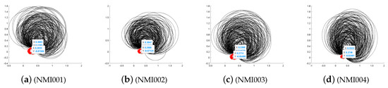
Figure 17.
Convergence integration of DE-MPFFC algorithm for NMI.
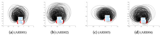
Figure 18.
Convergence integration of DE-MPFFC algorithm for ARI.
Where according to the data analysis in Table 8, we know that since the single data integrated method KNN-SK and SKNN-SK do not have fitting characteristics inside the data integration and consistency are better than single integrated methods.
The CA value, ARI value and NMI value of UCI data about DE-MPFSC algorithm are as follows: the optimal value and sub-optimal value tend to distribution in probability 1, while the other data points tend to distribution in probability 0, in which the data points tended to distribution in probability 1 are in the feasible region and the data points tended to distribution in probability 0 are in the non-feasible region. The CA value, ARI value and NMI value of Credit Approval data about DE-MPFSC algorithm are as follows: the optimal value and sub-optimal value tend to distribution in probability 1, while the other data points tend to distribution in probability 0, in which the data points tended to distribution in probability 1 are in the feasible region and the data points tended to distribution in probability 0 are in the non-feasible region. For the data (CMC) and Glass marked with ■, the values of CA, ARI and NMI are as follows: the optimal value and the sub-optimal value are stable around the probability of 0.5, and the error does not exceed , which accord with the stability requirements of data.
The CA value, ARI value and NMI value of all data about DE-MPFSC algorithm are as follows: the average optimal value and the average sub-optimal quality are stable around the probability of 0.5 and the error does not exceed . The variance optimal value and the variance sub-optimal value are basically stable around 0.01, which accord with the data stability standard and the error does not exceed 0.0001.From the datasets in Table 8, the optimal value of the DE-MPFSC algorithm in both mean and variance shows the superiority of the algorithm.
It can be seen from the Figure 16, Figure 17 and Figure 18 that through the two-dimensional reduced order analysis of UCI machine learning data, it is found that the three data integration effects of , and show a trend of highly integrated convergence within an acceptable error range.
First, we analyze from the precision. The integration effect on CA data is as follows: the minimum upper bound of the reduced-order 2D data in the X direction is and the error does not exceed . The maximum lower bound of the reduced-order 2D data in the Y direction is and the error does not exceed . The entanglement error of the imbalanced data set in both X and Y directions is . It can be seen that the precision in both directions of X and Y is in a fully controllable and highly integrated range, which fully shows that the DE-MPFSC algorithm has a good integration advantage for improving the integration accuracy of CA data. The integration effect on NMI data is as follows—the minimum upper bound of the reduced-order 2D data in the X direction is and the error does not exceed . The maximum lower bound of the reduced-order 2D data in the Y direction is and the error does not exceed . The entanglement error of the imbalanced data set in both X and Y directions is . It can be seen that the precision in both directions of X and Y is in a fully controllable and highly integrated range, which fully demonstrates that the DE-MPFSC algorithm has a good integration advantage for improving the integration accuracy of NMI data. The integration effect on ARI data is as follows: the minimum upper bound of the reduced-order 2D data in the X direction is and the error does not exceed . The maximum lower bound of the reduced-order 2D data in the Y direction is and the error does not exceed . The entanglement error of the imbalanced data set in both X and Y directions is . It can be seen that the precision in both directions of X and Y is in a fully controllable and highly integrated range, which fully shows that the DE-MPFSC algorithm has a good integration advantage for improving the integration accuracy of ARI data.
Then we analyze the density of data integration. The integration effect on CA data is as follows: The integration curve integrated with as the center. The entanglement error is and the integration curve radius is . The data integration density is higher than before, and the imbalanced data that presents the red part and the balanced data that presents the black part are completely separated, which fully shows that the DE-MPFSC algorithm has a better distribution advantage for improving the accuracy of CA data integration. The integration effect on NMI data is as follows: The integration curve integrated with as the center. The entanglement error is and the integration curve radius is . The data integration density is higher than before, and the imbalanced data that presents the red part and the balanced data that presents the black part are completely separated, which fully shows that the DE-MPFSC algorithm has a better distribution advantage for improving the accuracy of NMI data integration. The integration effect on ARI data is as follows: The integration curve integrated with as the center. The entanglement error is and the integration curve radius is . The data integration density is higher than before and the imbalanced data that presents the red part and the balanced data that presents the black part are completely separated, which fully shows that the DE-MPFSC algorithm has a better distribution advantage for improving the accuracy of ARI data integration.
Finally, we analyze the degree of data separation. From the distribution of Figure 16, Figure 17 and Figure 18, CA data, NMI data and ARI data have been completely separated by the DE-MPFSC algorithm. The data integration effect presents the following trend: the data set that is balanced is in the black curve part and tends to converge toward the center of the integration curve, and the imbalanced data set is in the red curve part and tends to converge toward the center of the integration curve.
The above analysis shows that the DE-MPFSC algorithm has a good natural advantage in integrating imbalanced data.
7. Conclusions
In this paper, some processing problems of imbalanced data. We design the algorithm based on the DE algorithm, constructs a differential evolution algorithm based on a mixed penalty function screening criterion for imbalanced data integration. The method can improve the classification problem of imbalanced data and construct an empirical analysis through UCI machine learning datasets. In addition, the verification result is in accordance with the imbalanced data classification expectation and the integration effect. The main work of this article is as follows:
1. Based on the normalization of internal and external penalty functions, we established the mixed penalty function screening criteria on DE algorithm.
2. We established a differential evolution integration algorithm (DE-MPFSC algorithm) based on the mixed penalty function screening criterion, which broadens the algorithm foundation for the efficient integration of imbalanced data.
3. We constructed the Markov process of the DE-MPFSC algorithm and proved the theoretical validity and evolution mechanism of DE-MPFSC algorithm.
4. We creatively introduce the entanglement and entanglement error and compare the performance of the DE-MPFSC algorithm through data analysis.
5. Based on the empirical analysis of the UCI machine learning data, we further illustrated the effectiveness of the DE-MPFSC algorithm in the efficient integration of the imbalanced data, leading to multimode imbalanced data integration.
Author Contributions
Y.G. provided the research ideas of the paper; K.W. solved the overall framework, algorithm framework, paper structure, and result analysis of the research ideas of the paper; C.G. provides data analysis and corresponding analysis results; Y.S. provides the overall research ideas and main methods of the paper; T.L. has helped the writing of the paper.
Funding
This work was supported by the Major Scientific Research Special Projects of North Minzu University (No.ZDZX201901), the NSFC (No.61561001;11961001), Graduate Innovation Project of North Minzu University (No:YCX19120), First-Class Disciplines Foundation of Ningxia (No:NXYLXK2017B09) and the by National Natural Science Foundation of Shanxi Province (2019JM-425), China Postdoctoral Science Foundation Funded Project (2019M653567).
Acknowledgments
Acknowledgment for the financial support of the National Natural Science Foundation Project, the University-level Project of Northern University for Nationalities and the District-level Project of Ningxia, the Major Scientific Research Special Projects of North Minzu University and all authors’ efforts. And the reviewers and instructors for the paper.
Conflicts of Interest
The authors declare no conflict of interest.
References
- Everitt, B. Cluster Analysis. Qual. Quant. 1980, 14, 75–100. [Google Scholar] [CrossRef]
- Chunyue, S.; Zhihuan, S.; Ping, L.; Wenyuan, S. The study of Naive Bayes algorithm online in data mining. In Proceedings of the World Congress on Intelligent Control and Automation, Hangzhou, China, 15–19 June 2004. [Google Scholar]
- Samanta, B.; Al-Balushi, K.R.; Al-Araimi, S.A. Artificial neural networks and genetic algorithm for bearing fault detection. Soft Comput. Fusion Found. Methodol. Appl. 2006, 10, 264–271. [Google Scholar] [CrossRef]
- Díez-Pastor, J.F.; Rodríguez, J.J.; García-Osorio, C.; Kuncheva, L.I. Random Balance: Ensembles of variable priors classifiers for imbalanced data. Knowl.-Based Syst. 2015, 85, 96–111. [Google Scholar] [CrossRef]
- Maldonado, S.; Weber, R.; Famili, F. Feature selection for high-dimensional class-imbalanced data sets using Support Vector Machines. Inf. Sci. 2014, 286, 228–246. [Google Scholar] [CrossRef]
- Chawla, N.V.; Bowyer, K.W.; Hall, L.O.; Kegelmeyer, W.P. SMOTE: Synthetic minority over-sampling technique. J. Artif. Intell. Res. 2002, 16, 321–357. [Google Scholar] [CrossRef]
- Vorraboot, P.; Rasmequan, S.; Chinnasarn, K.; Lursinsap, C. Improving classification rate constrained to imbalanced data between overlapped and non-overlapped regions by hybrid algorithms. Neurocomputing 2015, 152, 429–443. [Google Scholar] [CrossRef]
- Krawczyk, B.; Woźniak, M.; Schaefer, G. Cost-sensitive decision tree ensembles for effective imbalanced classification. Appl. Soft Comput. 2014, 14, 554–562. [Google Scholar] [CrossRef]
- López, V.; Río, S.D.; Benítez, J.M.; Herrera, F. Cost-sensitive linguistic fuzzy rule-based classification systems under the MapReduce framework for imbalanced big data. Fuzzy Sets Syst. 2015, 258, 5–38. [Google Scholar] [CrossRef]
- Santucci, V.; Milani, A.; Caraffini, F. An Optimisation-Driven Prediction Method for Automated Diagnosis and Prognosis. Mathematics 2019, 7, 1051. [Google Scholar] [CrossRef]
- Mikalef, P.; Boura, M.; Lekakos, G.; Krogstie, J. Big data analytics and firm performance: Findings from a mixed-method approach. J. Bus. Res. 2019, 98, 261–276. [Google Scholar] [CrossRef]
- Thai-Nghe, N.; Gantner, Z.; Schmidt-Thieme, L. Cost-sensitive learning methods for imbalanced data. In Proceedings of the International Joint Conference on Neural Networks, Barcelona, Spain, 18–23 July 2010; pp. 1–8. [Google Scholar]
- Freund, Y. Boosting a weak learning algorithm by majority. Inf. Comput. 1995, 121, 256–285. [Google Scholar] [CrossRef]
- Breiman, L. Bagging predictors, machine learning research: Four current directors. ResearchGate 1996, 24, 123–140. [Google Scholar]
- Sun, Z.; Song, Q.; Zhu, X.; Sun, H.; Xu, B.; Zhou, Y. A novel ensemble method for classifying imbalanced data. Pattern Recognit. 2015, 48, 1623–1637. [Google Scholar] [CrossRef]
- Chawla, N.V.; Lazarevic, A.; Hall, L.O.; Bowyer, K.W. SMOTEBoost: Improving Prediction of the Minority Class in Boosting. Knowledge Discovery in Databases: Pkdd 2003. In Proceedings of the European Conference on Principles and Practice of Knowledge Discovery in Databases, Cavtat-Dubrovnik, Croatia, 22–26 September 2003; pp. 107–119. [Google Scholar]
- Flach, P.A.; Lachiche, N. Naive Bayesian Classification of Structured Data. Mach. Learn. 2004, 57, 233–269. [Google Scholar] [CrossRef]
- Fernández, A.; López, V.; Galar, M.; Del Jesus, M.; Herrera, F. Analysing the classification of imbalanced data-sets with multiple classes: Binarization techniques and ad-hoc approaches. Knowl.-Based Syst. 2013, 42, 97–110. [Google Scholar] [CrossRef]
- Storn, R.; Price, K. Differential Evolution—A Simple and Efficient Heuristic for global Optimization over Continuous Spaces. J. Glob. Optim. 1997, 11, 341–359. [Google Scholar] [CrossRef]
- Wang, K.; Gao, Y. Topology Structure Implied in β-Hilbert Space, Heisenberg Uncertainty Quantum Characteristics and Numerical Simulation of the DE Algorithm. Mathematics 2019, 7, 330. [Google Scholar] [CrossRef]
- Das, S.; Mullick, S.S.; Suganthan, P.N. Recent advances in differential evolution—An updated survey. Swarm Evol. Comput. 2016. [Google Scholar] [CrossRef]
- Neri, F.; Tirronen, V. Recent advances in differential evolution: A survey and experimental analysis. Artif. Intell. Rev. 2010, 33, 61–106. [Google Scholar] [CrossRef]
- Das, S.; Suganthan, P.N. Differential Evolution: A Survey of the State-of-the-Art. IEEE Trans. Evol. Comput. 2011, 15, 4–31. [Google Scholar] [CrossRef]
- Brest, J.; Zumer, V.; Maucec, M.S. Self-Adaptive Differential Evolution Algorithm in Constrained Real-Parameter Optimization. In Proceedings of the IEEE Congress on Evolutionary Computation (CEC 2006), Vancouver, BC, Canada, 16–21 July 2006. [Google Scholar]
- Brest, J.; Zamuda, A.; Bošković, B.; Greiner, S.; Zumer, V. An Analysis of the Control Parameters’ Adaptation in DE. Stud. Comput. Intell. 2008. [Google Scholar] [CrossRef]
- Rahnamayan, S.; Tizhoosh, H.R.; Salama, M.M.A. Opposition-based differential evolution. IEEE Trans. Evol. Comput. 2008, 12, 64–79. [Google Scholar] [CrossRef]
- Das, S.; Abraham, A.; Chakraborty, U.K.; Konar, A. Differential Evolution Using a Neighborhood-Based Mutation Operator. IEEE Trans. Evol. Comput. 2009, 13, 526–553. [Google Scholar] [CrossRef]
- Mallipeddi, R.; Suganthan, P.N. Ensemble of Constraint Handling Techniques. IEEE Trans. Evol. Comput. 2010, 14, 561–579. [Google Scholar] [CrossRef]
- Qu, B.Y.; Suganthan, P.N. Constrained multi-objective optimization algorithm with an ensemble of constraint handling methods. Eng. Optim. 2011, 43, 403–416. [Google Scholar] [CrossRef]
- Qin, A.K.; Suganthan, P.N. Self-adaptive differential evolution algorithm for numerical optimization. In Proceedings of the IEEE Congress on Evolutionary Computation (CEC 2005), Edinburgh, UK, 2–4 September 2005. [Google Scholar]
- Zou, D.; Liu, H.; Gao, L.; Li, S. A modified differential evolution algorithm for unconstrained optimization problems. Neurocomputing 2011, 120, 1608–1623. [Google Scholar] [CrossRef]
- Ghosh, A.; Das, S.; Chowdhury, A.; Giri, R. An improved differential evolution algorithm with fitness-based adaptation of the control parameters. Inf. Sci. 2011, 181, 3749–3765. [Google Scholar] [CrossRef]
- Caraffini, F.; Kononova, A.V.; Corne, D. Infeasibility and structural bias in Differential Evolution. Inf. Sci. 2019, 496, 161–179. [Google Scholar] [CrossRef]
- Storn, R. System design by constraint adaptation and differential evolution. IEEE Trans. Evol. Comput. 1999, 3, 22–34. [Google Scholar] [CrossRef]
- Thomsen, R. Flexible ligand docking using differential evolution. In Proceedings of the 2003 Congress on Evolutionary Computation (CEC ’03), Canberra, Australia, 8–12 December 2003; Volume 4, pp. 2354–2361. [Google Scholar]
- Ali, M.; Pant, M.; Singh, V.P. An improved differential evolution algorithm for real parameter optimization problems. Int. J. Recent Trends Eng. 2009, 1, 63–65. [Google Scholar]
- Yang, M.; Li, C.; Cai, Z.; Guan, J. Differential evolution with auto-enhanced population diversity. IEEE Trans. Cybern. 2015, 45, 302–315. [Google Scholar] [CrossRef] [PubMed]
- Iri, M.; Imai, H. Theory of the multiplicative penalty function method for linear programming. Discret. Algorithms Complex. 1987, 30, 417–435. [Google Scholar]
- Rao, S.S.; Bard, J. Engineering Optimization: Theory and Practice, 4th ed.; A I I E Transactions; John Wiley & Sons: New York, NY, USA, 1997; Volume 29, pp. 802–803. [Google Scholar]
- Wright, M. The interior-point revolution in optimization: History, recent developments, and lasting consequences. Bull. Am. Math. Soc. 2005, 42, 39–57. [Google Scholar] [CrossRef]
- Deb, K. An efficient constraint handling method for genetic algorithms. Comput. Methods Appl. Mech. Eng. 2000, 186, 311–338. [Google Scholar] [CrossRef]
- Venkatraman, S.; Yen, G.G. A Generic Framework for Constrained Optimization Using Genetic Algorithms; IEEE Press: Piscataway, NJ, USA, 2005. [Google Scholar]
- Xie, X.F.; Zhang, W.J.; Bi, D.C. Handling equality constraints by adaptive relaxing rule for swarm algorithms. In Proceedings of the 2004 Congress on Evolutionary Computation (IEEE Cat. No.04TH8753), Portland, OR, USA, 19–23 June 2004; Volume 2. [Google Scholar]
- Schwefel, H.P. Evolution and Optimum Seeking; Wiley: New York, NY, USA, 1995. [Google Scholar]
- Kramer, O. Premature Convergence in Constrained Continuous Search Spaces. In Proceedings of the Parallel Problem Solving from Nature—PPSN X, Dortmund, Germany, 13–17 September 2008; Springer: Berlin/Heidelberg, Germany, 2008; pp. 62–71. [Google Scholar]
- Gasparini, M. Markov Chain Monte Carlo in Practice; Markov chain monte carlo in practice; Chapman and Hall: London, Uk, 1996; pp. 9236–9240. [Google Scholar]
- Eiben, A.E.; Aarts, E.H.L.; Hee, K.M.V. Global Convergence of Genetic Algorithms: A Markov Chain Analysis; Parallel Problem Solving from Nature; Springer: Berlin/Heidelberg, Germany, 1991; pp. 3–12. [Google Scholar]
- Rudolph, G. Convergence of evolutionary algorithms in general search spaces. In Proceedings of the IEEE International Conference on Evolutionary Computation, Nagoya, Japan, 20–22 May 1996; pp. 50–54. [Google Scholar]
- Cerf, R. Asymptotic Convergence of Genetic Algorithms. Adv. Appl. Probab. 1998, 30, 521–550. [Google Scholar] [CrossRef]
- Xu, Z.B.; Nie, Z.K.; Zhang, W.X. Almost sure strong convergence of a class of genetic algorithms with parent-offspring competition. Acta Math. Appl. Sin. 2002, 25, 167–175. [Google Scholar]
- Unified Communications Irvine Machine Learning Repository(UCI). Available online: https://archive.ics.uci.edu/ml/index.php (accessed on 1 August 2019).
- Silva, L.O.; Zárate, L.E. A brief review of the main approaches for treatment of missing data. Intell. Data Anal. 2014, 18, 1177–1198. [Google Scholar] [CrossRef]
- Batista, G.A.P.A. MariaCarolinaMonard. An analysis of four missing data treatment methods for supervised learning. Appl. Artif. Intell. 2003, 17, 519–533. [Google Scholar] [CrossRef]
- Liang, J.; Bai, L.; Dang, C.; Cao, F. The K-Means-Type Algorithms Versus Imbalanced Data Distributions. IEEE Trans. Fuzzy Syst. 2012, 20, 728–745. [Google Scholar] [CrossRef]
- Strehl, A.; Ghosh, J. Cluster ensembles—A knowledge reuse framework for combining multiple partitions. J. Mach. Learn. Res. 2002, 3, 583–617. [Google Scholar]
- Zhao, X.; Liang, J.; Dang, C. Clustering ensemble selection for categorical data based on internal validity indices. Pattern Recognit. 2017, 69, 150–168. [Google Scholar] [CrossRef]


© 2019 by the authors. Licensee MDPI, Basel, Switzerland. This article is an open access article distributed under the terms and conditions of the Creative Commons Attribution (CC BY) license (http://creativecommons.org/licenses/by/4.0/).