Construction of Cubic Timmer Triangular Patches and its Application in Scattered Data Interpolation

Abstract

This paper discusses scattered data interpolation by using cubic Timmer triangular patches. In order to achieve C¹ continuity everywhere, we impose a rational corrected scheme that results from convex combination between three local schemes. The final interpolant has the form quintic numerator and quadratic denominator. We test the scheme by considering the established dataset as well as visualizing the rainfall data and digital elevation in Malaysia. We compare the performance between the proposed scheme and some well-known schemes. Numerical and graphical results are presented by using Mathematica and MATLAB. From all numerical results, the proposed scheme is better in terms of smaller root mean square error (RMSE) and higher coefficient of determination (R²). The higher R² value indicates that the proposed scheme can reconstruct the surface with excellent fit that is in line with the standard set by Renka and Brown’s validation.

1. Introduction

Many computer graphics and vision problems involve scattered data interpolation (SDI). SDI methods aims to build a smooth function from a set of data, which consist of functional values corresponding to points, which do not obey any structure or order between their relative locations. These methods have a wide range of uses in surface reconstruction, visualization, image restoration, computer graphics, surface deformation, image processing, engineering, and technology, etc.

Most researchers have investigated surface interpolation based on triangulations of scattered data and there are several scattered data fitting techniques, such as the Delaunay triangulation method [1], radial basis function (RBF) [2], and moving least square (MLS) [3]. Very recently, new techniques for interpolating scattered data have been developed [1,4,5], which can be implemented in fast algorithms [6].

The most popular method that is usually used to generate the surface of scattered from the data points is Delaunay triangulation method [7]. It is a very famous method, applied to produce the triangle meshes, where vertices of the triangle are made up of the sample data points.

The property of shape preserving interpolation is an important technique usually applied in curve and surface modeling. Several research papers [2,7,8,9,10,11,12,13] have been published on shape preservation in the last couple of years. Ibraheem et al. [14] proposed a scheme that is suitable for surface reconstruction and deformation. The objective of the scheme is to develop a local positivity preserving when the data points are used.

A new big data infrastructure for the management of cultural items was proposed by Su et al. [15]. It is a multilayer architecture to create new applications based on the modules that were offered by APIs. Streams of data from social networks are mostly captured by this module to handle and update the information. They tested their system by created an application of the Android devices called the Smart Search Museum. This application will access the map that has all the museums of a given area in Italy. Nowadays, the demand for information monitoring and recommendation technology is getting bigger, which is suggested by the systems proposed by [1]. They proposed a novel, collaborative, and user-centered approach for big data application.

This study is an extension of the paper discussed by Ali et al. [16]. The main objective of this study is to construct the SDI using Timmer triangular patches, which are used to visualize the energy data i.e., spatial interpolation in visualizing rainfall data. Firstly, we triangulate the domain data using Delaunay triangulation. Next, we specify the derivatives at the data points and assign Timmer ordinate values for each triangular patch. Lastly, we generate the Timmer triangular patches of the surface. The main novelty of this work is that we construct new cubic triangular Timmer patches and apply them for scattered data interpolation. The proposed scheme has higher accuracy as well as requiring smaller CPU times (in seconds) than some existing schemes.

The rest of the paper is organized as follows. The method of the study is discussed in Section 2 including the derivation of cubic Timmer triangular patches with some examples. In Section 3, we discuss the derivation of the sufficient condition for $C^1$ continuity on all adjacent triangles. Numerical and graphical results including comparison with some established schemes are presented in Section 4. In the final section, some conclusions and recommendations for future studies are made.

2. Cubic Timmer Triangular Patches

Ali et al. [16] introduced a new cubic triangular basis function, which was actually the extension of the univariate cubic Timmer basis proposed by Timmer [17]. The new cubic Timmer triangular patch is different from the cubic Ball and cubic Bezier triangular patches [16].

The cubic Timmer patch is defined as follows [16]:

$$T\left(u,v,w\right)={\displaystyle \sum }_{i+j+k=3}{T}_{ijk}^3\left(u,v,w\right)t_{i,j,k}.$$

(1)

Equation (1) can be written as

$$\begin{array}{cc}\hfill T\left(u,v,w\right)=& u^2\left(2u-1\right)t_{300}+4u^{2}v{t}_{210}+4u^{2}w{t}_{201}\hfill \\ & +v^2\left(2v-1\right)t_{030}+4v^{2}u{t}_{120}+ 4v^{2}w{t}_{021}\hfill \\ & +w^2\left(2w-1\right)t_{003}+4w^{2}u{t}_{102}\hfill \\ & +4w^{2}v{t}_{012}+6uvw{t}_{111}\hfill \end{array}$$

(2)

where $t_{ijk}$ denotes the control point, while $T_{ijk}^3\left(u,v,w\right), i+j+k=3$ are cubic Timmer triangular basis functions defined in [16]. Some properties of the Timmer triangle patch described in Equation (1) are the following:

(a)

Partition of unity: The new cubic Timmer triangular basis satisfies:

$${\displaystyle \sum }_{i=0}^3{T}_{ijk}^3\left(u,v,w\right)=1.$$

(b)

Symmetry: The surfaces generated from two different ordering of its control points will look the same.

(c)

Positivity: In each of the cubic Timmer triangular basis functions, the positivity or nonnegativity behavior ${\mathit{T}}_{\mathit{i}\mathit{j}\mathit{k}}^{\mathbf{3}}\left(\mathit{u},\mathit{v},\mathit{w}\right)\ge \mathbf{0}$ is fulfilled, except for the following: ${\mathit{T}}_{\mathbf{300}}^{\mathbf{3}}\left(\mathit{u},\mathit{v},\mathit{w}\right)\le \mathbf{0}$ when $\frac{\mathbf{1}}{\mathbf{2}}\le \mathit{u}\le \mathbf{1}$ and both ${\mathit{T}}_{\mathbf{201}}^{\mathbf{3}}\left(\mathit{u},\mathit{v},\mathit{w}\right)\le \mathbf{0}$ and ${\mathit{T}}_{\mathbf{210}}^{\mathbf{3}}\left(\mathit{u},\mathit{v},\mathit{w}\right)\le \mathbf{0}$ when $\mathbf{0}\le \mathit{u}\le \frac{\mathbf{1}}{\mathbf{2}}$.

(d)

Convex hull: The Timmer triangular patches may not lie within the convex hull of the control polygon. If the positivity property is fulfilled for the Timmer triangular patches as discussed in (c), it will satisfy the convex hull property.

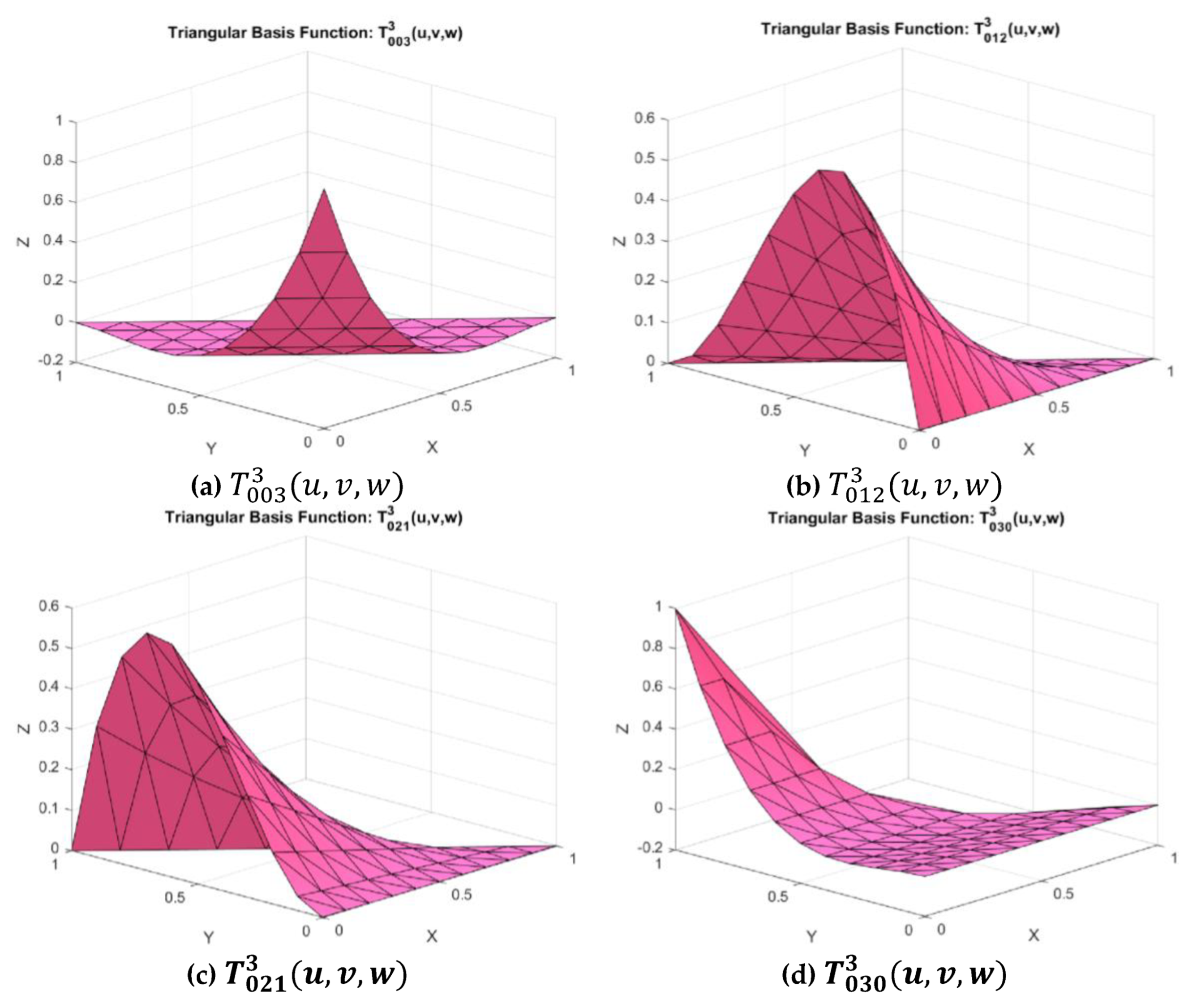
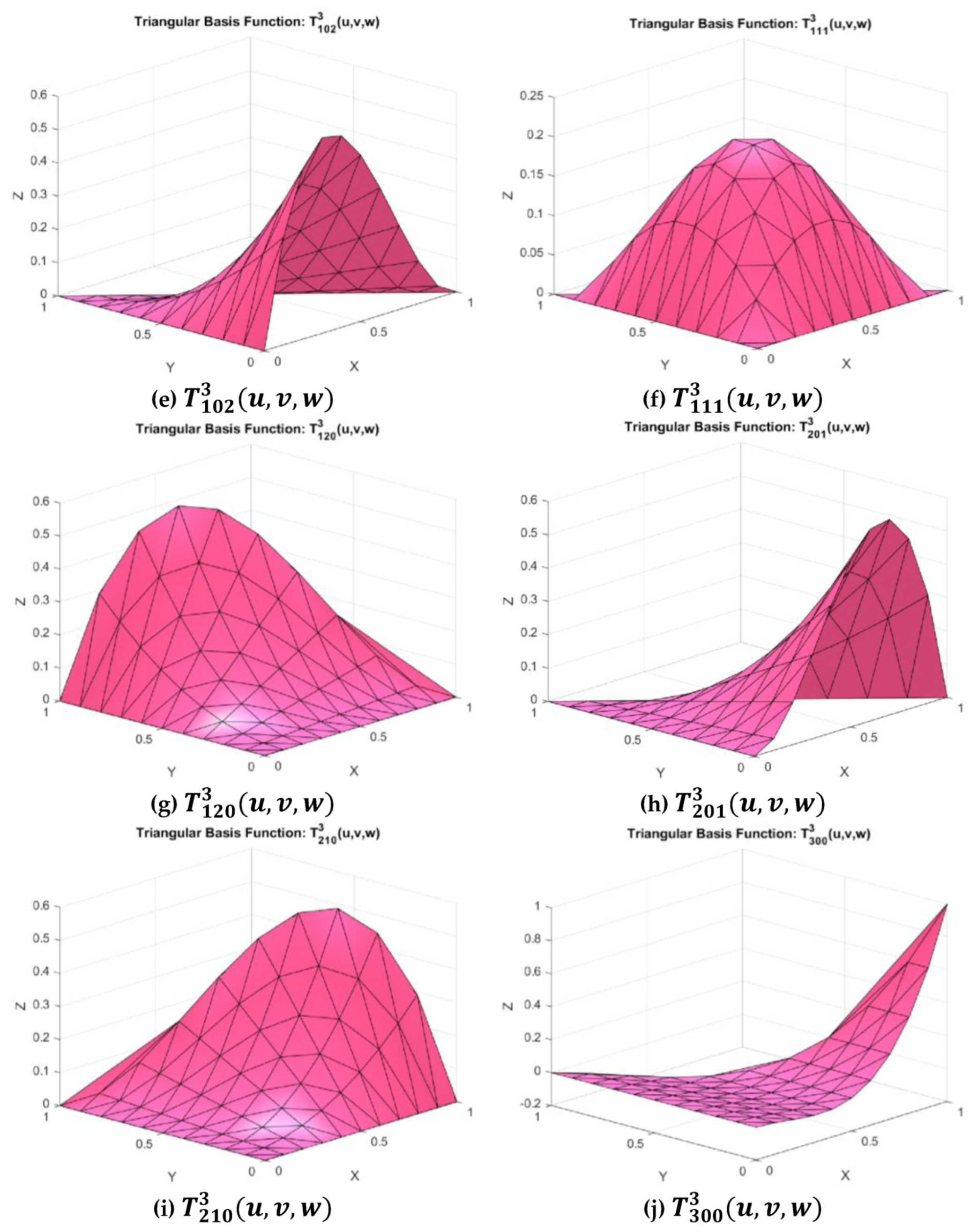
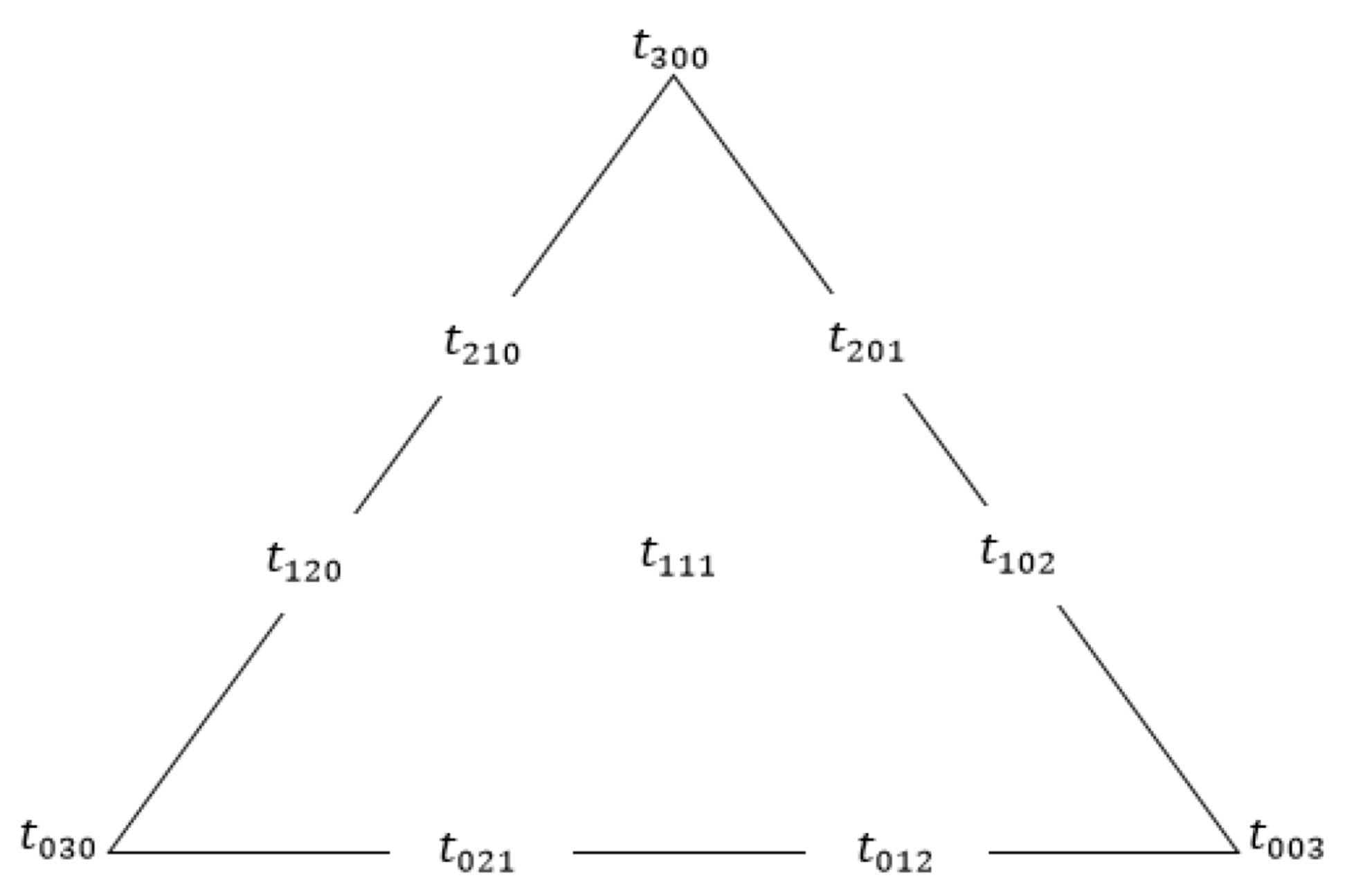
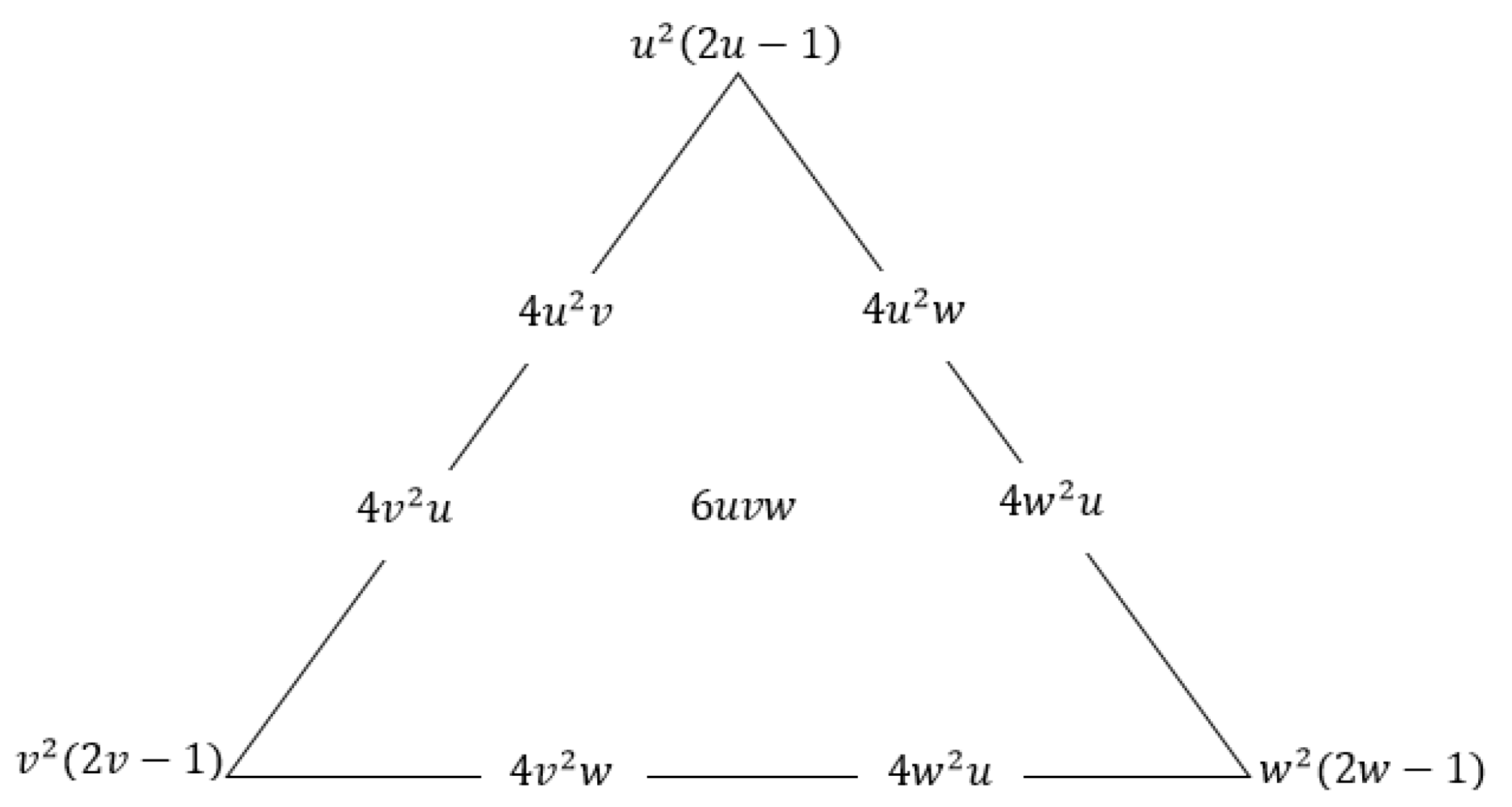
Figure 1, Figure 2 and Figure 3 show the cubic Timmer triangular basis functions, the Timmer ordinates for the cubic Timmer triangular patch, and the cubic Timmer triangular bases, respectively.

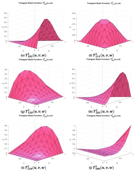
Figure 1. Some cubic Timmer triangular basis functions.

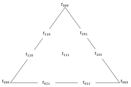
Figure 2. Control nets for cubic Timmer triangular patch.

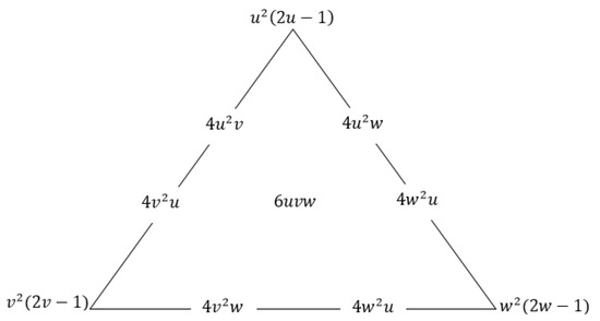
Figure 3. Cubic Timmer triangular bases.

Then, one set of control points is used to construct the surface of cubic Timmer triangular patch. Table 1 shows the control point used to construct the surfaces in Figure 4.

Table 1. Control points.

x	−4.0	−4.0	−4.0	−4.0	−1.5	1.0	3.5	1.0	−1.5	−1.5
y	3.5	1.0	−1.5	−4.0	−4.0	−4.0	−4.0	−1.5	−1.5	−1.5
z	20.25	9.00	1.0.25	24.00	10.25	9.00	20.25	4.75	4.75	3.50

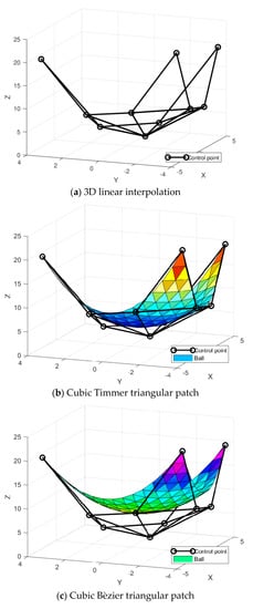
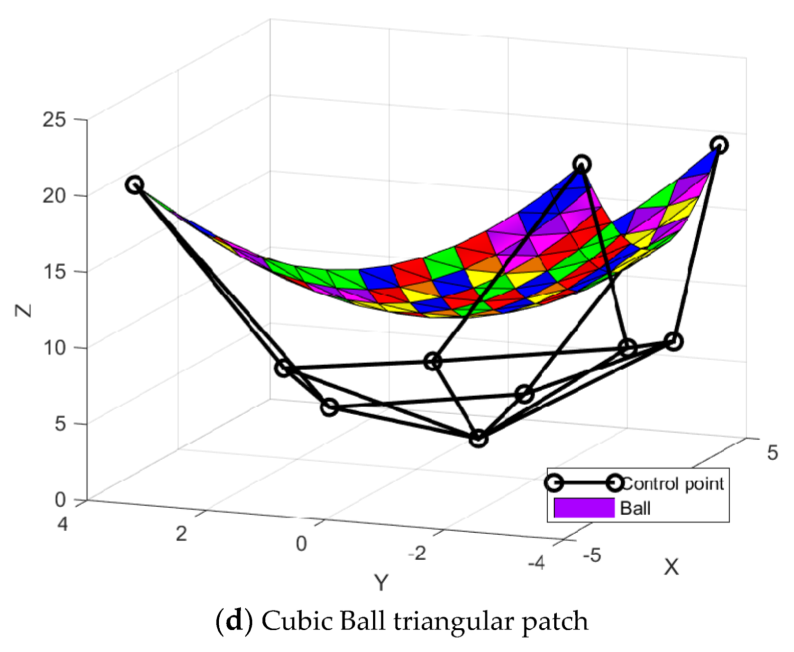
Figure 4. Surface interpolation.

It is observed from Figure 4 that cubic Timmer triangular patches lie in close vicinity of the control polygon as compared to cubic Bèzier and Ball triangular patches, respectively. The cubic Bèzier and Ball triangular patches satisfy the convex hull property while the cubic Timmer triangular, in general, does not obey the convex hull property. However, cubic Timmer triangular patches are close to the control polyhedron.

3. Derivation of Sufficient Condition for ${\mathit{C}}^{\mathbf{1}}$ Continuity on Adjacent Triangles

In this section, we show in detail the derivation of the sufficient condition that have been considered in Ali et al. [2]. The derivatives of $T$ with respect to the direction $s=\left(s_x,s_y,s_z\right)=s_x{V}_1+s_y{V}_2+s_z{V}_3,s_x+s_y+s_z=0$ are given by:

$$D_{s}T\left(u,v,w\right)=s_x\frac{\partial T}{\partial u}+s_y\frac{\partial T}{\partial v}+s_z\frac{\partial T}{\partial w} .$$

(3)

From Equation (2), it can be shown that

$$\begin{array}{c}\frac{\partial T}{\partial u}=4v^2{t}_{120}+4w^2{t}_{102}+6vw{t}_{111}^1\\ \frac{\partial T}{\partial v}=\left(6v^2-2v\right)t_{030}+8vw{t}_{021}+4w^2{t}_{012}\\ \frac{\partial T}{\partial w}=\left(6w_2-2w\right)t_{003}+4v^2{t}_{021}+8vw{t}_{012}\end{array}\}.$$

(4)

Local Scheme

Consider a triangle with vertices $W_1,W_2,W_3,$ barycentric coordinates $u,v,w$, and edges $e_1=\left(0,-1,1\right),e_2=\left(1,0,-1\right),e_3=\left(0,0,1\right)$. Any point on the triangle can be expressed as

$$W=u{W}_1+v{W}_2+w{W}_3, u+v+w=1.$$

(5)

We use the following two methods of convex combination among the three local schemes as described below:

$$T\left(u,v,w\right)=\frac{vw{T}_1+uw{T}_2+uv{T}_3}{vw+uw+uv}$$

(6)

where the local scheme $T_i,i=1,2,3$ is obtained by replacing the inner ordinate with $t_{111}^i, i=1,2,3$. The derivations of all three local schemes are described in the following paragraphs.

Let $n_1,n_2,n_3$ be the inward normal direction to the line segment $W_2{W}_3$, $W_3{W}_1$,$W_1{W}_2$ as shown in Figure 5, where

$$n_1=-e_3+\frac{e_3.e_1}{{\left|e_1\right|}^2}{e}_1,n_2=-e_1+\frac{e_1.e_2}{{\left|e_2\right|}^2}{e}_2,n_1=-e_2+\frac{e_2.e_3}{{\left|e_3\right|}^2}{e}_3$$

(7)

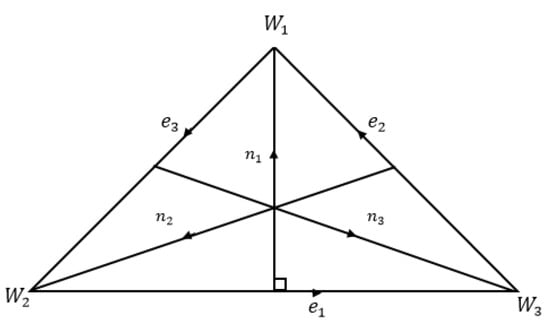
Figure 5. Inward normal direction to the edges of triangle.

The normal derivatives of local scheme $T_1, T_2,T_3$ are defined by

$$\begin{array}{cc}\hfill D_{n1}{T}_1=& (4t_{120}-2t_{021}-3t_{030})v^2+(4t_{102}-2t_{012}-3t_{003})w^2\hfill \\ & +2(3t_{111}^1-2t_{021}-2t_{012})vw+v{t}_{030}+w{t}_{003}\hfill \\ \hfill D_{n2}{T}_2=& (4t_{120}-2t_{021}-3t_{030})u^2+(4t_{102}-2t_{012}-3t_{003})w^2\hfill \\ & +2(3t_{111}^2-2t_{021}-2t_{012})vw+v{t}_{030}+w{t}_{003}\hfill \\ \hfill D_{n3}{T}_3=& (4t_{120}-2t_{021}-3t_{030})u^2+(4t_{102}-2t_{012}-3t_{003})v^2\hfill \\ & +2(3t_{111}^2-2t_{021}-2t_{012})uv+u{t}_{030}+v{t}_{003}\hfill \end{array}\}.$$

(8)

The boundary ordinates are given as follows [2]:

$$t_{210}=t_{300}+\frac{1}{4}\left[\left(x_2-x_1\right)T_x\left(W_1\right)+\left(y_2-y_1\right)T_y\left(W_1\right)\right],$$

$$t_{201}=t_{300}+\frac{1}{4}\left[\left(x_1-x_3\right)T_x\left(W_1\right)+\left(y_1-y_3\right)T_y\left(W_1\right)\right],$$

$$t_{012}=t_{030}+\frac{1}{4}\left[\left(x_3-x_2\right)T_x\left(W_2\right)+\left(y_3-y_2\right)T_y\left(W_2\right)\right],$$

$$t_{120}=t_{030}+\frac{1}{4}\left[\left(x_2-x_1\right)T_x\left(W_2\right)+\left(y_2-y_1\right)T_y\left(W_2\right)\right],$$

$$t_{102}=t_{003}+\frac{1}{4}\left[\left(x_1-x_3\right)T_x\left(W_3\right)+\left(y_1-y_3\right)T_y\left(W_3\right)\right],$$

and

$$t_{012}=t_{003}+\frac{1}{4}\left[\left(x_3-x_2\right)T_x\left(W_3\right)+\left(y_3-y_2\right)T_y\left(W_3\right)\right].$$

where the first partial derivatives $T_x\left(W_1\right), T_y\left(W_1\right)$ are estimated by using Goodman et al. [18] method. The inner ordinates i.e., $t_{111}^i, i=1,2,3$ are obtained by using two different methods i.e., Goodman and Said [8] and Foley and Opitz [19]. The following paragraphs describes both methods.

The inner ordinates by using Goodman and Said [8] method are given as follows [2]:

$$a_{111}^1=\frac{2}{3}\left(a_{120}+a_{102}\right)+\frac{1}{3}\left(a_{021}+a_{012}\right)-\frac{1}{2}\left(a_{030}+a_{003}\right),$$

$$a_{111}^2=\frac{2}{3}\left(a_{210}+a_{012}\right)+\frac{1}{3}\left(a_{201}+a_{102}\right)-\frac{1}{2}\left(a_{300}+a_{003}\right),$$

and

$$a_{111}^3=\frac{2}{3}\left(a_{201}+a_{021}\right)+\frac{1}{3}\left(a_{210}+a_{120}\right)-\frac{1}{2}\left(a_{300}+a_{030}\right).$$

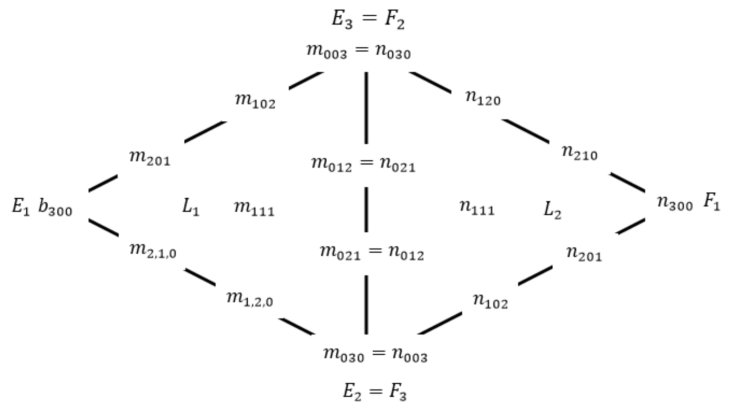
Foley and Opitz’s [19] method is as follows. Assume two adjacent triangles,$L_1, L_2$ as shown in Figure 6 with vertices $E_i$ and $F_i$ with $e_1$ as a common edge (see Figure 6).

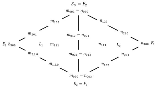
Figure 6. Two adjacent cubic triangular patches for Foley and Opitz [19].

The following equations must be satisfied to produce $C^1$ continuity along the common edge.

$$n_{201}=r^2{m}_{210}+2st{m}_{021}+2rs{m}_{120}+s^2{m}_{030}+2rt{m}_{111}^1+t^2{m}_{012} ,$$

(9)

$$n_{210}=r^2{m}_{201}+2st{m}_{012}+2rt{m}_{102}+s^2{m}_{021}+2rs{m}_{111}^1+t^2{m}_{003} ,$$

(10)

$$m_{201}=u^2{n}_{201}+2vw{n}_{012}+2uw{n}_{102}+v^2{n}_{021}+2uv{n}_{111}^1+w^2{n}_{003} ,$$

(11)

$$m_{201}=u^2{n}_{210}+2vw{n}_{021}+2uv{n}_{120}+v^2{n}_{030}+2uw{n}_{111}^1+w^2{n}_{012 },$$

(12)

where $F_1=r{E}_1+s{E}_2+t{E}_3$ and $E_1=u{F}_1+v{F}_2+w{F}_3.$ Equations $\left(9\right)$ and $\left(10\right)$ will be added together to obtain the inner ordinate $m_{111}^1$. Then, solve for $m_{111}^1$:

$$\begin{array}{c}{m}_{111}^1=\frac{1}{2u\left(v+w\right)}\left(n_{201}+n_{210}\right)-u^2\left(m_{210}+m_{201}\right)-v^2\left(m_{030}+m_{021}\right)\hfill \\ -w^2\left(m_{012}+m_{003}\right)-2vw\left(m_{021}+m_{012}\right)-uv{m}_{120}-2uw{m}_{102}.\hfill \end{array}$$

(13)

This calculation is similar to obtain the inner ordinate $n_{111}^1$. Adding the Equations $\left(11\right)$ and $\left(12\right)$ and the value of $n_{111}^1$ is given as:

$$\begin{array}{c}{n}_{111}^1=\frac{1}{2r\left(s+t\right)}\left(m_{201}+m_{210}\right)-r^2\left(n_{210}+n_{201}\right)-s^2\left(n_{030}+n_{021}\right)-t^2\left(n_{012}+n_{003}\right)\hfill \\ -2st\left(n_{021}+n_{012}\right)-rs{n}_{120}-2rt{n}_{102}.\hfill \end{array}$$

(14)

To produce the final interpolant, two methods of convex combination mentioned in Equation (6) will be used. The final scheme of scattered data interpolation using cubic Timmer triangular patch can be expressed as Theorem 3.

Theorem 3:

The final interpolating surface T on each triangle can be expressed as:

$$T\left(u,v,w\right)={\alpha }_1{T}_1\left(u,v,w\right)+{\alpha }_2{T}_2\left(u,v,w\right)+{\alpha }_3{T}_3\left(u,v,w\right)$$

where

$${\alpha }_1=\frac{vw}{vw+uv+uw},{\alpha }_2=\frac{uw}{vw+uv+uw},{\alpha }_3=\frac{uv}{vw+uv+uw}$$

Equivalently

$$T\left(u,v,w\right)={\displaystyle \sum }_{\begin{array}{c}i+j+k=3,\\ i\ne 1, j\ne 1, k\ne 1,\end{array}}{t}_{ijk}T\left(u,v,w\right)+6uvw\left({\alpha }_1{t}_{111}^1+{\beta }_2{t}_{111}^2+{\gamma }_3{t}_{111}^3\right).$$

(15)

Another version of convex combination scheme is presented in Goodman and Said [8] and is given as follows:

$${\alpha }_1=\frac{v^2{w}^2}{v^2{w}^2+u^2{v}^2+u^2{w}^2},{\alpha }_2=\frac{u^2{w}^2}{v^2{w}^2+u^2{v}^2+u^2{w}^2}, {\alpha }_3=\frac{u^2{v}^2}{v^2{w}^2+u^2{v}^2+u^2{w}^2}.$$

(16)

For the purpose of numerical comparison later, we denoted convex combination used in Equation (6) as Choice 1; meanwhile, Goodman and Said [8] is Choice 2.

Theorem 4:

The rational corrected interpolant defined by (8) is in the form quantic numerator and quadratic denominator.

Proof. 

From Equation (8), the resulting interpolant is degree 7 i.e., degree five in numerator and degree two in denominator. □

The following Algorithm 1 can be used to construct surface form scattered date.

Algorithm 1. Construction scattered data interpolation

Input: Data points

Triangulate the domain by using Delaunay triangulation. Specify the derivatives at the data points using [18] then assign Timmer ordinates values for each triangular patch. Generate the triangular patches of the surfaces by using cubic Timmer triangular patches. Calculate CPU time (in seconds), RMSE, maximum error and R2. Output: Surface reconstruction    Steps 1–4 are repeated for different test function.

4. Results and Discussions

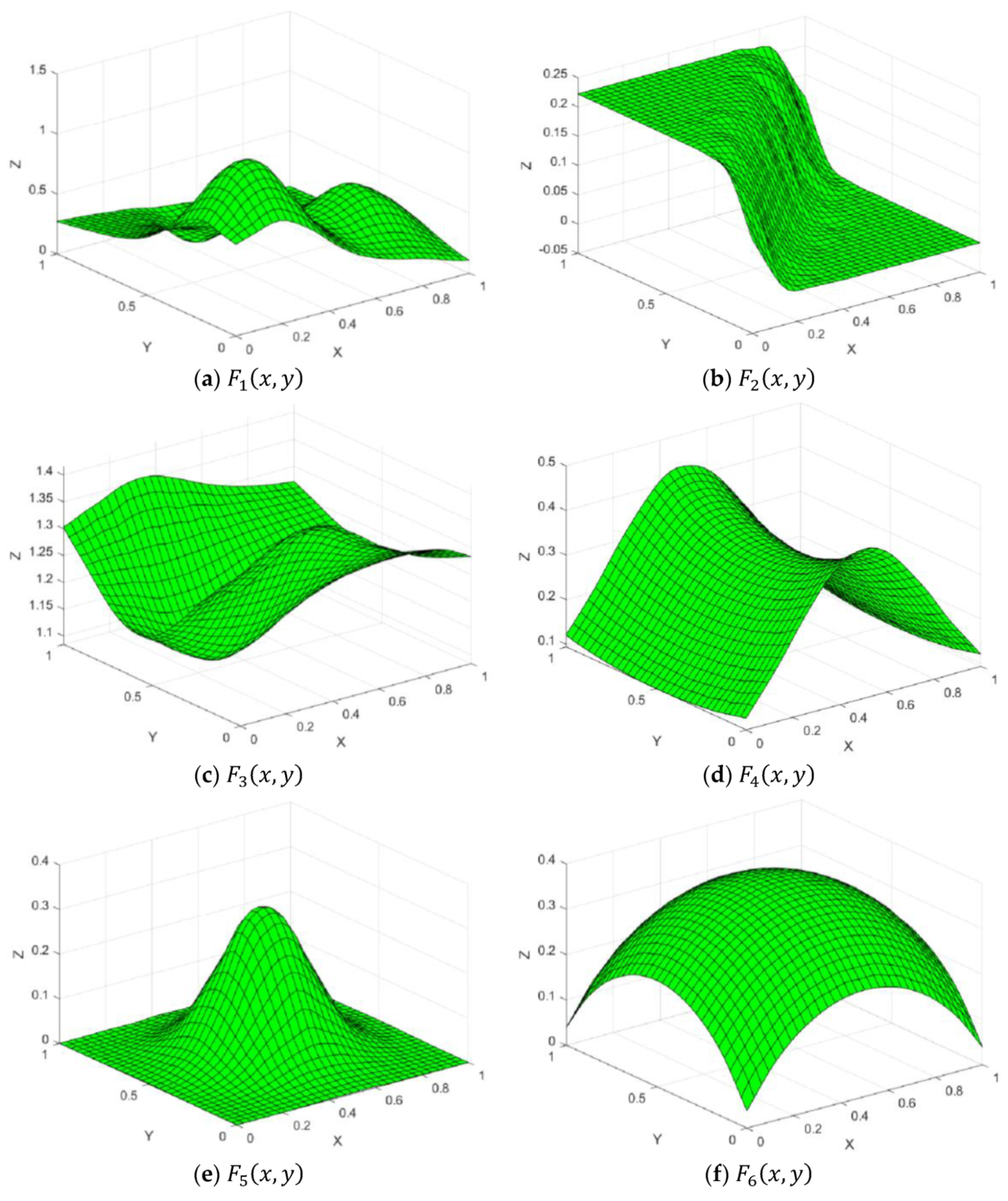
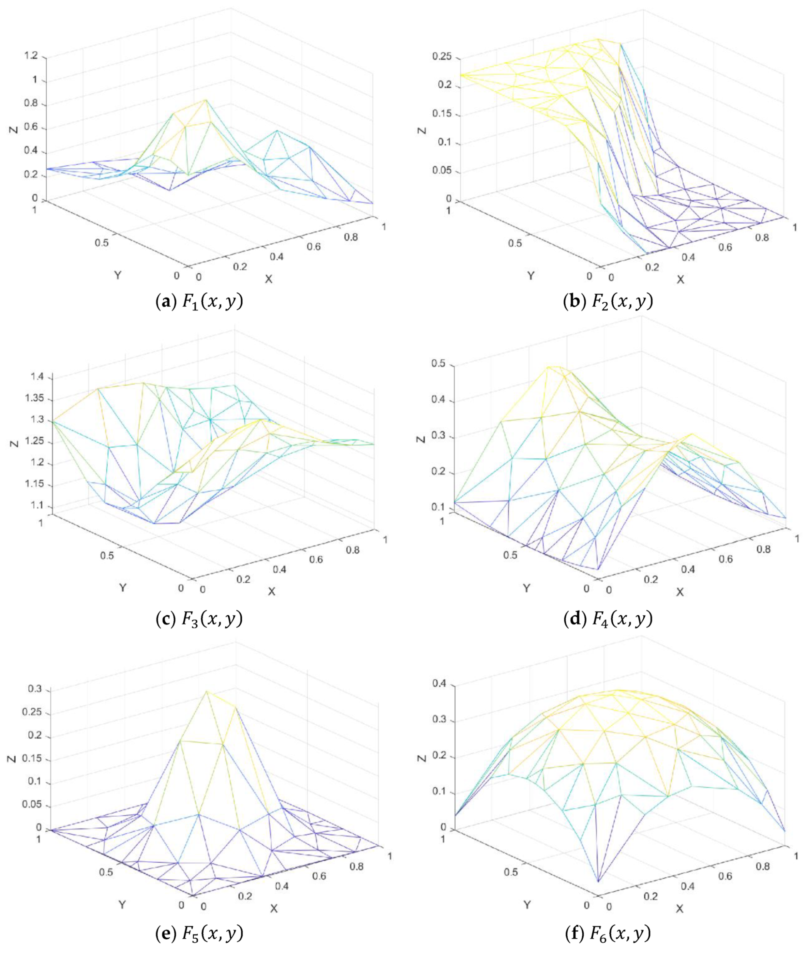
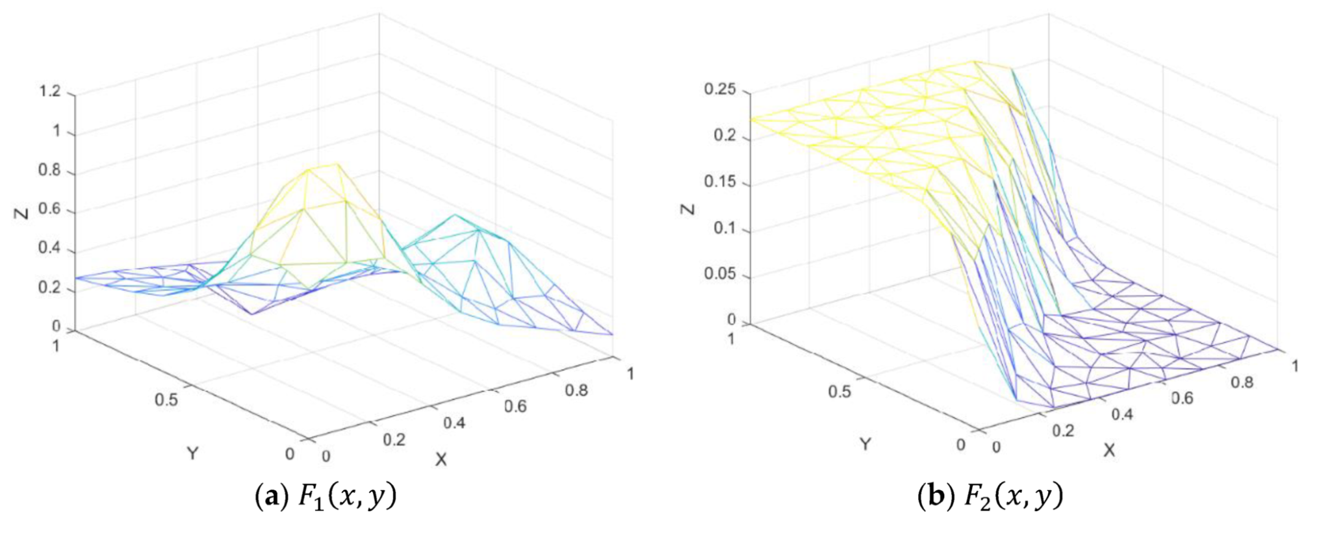
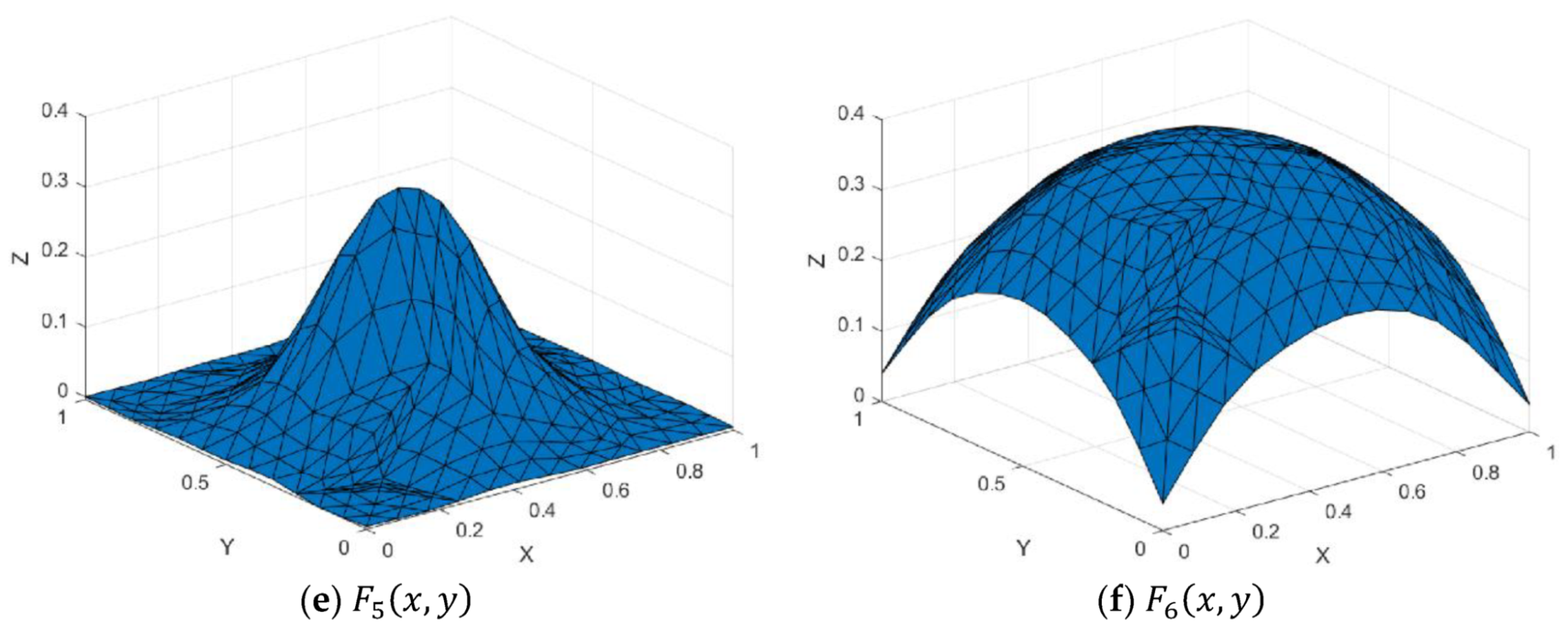
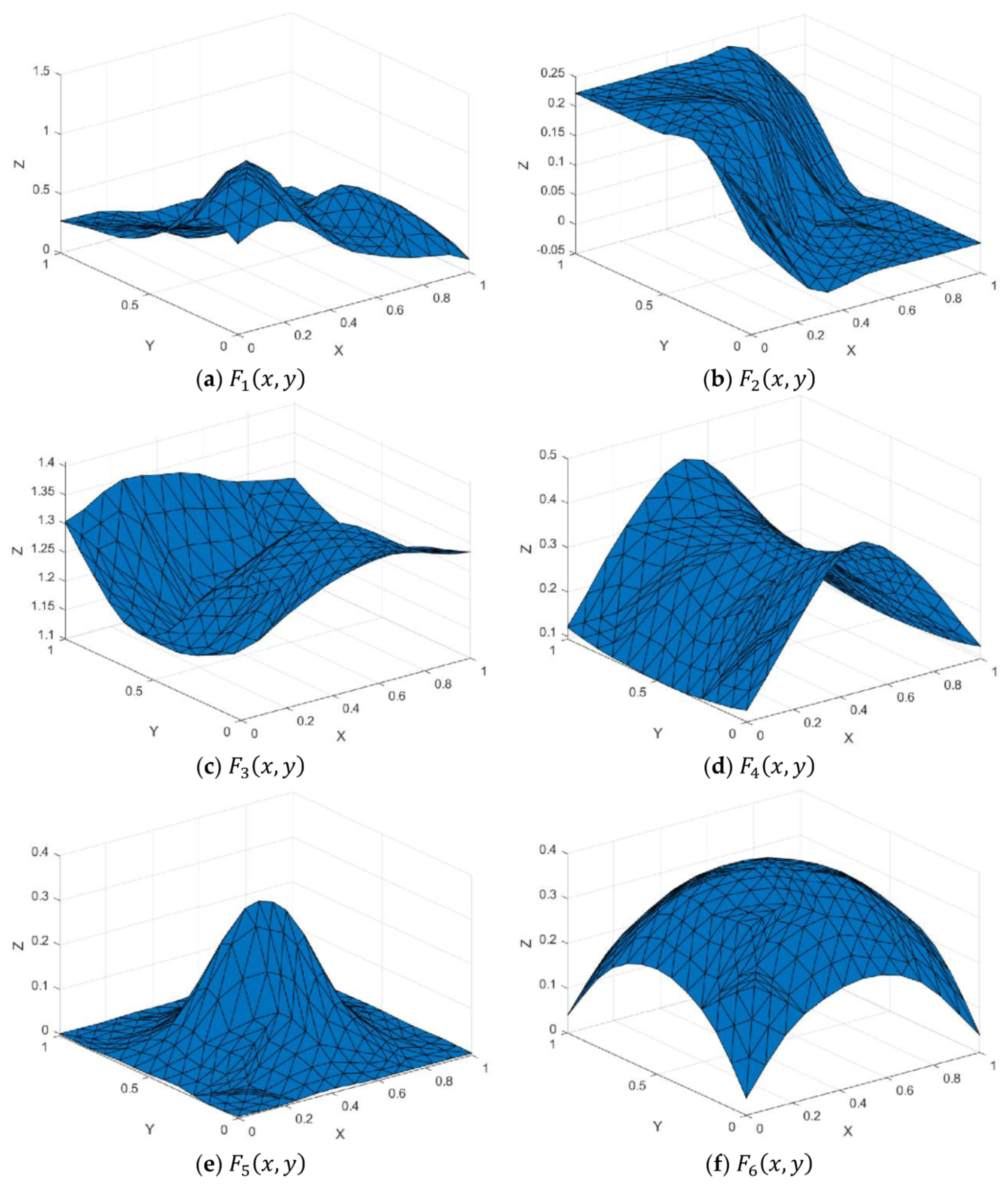
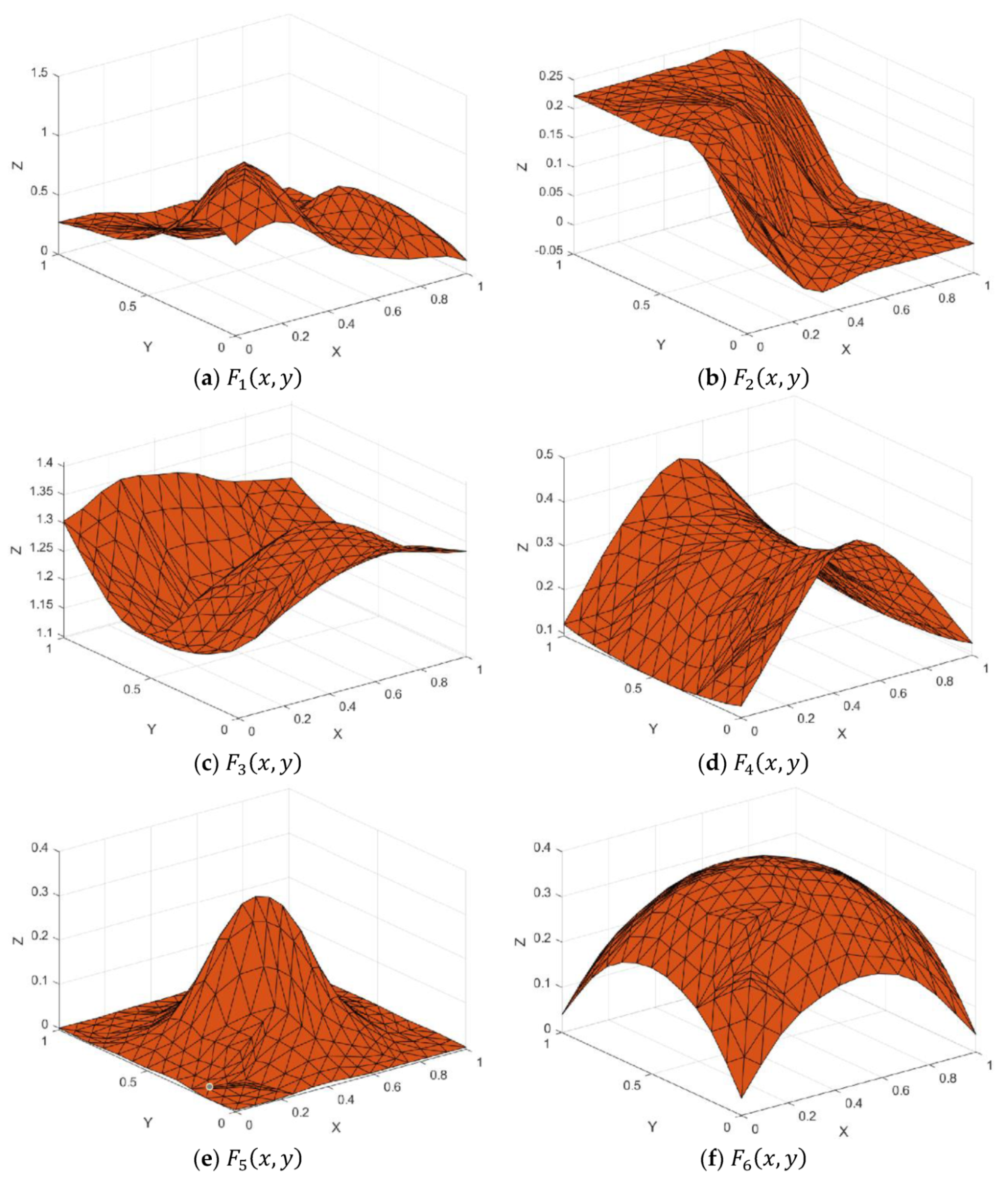
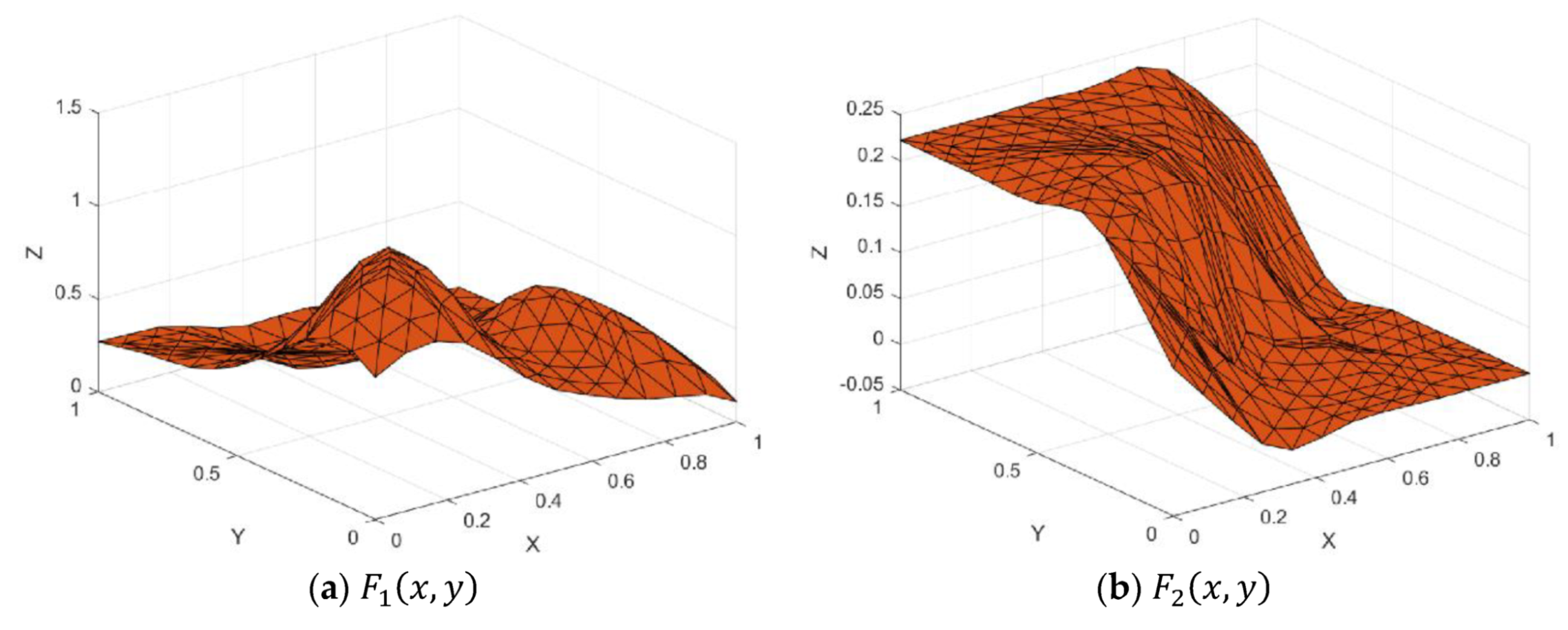
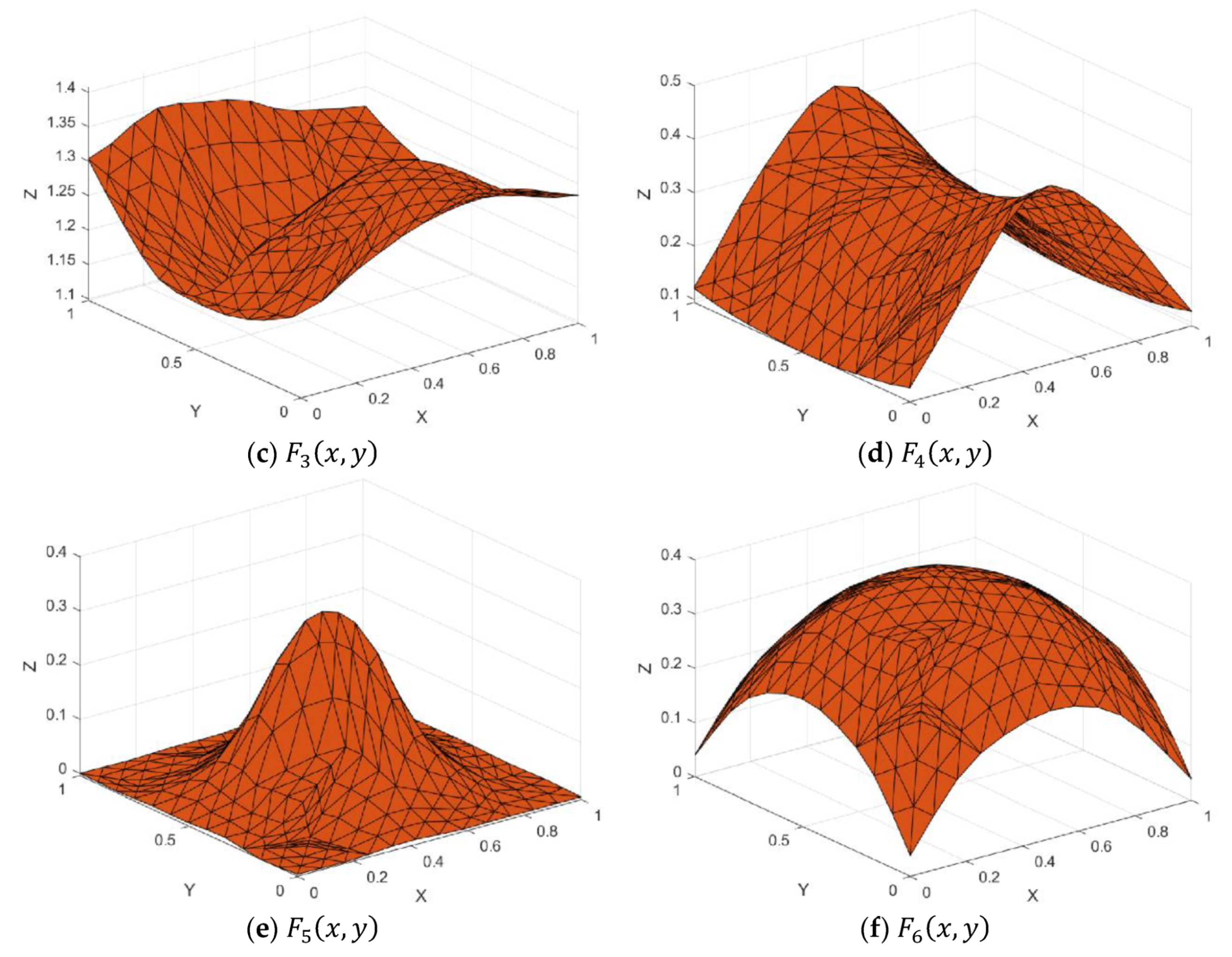
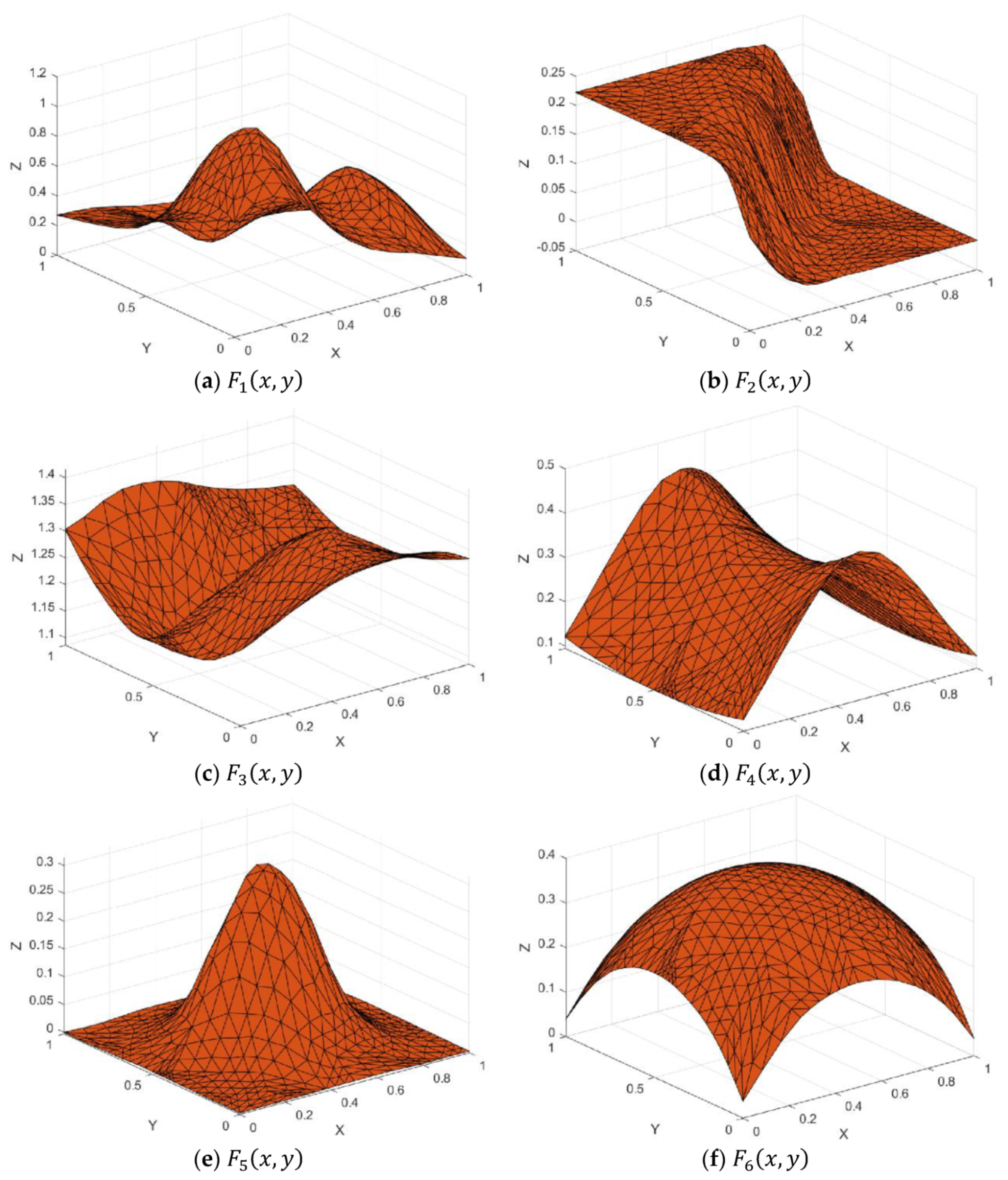
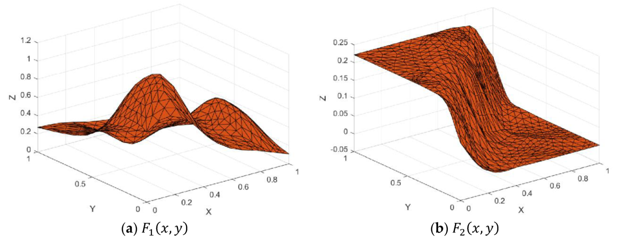
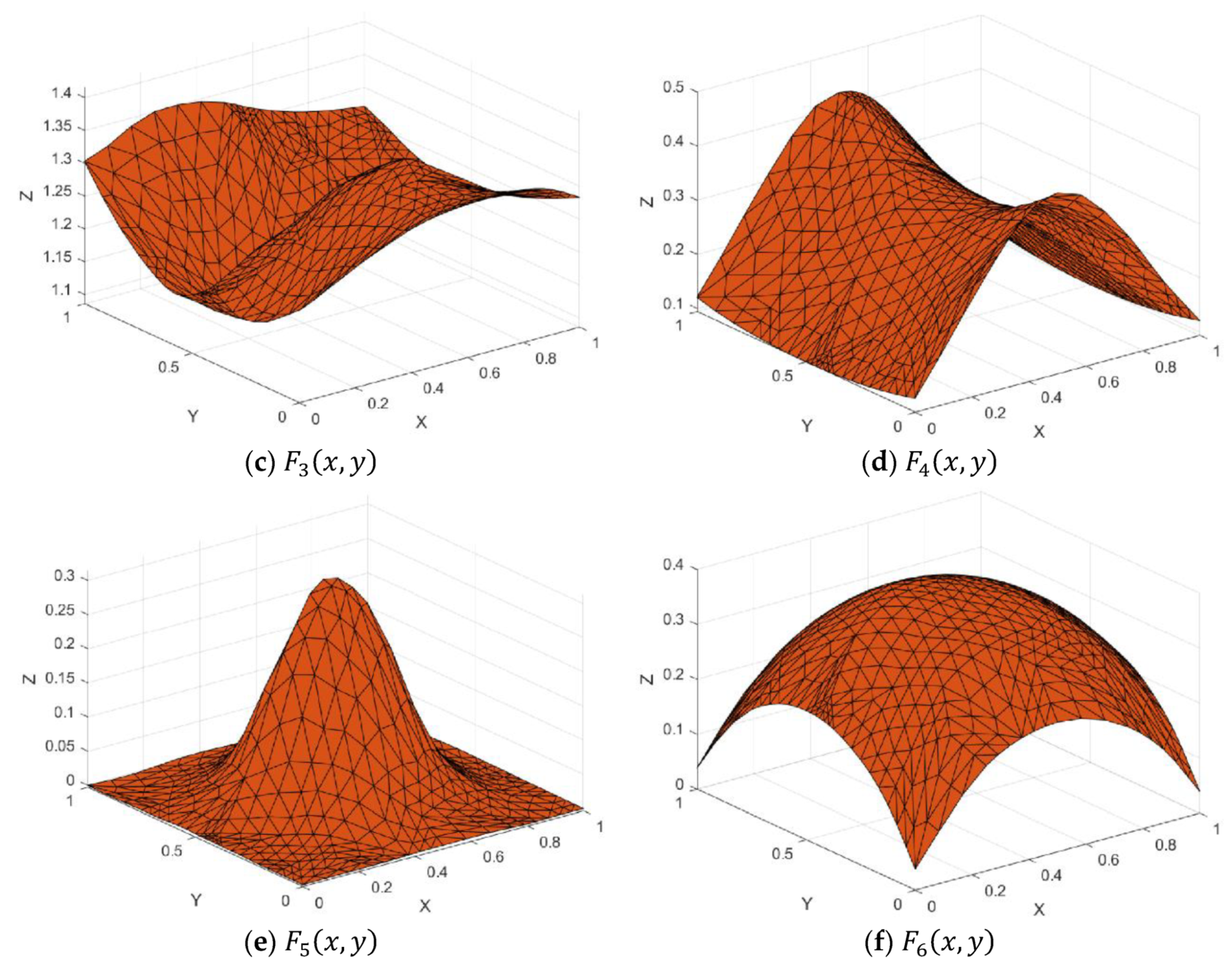
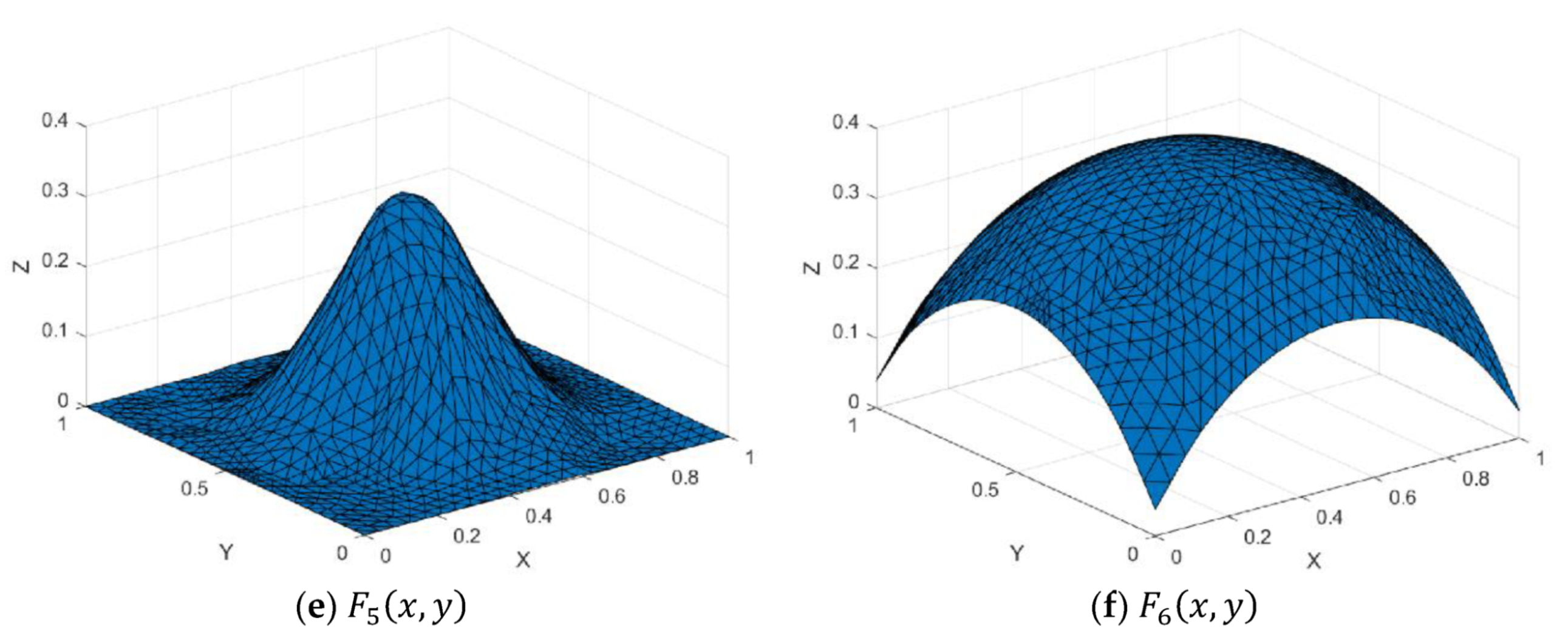
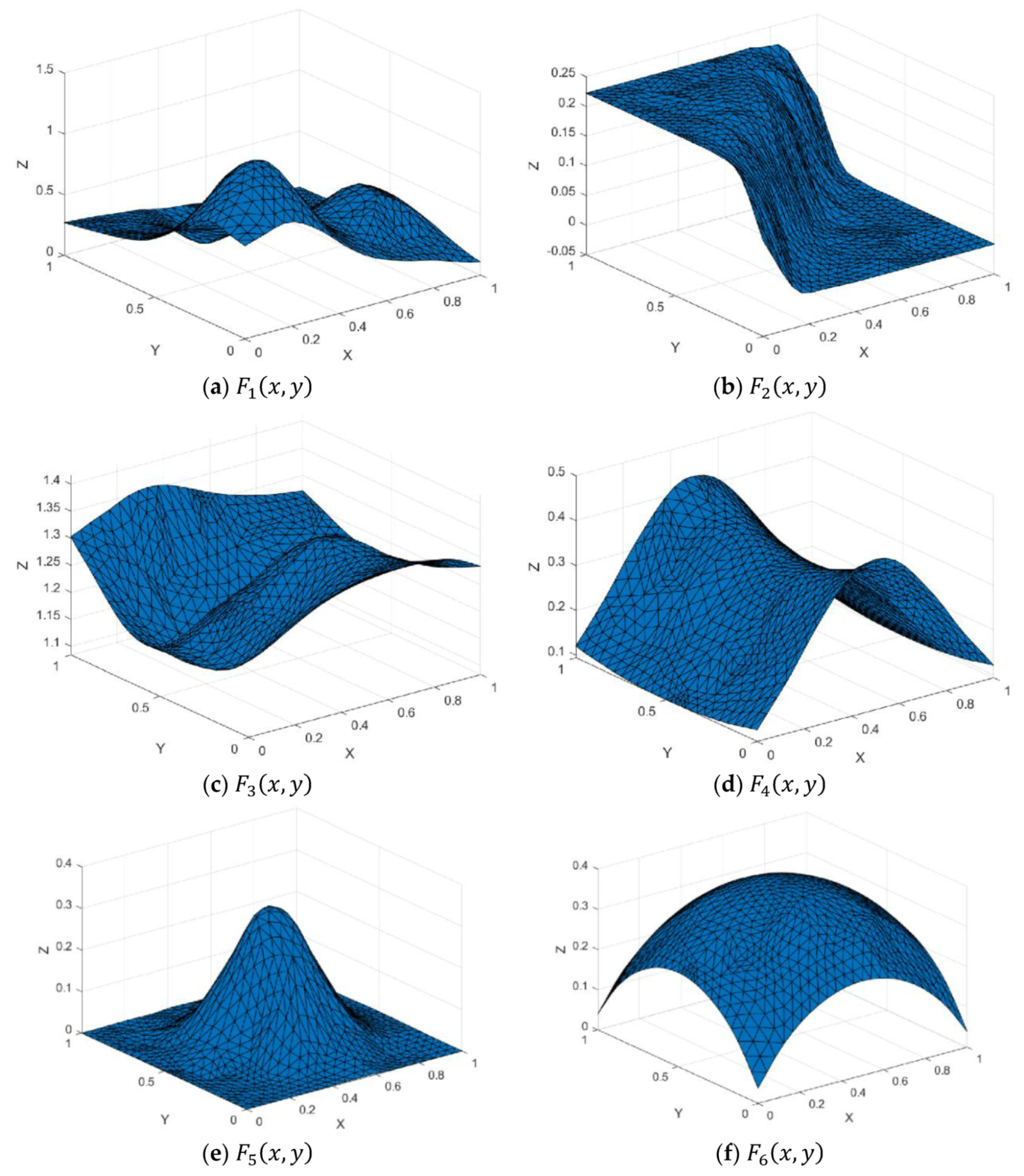
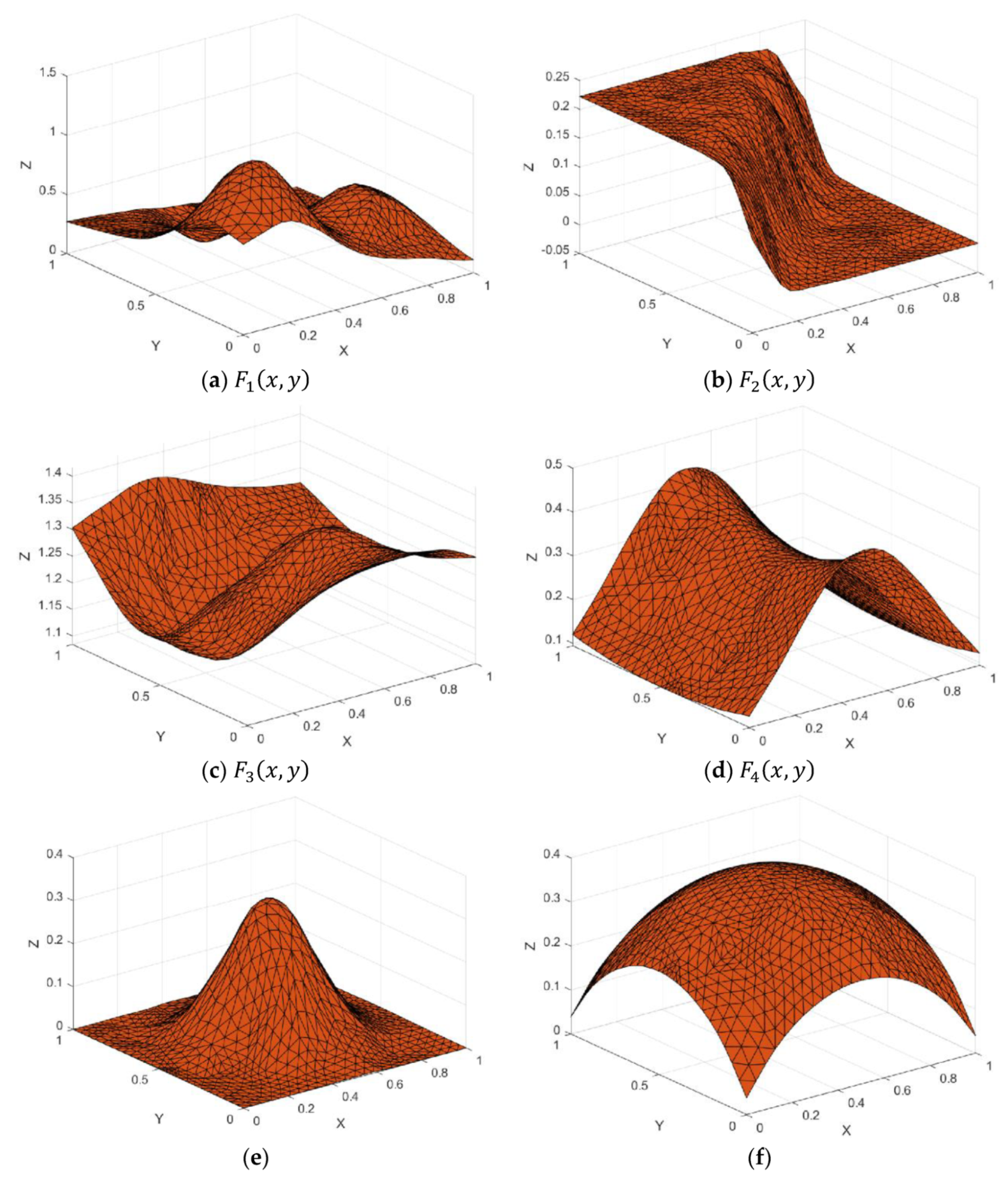
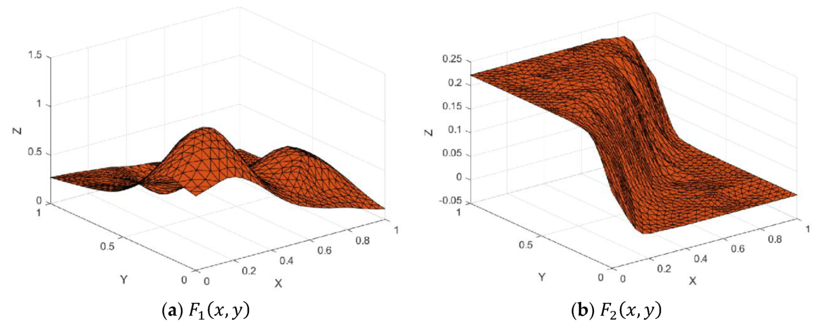
To test the capability of the proposed scattered data interpolation scheme, we use six well-known test functions $F_1\left(x,y\right),F_2\left(x,y\right),F_3\left(x,y\right),F_4\left(x,y\right),F_5\left(x,y\right)$, and $F_6\left(x,y\right)$ as shown in Figure 7 [20]. All numerical simulation and graphical visualization are done by using MATLAB R2019a version on Intel^® Core i5–6200U 2.3GHz with Turbo Boost up to 2.8GHz.

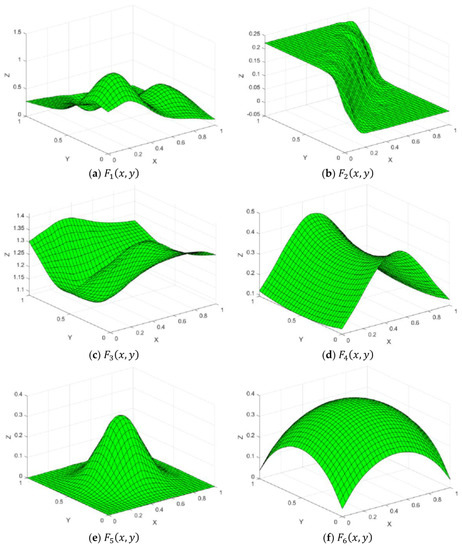
Figure 7. Test functions.

• Franke’s exponential function

$$F_1\left(x,y\right)=0.75e^{-\left(\frac{{(9x-2)}^2+{(9y-2)}^2}{4}\right)}+0.75e^{-\left(\frac{{(9x+1)}^2}{49}+\frac{9y+1}{10}\right)}+0.50e^{-\left(\frac{{(9x-7)}^2+{(9y-3)}^2}{4}\right)}-0.20e^{-\left({(9x-4)}^2+{\left(9y-7\right)}^2\right)};$$

2.

Cliff function

$$F_2\left(x,y\right)=\frac{\tanh \left(9y-9x\right)+1}{9};$$

3.

Saddle function

$$F_3\left(x,y\right)=\frac{1.25+\cos \left(4.5y\right)}{6+6{\left(3x-1\right)}^2};$$

4.

Gentle function

$$F_4\left(x,y\right)=\frac{exp\left(-\left(\frac{81}{16}\right)\left({\left(x-0.5\right)}^2+{\left(y-0.5\right)}^2\right)\right)}{3};$$

5.

Steep function

$$F_5\left(x,y\right)=\frac{exp\left(-\left(\frac{81}{4}\right)\left({\left(x-0.5\right)}^2+{\left(y-0.5\right)}^2\right)\right)}{3};$$

6.

Sphere function

$$F_6\left(x,y\right)=\frac{1}{9}\sqrt{64-81\left({\left(x-0.5\right)}^2+{\left(y-0.5\right)}^2\right)}-0.5.$$

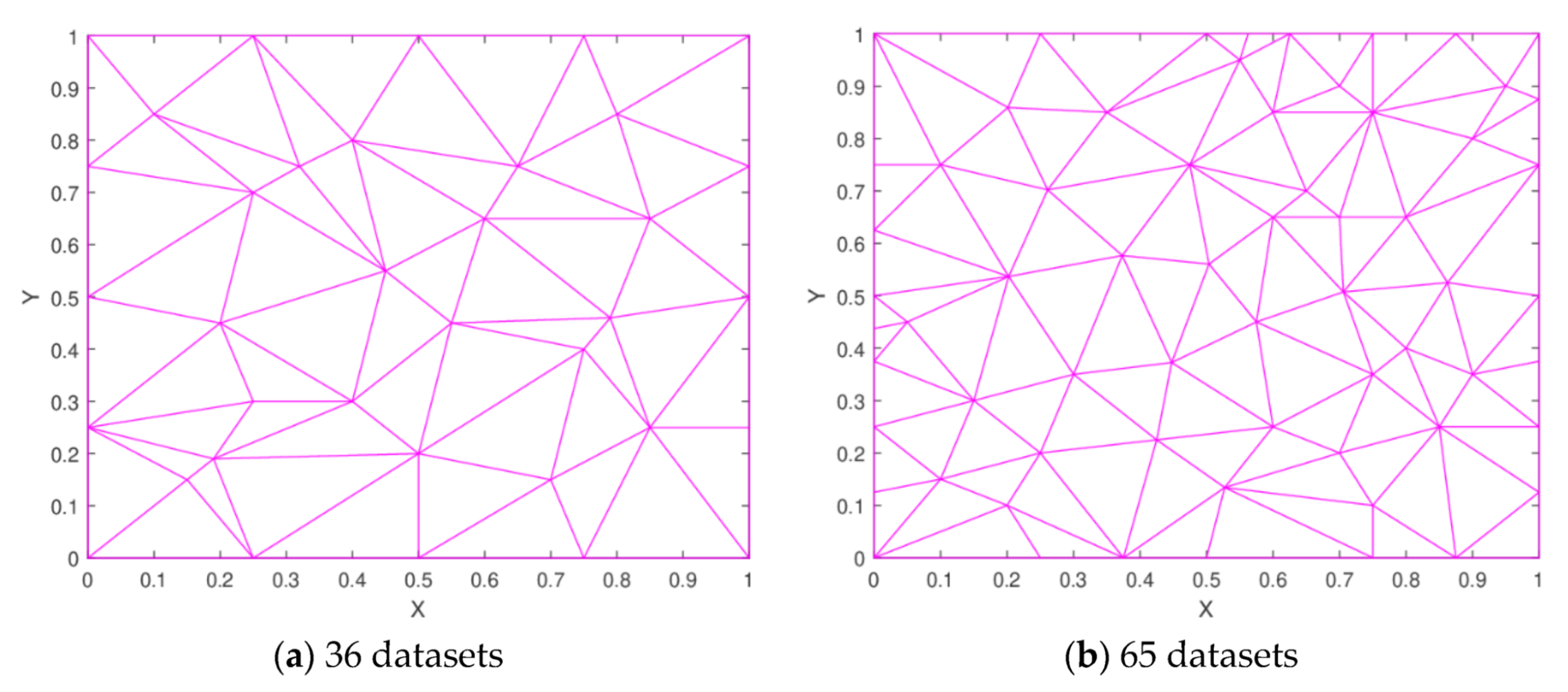
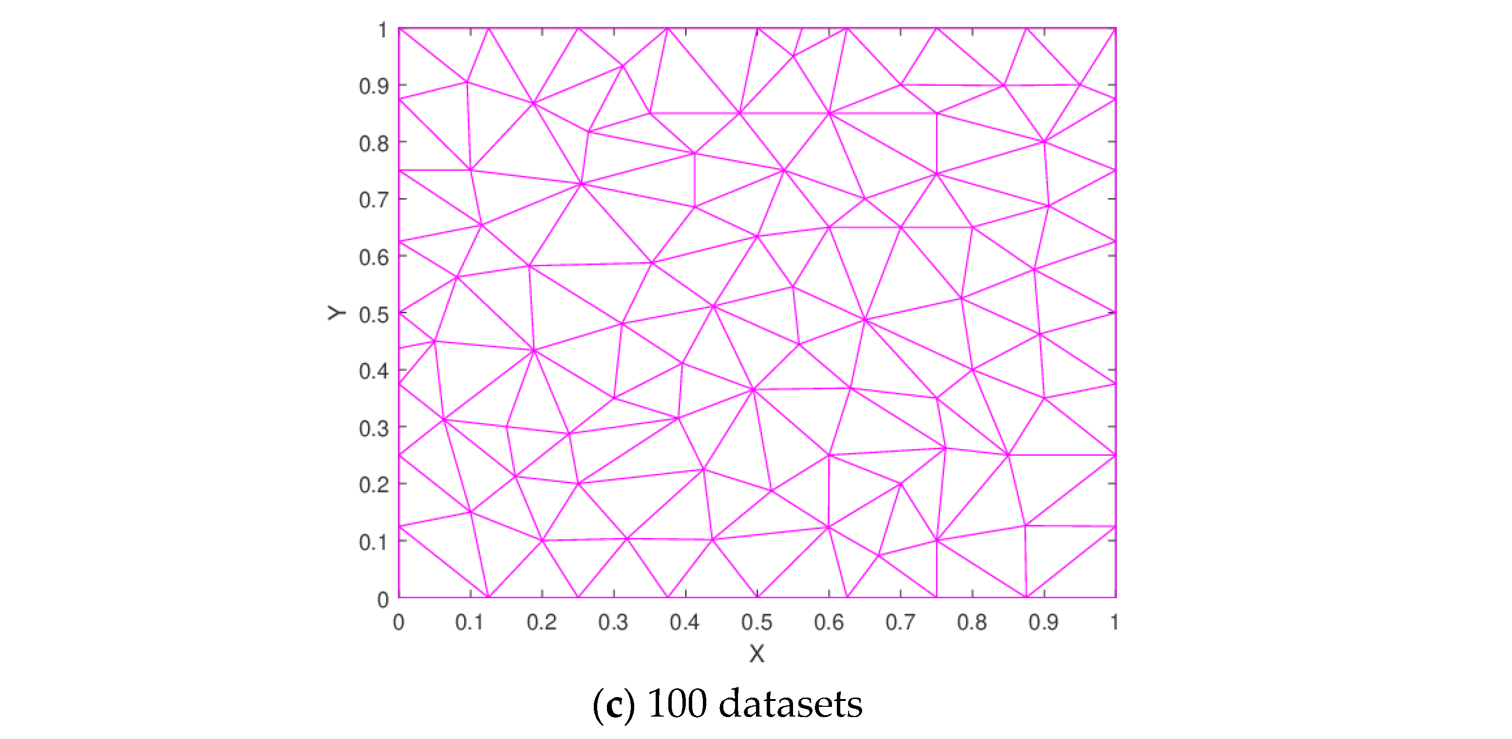
We use three datasets i.e., 36, 65, and 100 number of points, as shown in Table 2, Table 3 and Table 4.

Table 2. Thirty-six datasets.

X	Y	${\mathit{F}}_1\left(\mathit{x},\mathit{y}\right)$	${\mathit{F}}_2\left(\mathit{x},\mathit{y}\right)$	${\mathit{F}}_3\left(\mathit{x},\mathit{y}\right)$	${\mathit{F}}_4\left(\mathit{x},\mathit{y}\right)$	${\mathit{F}}_5\left(\mathit{x},\mathit{y}\right)$	${\mathit{F}}_6\left(\mathit{x},\mathit{y}\right)$
0.0000	0.0000	0.7664	0.1111	1.3333	0.1207	1.34E-05	0.0386
0.5000	0.0000	0.4349	2.74E-05	1.3833	0.4280	0.0021	0.2349
1.0000	0.0000	0.1076	3.38E-09	1.2833	0.1207	1.34E-05	0.0386
0.1500	0.1500	1.1370	0.1111	1.3382	0.2027	0.0023	0.2383
0.7000	0.1500	0.4304	1.11E-05	1.3020	0.3077	0.0124	0.2922
0.5000	0.2000	0.5345	0.0010	1.3128	0.3647	0.0539	0.3367
0.2500	0.3000	1.0726	0.1580	1.2423	0.2528	0.0418	0.3292
0.4000	0.3000	0.7134	0.0315	1.2421	0.3298	0.1211	0.3603
0.7500	0.4000	0.5903	0.0004	1.2139	0.2454	0.0768	0.3471
0.8500	0.2500	0.5088	4.53E-06	1.2607	0.1908	0.0079	0.2779
0.5500	0.4500	0.3823	0.0315	1.1613	0.3300	0.3012	0.3861
0.0000	0.5000	0.4818	0.2222	1.1747	0.0940	0.0021	0.2349
0.2000	0.4500	0.6458	0.2198	1.1412	0.2119	0.0512	0.3352
0.4500	0.5500	0.2946	0.1907	1.1037	0.3300	0.3012	0.3861
0.6000	0.6500	0.1920	0.1580	1.1552	0.3241	0.1726	0.3704
0.2500	0.7000	0.2930	0.2222	1.1240	0.2528	0.0418	0.3292
0.4000	0.8000	0.0515	0.2221	1.1887	0.3467	0.0440	0.3307
0.6500	0.7500	0.1372	0.1907	1.1961	0.3166	0.0596	0.3397
0.8000	0.8500	0.0823	0.1580	1.2431	0.2389	0.0045	0.2600
0.8500	0.6500	0.1412	0.0059	1.2043	0.1834	0.0177	0.3032
1.0000	0.5000	0.1610	2.74E-05	1.2199	0.0940	0.0021	0.2349
1.0000	1.0000	0.0359	0.1111	1.2712	0.1207	1.34E-05	0.0386
0.5000	1.0000	0.1460	0.2222	1.3346	0.4280	0.0021	0.2349
0.1000	0.8500	0.2935	0.2222	1.2363	0.1676	0.0011	0.2125
0.0000	1.0000	0.2703	0.2222	1.3029	0.1207	1.34E-05	0.0386
0.2500	0.0000	0.8189	0.0024	1.4069	0.3119	0.0006	0.1911
0.7500	0.0000	0.2521	3.05E-07	1.3150	0.3119	0.0006	0.1911
0.2500	1.0000	0.2222	0.2222	1.3496	0.3119	0.0006	0.1911
0.0000	0.2500	0.8026	0.2198	1.2683	0.1001	0.0006	0.1911
0.7500	1.0000	0.0810	0.2198	1.2913	0.3119	0.0006	0.1911
0.0000	0.7500	0.3395	0.2222	1.1987	0.1001	0.0006	0.1911
1.0000	0.2500	0.2302	3.05E-07	1.2573	0.1001	0.0006	0.1911
1.0000	0.7500	0.0504	0.0024	1.2295	0.1001	0.0006	0.1911
0.1900	0.1900	1.2118	0.1111	1.3229	0.2256	0.0068	0.2733
0.3200	0.7500	0.2029	0.2221	1.1477	0.3012	0.0488	0.3338
0.7900	0.4600	0.4777	0.0006	1.2041	0.2181	0.0588	0.3393

Table 3. Sixty-five datasets.

X	Y	${\mathit{F}}_1\left(\mathit{x},\mathit{y}\right)$	${\mathit{F}}_2\left(\mathit{x},\mathit{y}\right)$	${\mathit{F}}_3\left(\mathit{x},\mathit{y}\right)$	${\mathit{F}}_4\left(\mathit{x},\mathit{y}\right)$	${\mathit{F}}_5\left(\mathit{x},\mathit{y}\right)$	${\mathit{F}}_6\left(\mathit{x},\mathit{y}\right)$
0.0500	0.4500	0.5775	0.0024	1.1767	0.3119	0.0052	0.2649
0.0000	0.5000	0.4818	3.05E-07	1.1747	0.3119	0.0021	0.2349
0.0000	1.0000	0.2703	3.05E-07	1.3029	0.1001	1.34E-05	0.0386
0.0000	0.0000	0.7664	0.0024	1.3333	0.1001	1.34E-05	0.0386
0.1000	0.1500	1.0495	0.2198	1.3271	0.3119	0.0011	0.2125
0.1000	0.7500	0.3229	0.2222	1.1812	0.3119	0.0037	0.2534
0.1500	0.3000	1.0600	0.2222	1.2437	0.1001	0.0124	0.2922
0.2000	0.1000	1.0774	0.2198	1.3732	0.1001	0.0021	0.2349
0.2500	0.2000	1.1892	0.2010	1.3239	0.2100	0.0152	0.2985
0.3000	0.3500	0.8562	2.89E-06	1.1982	0.0955	0.0940	0.3530
0.3500	0.8500	0.1588	0.0212	1.2297	0.1082	0.0177	0.3032
0.5000	0.0000	0.4349	0.2220	1.3833	0.3955	0.0021	0.2349
0.5000	1.0000	0.1460	0.2220	1.3346	0.0955	0.0021	0.2349
0.5500	0.9500	0.1329	0.2010	1.2975	0.1082	0.0052	0.2649
0.2500	0.0000	0.8189	0.0004	1.4069	0.3373	0.0006	0.1911
0.7500	0.0000	0.2521	0.1580	1.3150	0.3241	0.0006	0.1911
1.0000	0.2500	0.2302	0.2198	1.2573	0.3582	0.0006	0.1911
1.0000	0.7500	0.0504	0.1580	1.2295	0.3096	0.0006	0.1911
0.7500	1.0000	0.0810	2.74E-05	1.2913	0.2979	0.0006	0.1911
0.2500	1.0000	0.2222	0.0642	1.3496	0.2784	0.0006	0.1911
0.0000	0.7500	0.3395	0.2163	1.1987	0.3195	0.0006	0.1911
0.0000	0.2500	0.8026	1.84E-06	1.2683	0.2851	0.0006	0.1911
0.8750	1.0000	0.0553	0.0002	1.2791	0.2484	0.0001	0.1321
1.0000	0.3750	0.2405	0.1907	1.2354	0.2746	0.0015	0.2242
1.0000	0.8750	0.0406	0.0002	1.2504	0.2135	0.0001	0.1321
0.6250	1.0000	0.1124	0.0140	1.3099	0.2162	0.0015	0.2242
0.0000	0.3750	0.6464	4.53E-06	1.2134	0.1908	0.0015	0.2242
0.0000	0.1250	0.8220	1.11E-05	1.3151	0.1517	0.0001	0.1321
0.6000	0.2500	0.5050	0.0315	1.2723	0.1623	0.0768	0.3471
0.6000	0.6500	0.1920	0.0642	1.1552	0.1403	0.1726	0.3704
0.6000	0.8500	0.1196	3.38E-09	1.2376	0.1207	0.0228	0.3109
0.6500	0.7000	0.1585	2.74E-05	1.1796	0.0940	0.0940	0.3530
0.7000	0.2000	0.5070	0.1111	1.2855	0.1207	0.0240	0.3125
0.7000	0.6500	0.1854	0.2221	1.1796	0.4196	0.0940	0.3530
0.7000	0.9000	0.1021	0.2221	1.2611	0.0944	0.0058	0.2682
0.7500	0.1000	0.3475	0.0059	1.3058	0.3494	0.0037	0.2534
0.7500	0.3500	0.6368	0.0212	1.2296	0.3248	0.0596	0.3397
0.7500	0.8500	0.0948	0.2167	1.2421	0.3091	0.0079	0.2779
0.8000	0.4000	0.5729	0.0457	1.2187	0.3341	0.0440	0.3307
0.8000	0.6500	0.1608	0.2222	1.1975	0.2414	0.0342	0.3232
0.8500	0.2500	0.5088	0.2221	1.2607	0.2601	0.0079	0.2779
0.9000	0.3500	0.4588	0.2217	1.2366	0.2132	0.0083	0.2795
0.9000	0.8000	0.0654	3.21E-08	1.2336	0.1082	0.0021	0.2349
0.9500	0.9000	0.0473	3.21E-08	1.2555	0.2100	0.0002	0.1539
1.0000	0.0000	0.1076	0.2207	1.2833	0.3537	1.34E-05	0.0386
1.0000	0.5000	0.1610	0.0005	1.2199	0.1715	0.0021	0.2349
1.0000	1.0000	0.0359	0.0003	1.2712	0.3955	1.34E-05	0.0386
0.5625	1.0000	0.1292	0.0002	1.3218	0.3797	0.0019	0.2323
0.0000	0.4375	0.5564	0.0061	1.1907	0.2690	0.0019	0.2323
0.4250	0.2250	0.7025	0.1634	1.3040	0.3345	0.0643	0.3419
0.5750	0.4500	0.3940	0.2222	1.1673	0.0955	0.2828	0.3843
0.3732	0.5768	0.3115	0.1111	1.0857	0.1207	0.2136	0.3764
0.4475	0.3725	0.5128	0.1111	1.1864	0.1207	0.2268	0.3781
0.2013	0.8592	0.2658	0.1111	1.2395	0.1207	0.0040	0.2562
0.2611	0.7021	0.2857	0.1111	1.1232	0.1207	0.0459	0.3320
0.2024	0.5368	0.4564	0.1111	1.1098	0.1207	0.0540	0.3368
1.0000	0.1250	0.1552	0.1111	1.2760	0.1207	0.0001	0.1321
0.8750	0.0000	0.1796	0.1111	1.2958	0.1207	0.0001	0.1321
0.4750	0.7500	0.0247	0.1111	1.1632	0.1207	0.0928	0.3526
0.8625	0.5250	0.2938	0.1111	1.2049	0.1207	0.0230	0.3112
0.3750	0.0000	0.6331	0.1111	1.4141	0.1207	0.0015	0.2242
0.5273	0.1341	0.4668	0.1111	1.3433	0.1207	0.0218	0.3096
0.7058	0.5073	0.3878	0.1111	1.1818	0.1207	0.1412	0.3647
0.5037	0.5605	0.2694	0.1111	1.1187	0.1207	0.3094	0.3868
0.0000	0.6250	0.3892	0.1111	1.1689	0.1207	0.0015	0.2242

Table 4. One hundred datasets.

X	Y	${\mathit{F}}_1\left(\mathit{x},\mathit{y}\right)$	${\mathit{F}}_2\left(\mathit{x},\mathit{y}\right)$	${\mathit{F}}_3\left(\mathit{x},\mathit{y}\right)$	${\mathit{F}}_4\left(\mathit{x},\mathit{y}\right)$	${\mathit{F}}_5\left(\mathit{x},\mathit{y}\right)$	${\mathit{F}}_6\left(\mathit{x},\mathit{y}\right)$
0.0500	0.4500	0.5775	0.2221	1.1767	0.1199	0.0052	0.2649
0.0000	0.5000	0.4818	0.2222	1.1747	0.0940	0.0021	0.2349
0.0000	1.0000	0.2703	0.2222	1.3029	0.1207	0.0000	0.0386
0.0000	0.0000	0.7664	0.1111	1.3333	0.1207	0.0000	0.0386
0.1000	0.1500	1.0495	0.1580	1.3271	0.1676	0.0011	0.2125
0.1000	0.7500	0.3229	0.2222	1.1812	0.1578	0.0037	0.2534
0.1500	0.3000	1.0600	0.2082	1.2437	0.1866	0.0124	0.2922
0.2000	0.1000	1.0774	0.0315	1.3732	0.2480	0.0021	0.2349
0.2500	0.2000	1.1892	0.0642	1.3239	0.2658	0.0152	0.2985
0.3000	0.3500	0.8562	0.1580	1.1982	0.2784	0.0940	0.3530
0.3500	0.8500	0.1588	0.2222	1.2297	0.3362	0.0177	0.3032
0.5000	0.0000	0.4349	0.0000	1.3833	0.4280	0.0021	0.2349
0.5000	1.0000	0.1460	0.2222	1.3346	0.4280	0.0021	0.2349
0.5500	0.9500	0.1329	0.2221	1.2975	0.4030	0.0052	0.2649
0.6000	0.2500	0.5050	0.0004	1.2723	0.3373	0.0768	0.3471
0.6000	0.6500	0.1920	0.1580	1.1552	0.3241	0.1726	0.3704
0.6000	0.8500	0.1196	0.2198	1.2376	0.3582	0.0228	0.3109
0.6500	0.7000	0.1585	0.1580	1.1796	0.3096	0.0940	0.3530
0.7000	0.2000	0.5070	0.0000	1.2855	0.2979	0.0240	0.3125
0.7000	0.6500	0.1854	0.0642	1.1796	0.2784	0.0940	0.3530
0.7000	0.9000	0.1021	0.2163	1.2611	0.3195	0.0058	0.2682
0.7500	0.1000	0.3475	0.0000	1.3058	0.2851	0.0037	0.2534
0.7500	0.3500	0.6368	0.0002	1.2296	0.2484	0.0596	0.3397
0.7500	0.8500	0.0948	0.1907	1.2421	0.2746	0.0079	0.2779
0.8000	0.4000	0.5729	0.0002	1.2187	0.2135	0.0440	0.3307
0.8000	0.6500	0.1608	0.0140	1.1975	0.2162	0.0342	0.3232
0.8500	0.2500	0.5088	0.0000	1.2607	0.1908	0.0079	0.2779
0.9000	0.3500	0.4588	0.0000	1.2366	0.1517	0.0083	0.2795
0.9000	0.8000	0.0654	0.0315	1.2336	0.1623	0.0021	0.2349
0.9500	0.9000	0.0473	0.0642	1.2555	0.1403	0.0002	0.1539
1.0000	0.0000	0.1076	0.0000	1.2833	0.1207	0.0000	0.0386
0.0000	0.6250	0.3892	0.2222	1.1689	0.0955	0.0015	0.2242
0.6250	0.0000	0.3203	0.0000	1.3444	0.3955	0.0015	0.2242
0.8750	0.0000	0.1796	0.0000	1.2958	0.2100	0.0001	0.1321
0.0000	0.8750	0.3026	0.2222	1.2511	0.1082	0.0001	0.1321
0.4386	0.5114	0.3383	0.1750	1.1093	0.3271	0.3080	0.3867
0.1816	0.5822	0.4015	0.2221	1.1119	0.2009	0.0373	0.3258
0.4250	0.2250	0.7025	0.0059	1.3040	0.3494	0.0643	0.3419
0.4750	0.8500	0.0579	0.2220	1.2328	0.3756	0.0275	0.3167
0.4125	0.6855	0.1477	0.2206	1.1163	0.3319	0.1422	0.3649
0.5993	0.1237	0.4060	0.0000	1.3299	0.3653	0.0155	0.2992
1.0000	0.1250	0.1552	0.0000	1.2760	0.1082	0.0001	0.1321
0.1250	1.0000	0.2516	0.2222	1.3261	0.2100	0.0001	0.1321
0.1875	0.8675	0.2679	0.2222	1.2461	0.2327	0.0030	0.2466
0.1250	0.0000	0.8467	0.0212	1.3699	0.2100	0.0001	0.1321
0.7500	0.7438	0.1181	0.1049	1.2083	0.2578	0.0282	0.3174
0.2545	0.7263	0.2787	0.2222	1.1378	0.2586	0.0349	0.3238
0.8938	0.4625	0.3559	0.0001	1.2152	0.1522	0.0140	0.2960
1.0000	0.6250	0.0831	0.0003	1.2176	0.0955	0.0015	0.2242
0.7844	0.5250	0.3500	0.0021	1.1939	0.2215	0.0640	0.3418
0.9063	0.6875	0.0943	0.0042	1.2145	0.1497	0.0058	0.2680
0.8859	0.5758	0.1981	0.0008	1.2056	0.1577	0.0145	0.2972
0.5375	0.7500	0.0842	0.2175	1.1755	0.3523	0.0914	0.3522
0.1886	0.4341	0.6915	0.2196	1.1520	0.2049	0.0428	0.3299
0.3112	0.4806	0.4971	0.2122	1.1082	0.2784	0.1607	0.3684
0.4943	0.3652	0.4735	0.0198	1.1972	0.3394	0.2306	0.3786
0.3528	0.5875	0.3139	0.2190	1.0840	0.3010	0.1841	0.3722
0.3750	1.0000	0.1842	0.2222	1.3542	0.3955	0.0015	0.2242
0.3125	0.9333	0.2109	0.2222	1.3034	0.3366	0.0037	0.2531
0.8441	0.8987	0.0676	0.1617	1.2570	0.2146	0.0012	0.2161
0.3954	0.4113	0.5277	0.1269	1.1525	0.3179	0.2278	0.3782
0.3899	0.3149	0.7178	0.0457	1.2291	0.3244	0.1303	0.3624
1.0000	0.5000	0.1610	0.0000	1.2199	0.0940	0.0021	0.2349
1.0000	1.0000	0.0359	0.1111	1.2712	0.1207	0.0000	0.0386
0.2500	0.0000	0.8189	0.0024	1.4069	0.3119	0.0006	0.1911
0.7500	0.0000	0.2521	0.0000	1.3150	0.3119	0.0006	0.1911
1.0000	0.2500	0.2302	0.0000	1.2573	0.1001	0.0006	0.1911
1.0000	0.7500	0.0504	0.0024	1.2295	0.1001	0.0006	0.1911
0.7500	1.0000	0.0810	0.2198	1.2913	0.3119	0.0006	0.1911
0.2500	1.0000	0.2222	0.2222	1.3496	0.3119	0.0006	0.1911
0.0000	0.7500	0.3395	0.2222	1.1987	0.1001	0.0006	0.1911
0.0000	0.2500	0.8026	0.2198	1.2683	0.1001	0.0006	0.1911
0.8750	1.0000	0.0553	0.2010	1.2791	0.2100	0.0001	0.1321
1.0000	0.3750	0.2405	0.0000	1.2354	0.0955	0.0015	0.2242
1.0000	0.8750	0.0406	0.0212	1.2504	0.1082	0.0001	0.1321
0.6250	1.0000	0.1124	0.2220	1.3099	0.3955	0.0015	0.2242
0.0000	0.3750	0.6464	0.2220	1.2134	0.0955	0.0015	0.2242
0.0000	0.1250	0.8220	0.2010	1.3151	0.1082	0.0001	0.1321
0.5625	1.0000	0.1292	0.2221	1.3218	0.4196	0.0019	0.2323
0.0000	0.4375	0.5564	0.2221	1.1907	0.0944	0.0019	0.2323
0.6500	0.4875	0.3944	0.0113	1.1735	0.2975	0.2107	0.3761
0.0811	0.5625	0.4329	0.2222	1.1446	0.1376	0.0088	0.2815
0.1154	0.6538	0.3598	0.2222	1.1420	0.1614	0.0103	0.2865
0.3750	0.0000	0.6331	0.0003	1.4141	0.3955	0.0015	0.2242
0.3181	0.1035	0.9263	0.0046	1.3910	0.3299	0.0071	0.2745
0.5197	0.1873	0.5032	0.0006	1.3174	0.3669	0.0457	0.3318
0.4371	0.1016	0.6122	0.0005	1.3796	0.3829	0.0124	0.2921
0.1625	0.2125	1.1918	0.1580	1.3042	0.2034	0.0062	0.2704
0.2375	0.2875	1.1146	0.1580	1.2528	0.2460	0.0331	0.3222
0.0625	0.3125	0.8667	0.2198	1.2383	0.1310	0.0034	0.2507
0.7625	0.2625	0.6033	0.0000	1.2596	0.2488	0.0264	0.3154
0.6298	0.3677	0.5269	0.0020	1.2125	0.3115	0.1663	0.3694
0.5495	0.5455	0.2811	0.1071	1.1349	0.3299	0.3042	0.3863
0.4999	0.6340	0.1996	0.2040	1.1219	0.3394	0.2317	0.3787
0.5581	0.4443	0.3918	0.0254	1.1656	0.3287	0.2924	0.3852
0.4125	0.7796	0.0310	0.2219	1.1740	0.3467	0.0586	0.3392

5. Numerical Results

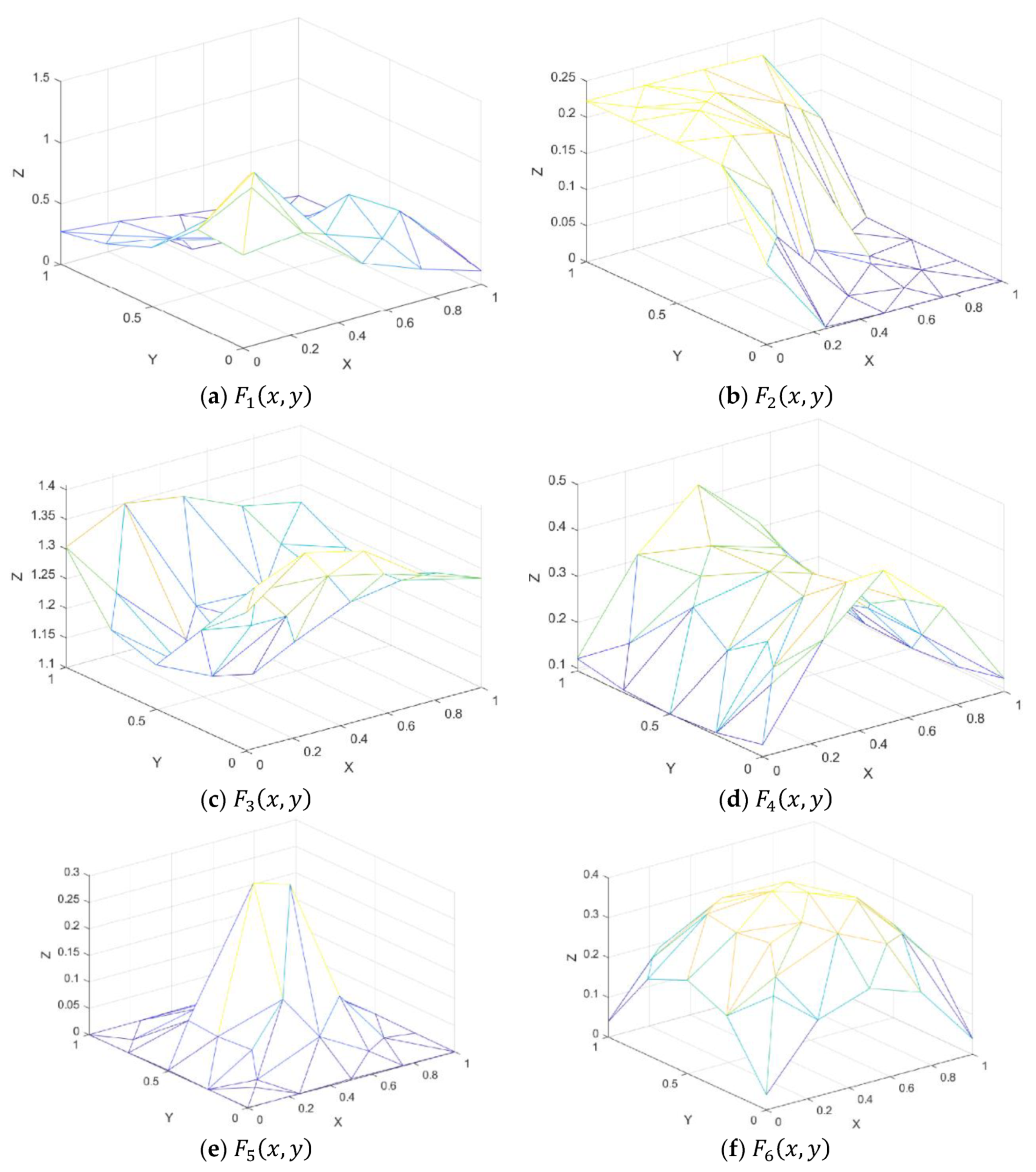
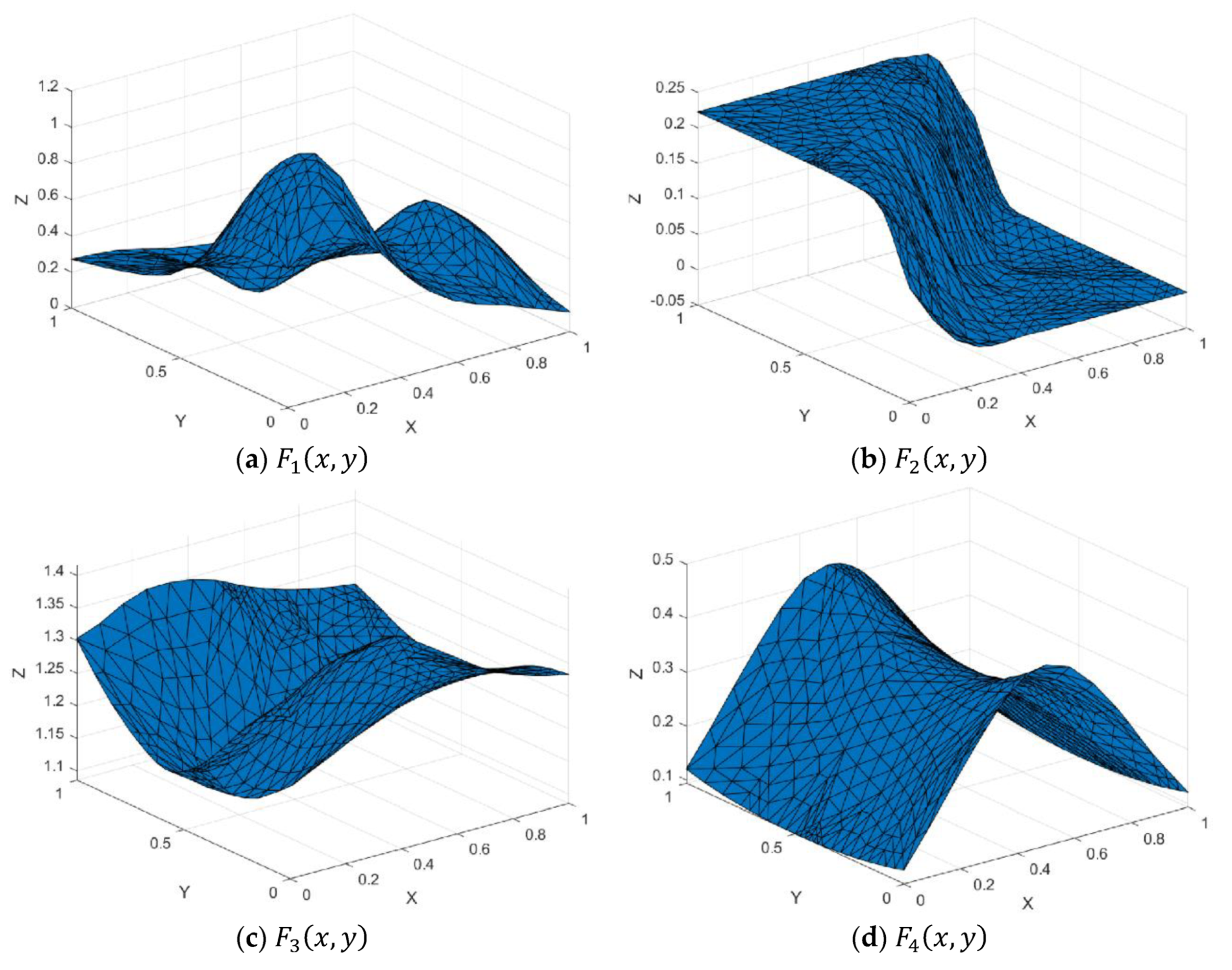
Delaunay triangulation for all datasets are shown in Figure 8. Meanwhile, Figure 9, Figure 10 and Figure 11 show the 3D linear interpolant for the scattered datasets, respectively. The surface interpolation by using cubic Timmer triangular patches with selected schemes are shown in Figure 12, Figure 13, Figure 14, Figure 15, Figure 16, Figure 17, Figure 18, Figure 19, Figure 20, Figure 21, Figure 22 and Figure 23.

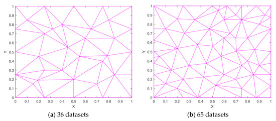
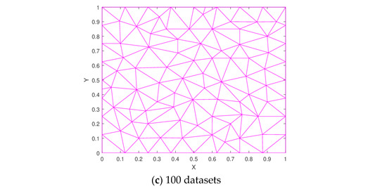
Figure 8. Delaunay triangulation.

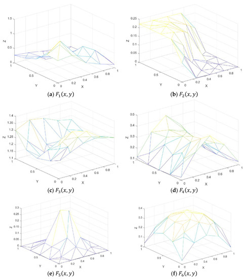
Figure 9. 3D linear interpolant for 36 datasets.

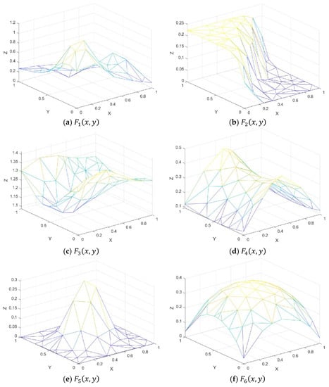
Figure 10. 3D linear interpolant for 65 datasets.

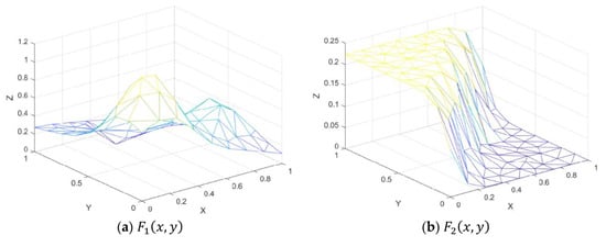
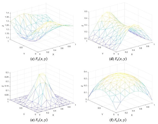
Figure 11. 3D linear interpolant for 100 datasets.

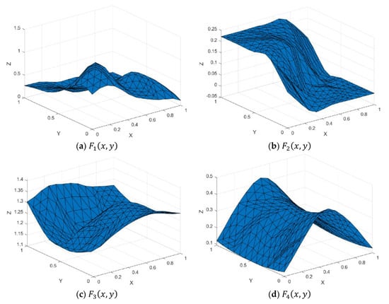
Figure 12. Surface interpolation using Goodman and Said method and Choice 1 for 36 datasets.

Figure 13. Surface interpolation using Goodman and Said method and Choice 2 for 36 datasets.

Figure 14. Surface interpolation using Foley and Opitz method and Choice 1 for 36 datasets.

Figure 15. Surface interpolation using Foley and Opitz method and Choice 2 for 36 datasets.

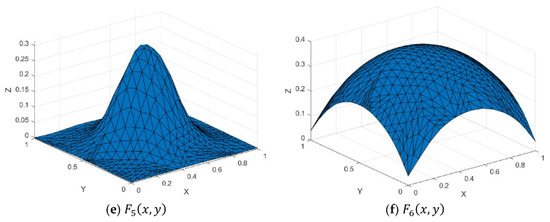
Figure 16. Surface interpolation using Goodman and Said method and Choice 1 for 65 datasets.

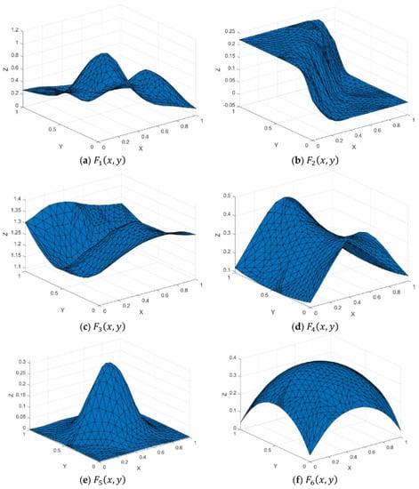
Figure 17. Surface interpolation using Goodman and Said method and Choice 2 for 65 datasets.

Figure 18. Surface interpolation using Foley and Opitz method and Choice 1 for 65 datasets.

Figure 19. Surface interpolation using Foley and Opitz method and Choice 2 for 65 datasets.

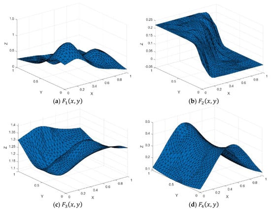
Figure 20. Surface interpolation using Goodman and Said method and Choice 1 for 100 datasets.

Figure 21. Surface interpolation using Goodman and Said method and Choice 2 for 100 datasets.

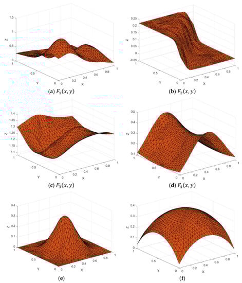
Figure 22. Surface interpolation using Foley and Opitz method and Choice 1 for 100 datasets.

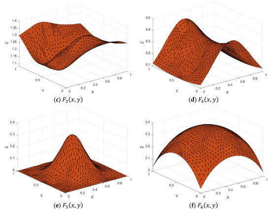
Figure 23. Surface interpolation using Foley and Opitz method and Choice 2 for 100 datasets.

Based on Figure 12, Figure 13, Figure 14, Figure 15, Figure 16, Figure 17, Figure 18, Figure 19, Figure 20, Figure 21, Figure 22 and Figure 23, all schemes are capable of producing a smooth $C^1$ surface. The 36, 65, and 100 datasets consist of 54, 100, and 164 triangular patches with $C^1$ continuity for each edge, respectively. Visually, the proposed scheme produces smooth surfaces for all datasets. However, in order to measure the effectiveness of the proposed scattered data interpolation scheme, we calculate root mean square error (RMSE), maximum error (Max error), coefficient of determination (R²), and central processor unit (CPU) time in seconds. For the computation time, a comparison has been made between two different methods to calculate the inner ordinates, i.e., Goodman and Said [8] and Foley and Opitz [19] methods and two distinct calculation of local scheme denoted as Choice 1 and Choice 2. The error analysis for 36, 65, and 100 data points are shown in Table 5, Table 6 and Table 7, respectively.

Table 5. Error analysis for 36 datasets.

Test Function	Error	Goodman and Said		Foley and Opitz
		Choice 1	Choice 2	Choice 1	Choice 2
${\mathit{F}}_{\mathbf{1}}\left(\mathit{x},\mathit{y}\right)$	RMSE	0.025827	0.025901	0.026097	0.026458
	R2	0.991858	0.991811	0.991687	0.991455
	Max error	0.109091	0.110443	0.109642	0.110142
	CPU time	3.666885	3.792837	3.531956	3.612421
${\mathit{F}}_{\mathbf{2}}\left(\mathit{x},\mathit{y}\right)$	RMSE	0.013091	0.013105	0.012899	0.012970
	R2	0.982658	0.982620	0.983163	0.982978
	Max error	0.049755	0.050222	0.048333	0.049466
	CPU time	3.465182	3.581924	3.238475	3.418465
${\mathit{F}}_{\mathbf{3}}\left(\mathit{x},\mathit{y}\right)$	RMSE	0.006086	0.006097	0.005834	0.005897
	R2	0.993518	0.993493	0.994043	0.993914
	Max error	0.026836	0.026923	0.026082	0.026475
	CPU time	3.381397	3.412042	3.362575	3.381239
${\mathit{F}}_{\mathbf{4}}\left(\mathit{x},\mathit{y}\right)$	RMSE	0.127280	0.127285	0.127392	0.127379
	R2	0.999012	0.998742	0.998671	0.998923
	Max error	0.335392	0.335392	0.335392	0.335392
	CPU time	3.718293	3.819244	3.634124	3.801234
${\mathit{F}}_{\mathbf{5}}\left(\mathit{x},\mathit{y}\right)$	RMSE	0.006244	0.006326	0.005952	0.006095
	R2	0.993218	0.993039	0.993837	0.993539
	Max error	0.030589	0.031475	0.027931	0.028902
	CPU time	3.931621	4.012938	3.544473	3.712645
${\mathit{F}}_{\mathbf{6}}\left(\mathit{x},\mathit{y}\right)$	RMSE	0.003587	0.003602	0.003980	0.003995
	R2	0.997647	0.997628	0.997104	0.997082
	Max error	0.015551	0.015589	0.015264	0.014997
	CPU time	3.910817	3.912341	3.722930	3.800012

Table 6. Error analysis for 65 datasets.

Test Function	Error	Goodman and Said		Foley and Opitz
		Choice 1	Choice 2	Choice 1	Choice 2
${\mathit{F}}_{\mathbf{1}}\left(\mathit{x},\mathit{y}\right)$	RMSE	0.015504	0.015586	0.015090	0.015246
	R2	0.997066	0.997034	0.997221	0.997163
	Max error	0.062431	0.063216	0.063829	0.066465
	CPU time	9.012512	9.214511	8.912451	9.109472
${\mathit{F}}_{\mathbf{2}}\left(\mathit{x},\mathit{y}\right)$	RMSE	0.005162	0.005177	0.005015	0.005016
	R2	0.997304	0.997288	0.997457	0.997454
	Max error	0.030704	0.030792	0.031553	0.031558
	CPU time	8.729935	9.497846	8.623959	8.761479
${\mathit{F}}_{\mathbf{3}}\left(\mathit{x},\mathit{y}\right)$	RMSE	0.003151	0.003163	0.003018	0.003091
	R2	0.998263	0.998249	0.998406	0.998328
	Max error	0.015383	0.015461	0.015825	0.016667
	CPU time	8.910241	8.948517	8.891025	8.901256
${\mathit{F}}_{\mathbf{4}}\left(\mathit{x},\mathit{y}\right)$	RMSE	0.127247	0.127249	0.127274	0.127264
	R2	0.998901	0.998703	0.998767	0.998513
	Max error	0.333987	0.333987	0.333987	0.333987
	CPU time	9.193316	9.201537	9.001285	9.182451
${\mathit{F}}_{\mathbf{5}}\left(\mathit{x},\mathit{y}\right)$	RMSE	0.004951	0.004980	0.004800	0.004877
	R2	0.995737	0.995686	0.995992	0.995863
	Max error	0.033110	0.033635	0.031342	0.031923
	CPU time	8.901256	8.924514	8.802561	8.856126
${\mathit{F}}_{\mathbf{6}}\left(\mathit{x},\mathit{y}\right)$	RMSE	0.001953	0.001959	0.002122	0.002146
	R2	0.999303	0.999298	0.999177	0.999158
	Max error	0.010602	0.010715	0.009957	0.009725
	CPU time	8.981256	8.992456	8.900128	8.941588

Table 7. Error analysis for 100 datasets.

Test Function	Error	Goodman and Said		Foley and Opitz
		Choice 1	Choice 2	Choice 1	Choice 2
${\mathit{F}}_{\mathbf{1}}\left(\mathit{x},\mathit{y}\right)$	RMSE	0.006834	0.006887	0.006660	0.006804
	R2	0.999430	0.999421	0.999459	0.999435
	Max error	0.034165	0.034446	0.032402	0.032503
	CPU time	19.245752	19.157941	18.989466	19.015484
${\mathit{F}}_{\mathbf{2}}\left(\mathit{x},\mathit{y}\right)$	RMSE	0.003638	0.003644	0.003525	0.003568
	R2	0.998661	0.998656	0.998742	0.998712
	Max error	0.023940	0.024076	0.024344	0.025017
	CPU time	17.772122	17.387878	17.726120	17.609815
${\mathit{F}}_{\mathbf{3}}\left(\mathit{x},\mathit{y}\right)$	RMSE	0.000997	0.001004	0.000960	0.001022
	R2	0.999826	0.999824	0.999839	0.999817
	Max error	0.004870	0.005009	0.004337	0.004622
	CPU time	17.377007	17.801830	16.248355	16.449573
${\mathit{F}}_{\mathbf{4}}\left(\mathit{x},\mathit{y}\right)$	RMSE	0.127213	0.127209	0.127199	0.127200
	R2	0.997790	0.997735	0.997851	0.997732
	Max error	0.334366	0.334387	0.333155	0.333431
	CPU time	18.517801	17.531418	17.221382	17. 582176
${\mathit{F}}_{\mathbf{5}}\left(\mathit{x},\mathit{y}\right)$	RMSE	0.002273	0.002299	0.002159	0.002221
	R2	0.999101	0.999081	0.999189	0.999142
	Max error	0.012672	0.012685	0.012559	0.012585
	CPU time	19.092384	19.181738	18.463083	19.083249
${\mathit{F}}_{\mathbf{6}}\left(\mathit{x},\mathit{y}\right)$	RMSE	0.001116	0.001153	0.000867	0.000868
	R2	0.999772	0.999757	0.999863	0.999862
	Max error	0.007914	0.007917	0.005458	0.005459
	CPU time	18.521953	19.728907	17.658403	18.307126

Based on Table 5, Table 6 and Table 7, the numerical results obtained by using the local scheme with Choice 2 gave larger error than Choice 1 while most of the Foley and Opitz [19] method gave smaller error than the Goodman and Said [8] method. In terms of CPU time (in seconds), the Goodman and Said [8] method takes more time than the Foley and Opitz [19] method. Convex scheme using Choice 2 took longer time than scheme with Choice 1. The main reason is because convex combination using Choice 2 requires more calculation than Choice 1. Furthermore, the reason the Foley and Opitz [19] method has less time is that their scheme considers two triangular patches to calculate the inner ordinates while the Goodman and Said [8] method needs to find the three inner ordinates for each triangular patch.

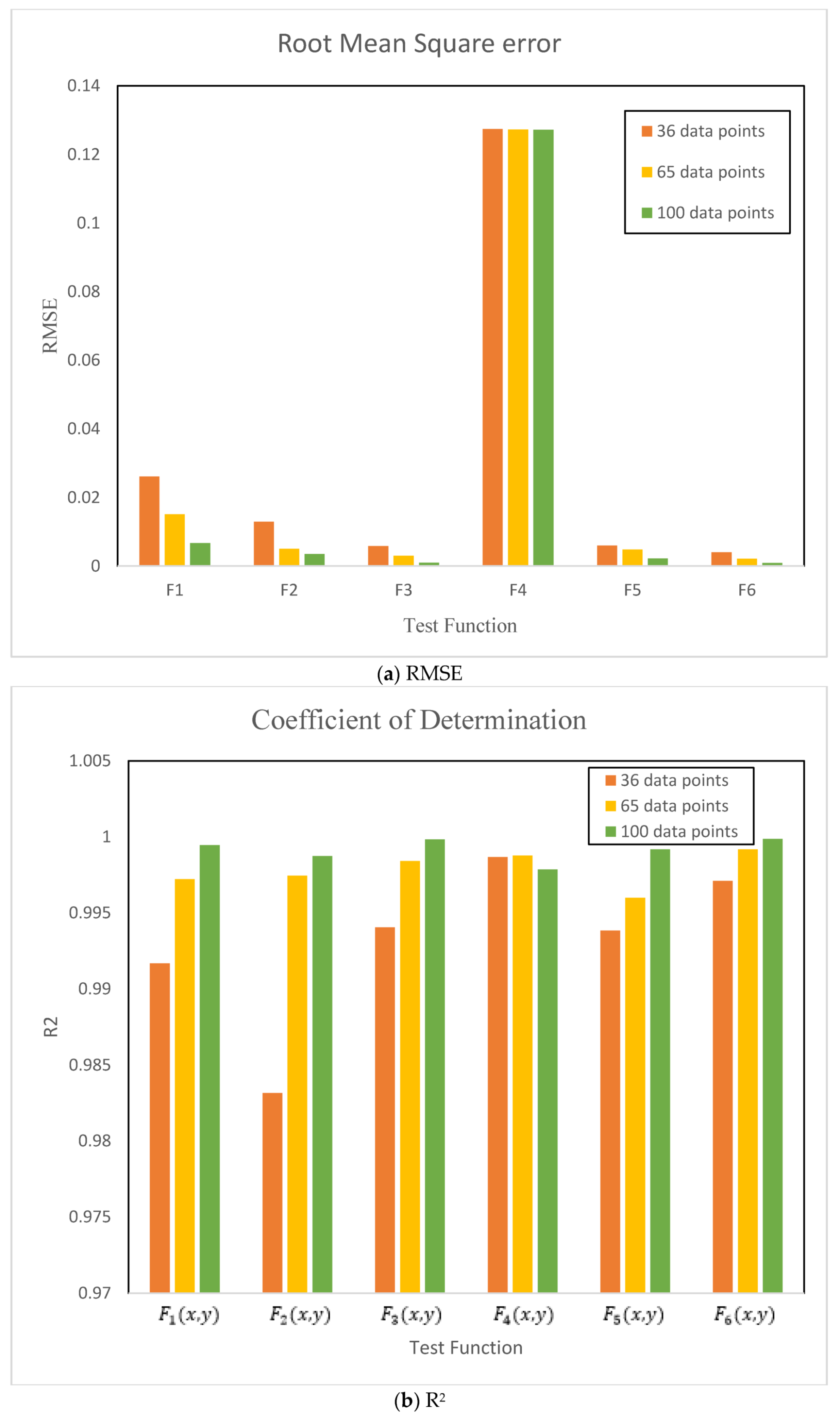
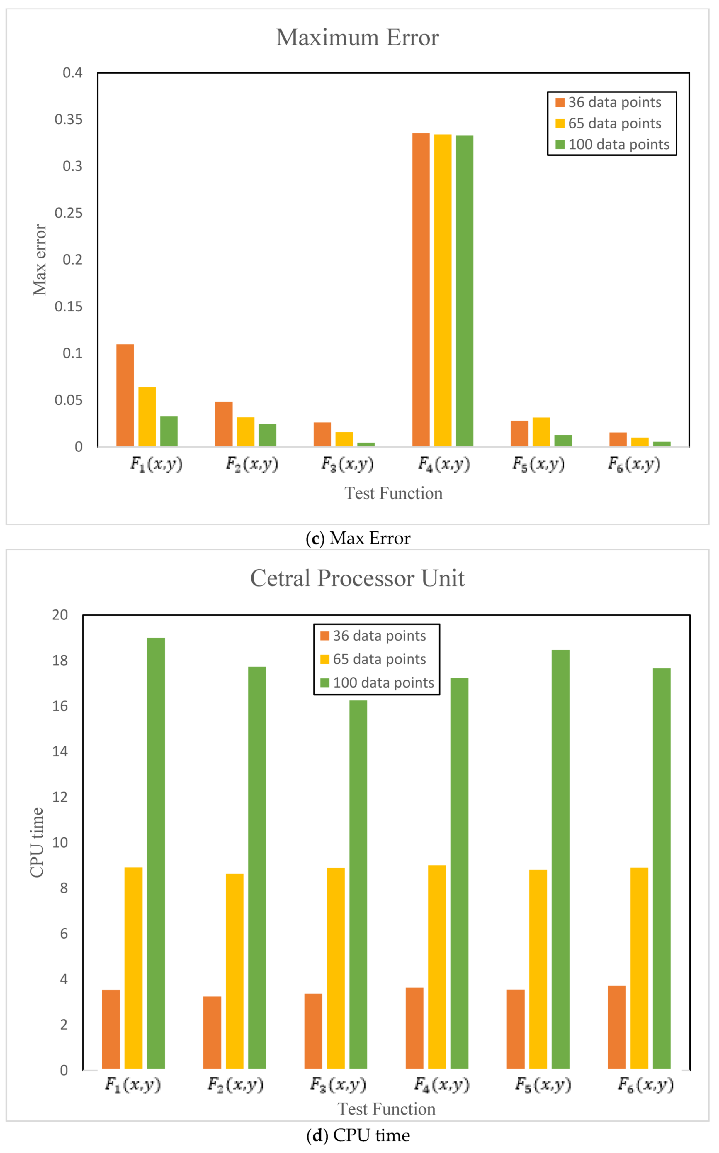
Hence, we conclude that the best scheme for scattered data interpolation is the cubic Timmer triangular patches with convex combination of Choice 1 and the Foley and Opitz [19] method to calculate the inner ordinates. Figure 24 shows the error comparison of the proposed cubic Timmer triangular patch with all test functions using the best scheme mentioned above with different datasets.

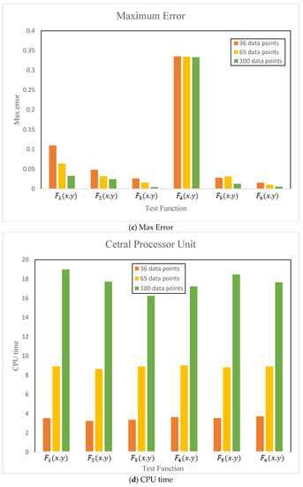
Figure 24. Comparison of the proposed method using the best schemes.

Based on Figure 24, as the number of data points increased, the errors such as RMSE and Max error will be decreased. For CPU time, when more data are used, it will take a longer time, while the comparison using R² shows that when the datasets used increases, the R² value will increase too.

Next, we compare the proposed cubic Timmer triangular scheme with the established schemes such as Karim and Saaban [21] and Goodman and Said [8]. We use 100 data points as shown in Table 4. The numerical comparisons are shown in Table 8.

Table 8. Comparison with established schemes.

Test Function	Error	100 Data Points
		Goodman and Said [8]	Karim and Saaban [21]	Proposed Scheme
${\mathit{F}}_{\mathbf{1}}\left(\mathit{x},\mathit{y}\right)$	RMSE	0.006523	0.006543	0.006660
	R2	0.999481	0.999477	0.999459
	Max error	0.032346	0.033434	0.032402
	CPU time	19.853309	19.740250	18.989466
${\mathit{F}}_{\mathbf{2}}\left(\mathit{x},\mathit{y}\right)$	RMSE	0.003486	0.003464	0.003525
	R2	0.998770	0.998786	0.998742
	Max error	0.023774	0.022634	0.024344
	CPU time	18.454829	17.937833	17.726120
${\mathit{F}}_{\mathbf{3}}\left(\mathit{x},\mathit{y}\right)$	RMSE	0.000953	0.001151	0.000960
	R2	0.999841	0.999768	0.999839
	Max error	0.004293	0.005725	0.004337
	CPU time	16.947552	16.851681	16.748355
${\mathit{F}}_{\mathbf{4}}\left(\mathit{x},\mathit{y}\right)$	RMSE	0.127205	0.127190	0.127200
	R2	0.997654	0.998057	0.997735
	Max error	0.334366	0.334366	0.334366
	CPU time	18.045273	17.586388	17.582176
${\mathit{F}}_{\mathbf{5}}\left(\mathit{x},\mathit{y}\right)$	RMSE	0.002093	0.002060	0.002159
	R2	0.999238	0.999262	0.999189
	Max error	0.012460	0.012264	0.012559
	CPU time	18.675766	18.590993	18.463083
${\mathit{F}}_{\mathbf{6}}\left(\mathit{x},\mathit{y}\right)$	RMSE	0.000873	0.000881	0.000867
	R2	0.999861	0.999858	0.999863
	Max error	0.005458	0.005458	0.005458
	CPU time	17.956438	17.777269	17.658403

From Table 8, based on RMSE, max error, and R², we can see clearly that cubic Timmer triangular patch is on par with Karim and Saaban [21] and Goodman and Said [8] schemes. However, in terms of CPU time (in seconds), the proposed scheme require smaller CPU time compared to the other established methods. Thus, we believed that the proposed cubic Timmer triangular patch is suitable to interpolate dense or big scattered datasets, since it requires less CPU time than [8] and [21].

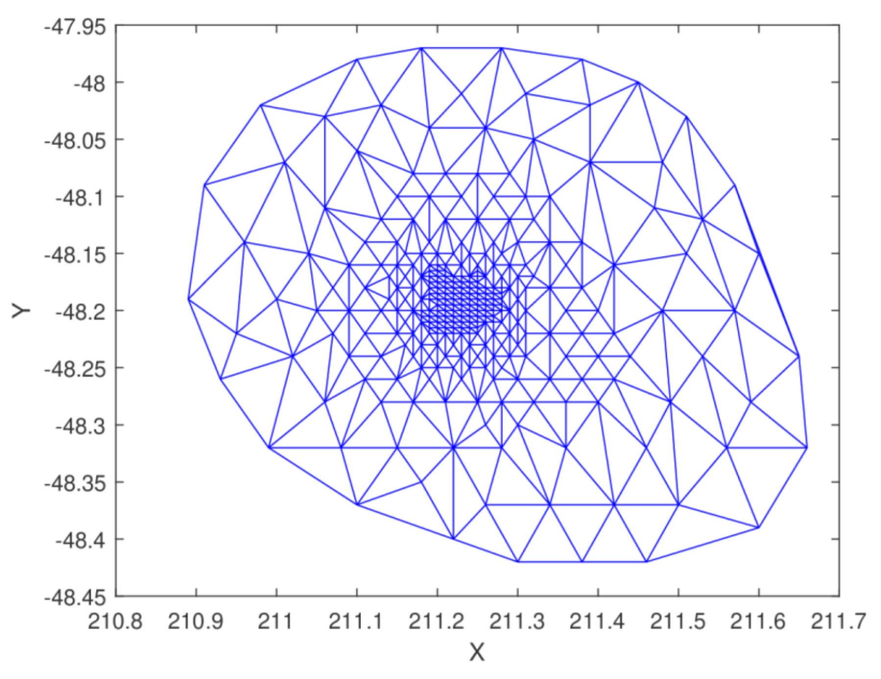
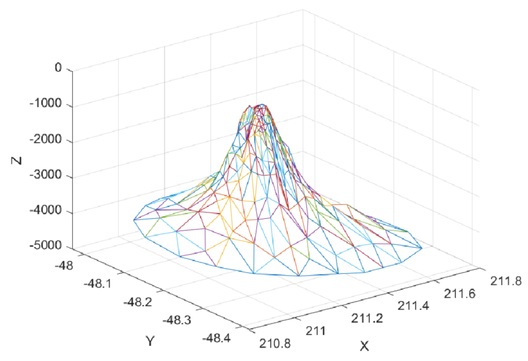
To validate this, we test the proposed cubic Timmer triangular patch scheme by using the seamount dataset obtained in MATLAB. The seamount dataset represents the surface of underwater mountain that is located at 48.2°S, 148.8°W on the Louisville Ridge in the South Pacific in 1984. The seamount data et contains 294 data points and it consists a set of longitude (X), latitude (Y), and depth-in-feet (Z), as shown in Table 9. Table 9 shows 294 data points of the seamount dataset. There are about 566 triangles. Figure 25 and Figure 26 show the Delaunay triangulation and the 3D visualization of the seamount dataset, respectively. The surface interpolation of 566 triangular patches formed by using the proposed cubic Timmer, cubic Ball, and cubic Bèzier are shown in Figure 27.

Table 9. Seamount dataset.

X	Y	Z	X	Y	Z	X	Y	Z
211.18	−47.97	−4250	211.07	−48.18	−3050	211.19	−48.215	−1100
211.28	−47.97	−4250	211.11	−48.18	−2615	211.2	−48.215	−1000
211.1	−47.98	−4250	211.15	−48.18	−1850	211.21	−48.215	−975
211.38	−47.98	−4250	211.17	−48.18	−1730	211.22	−48.215	−925
211.45	−48	−4250	211.19	−48.18	−1150	211.23	−48.215	−725
211.23	−48.01	−3900	211.2	−48.18	−1025	211.24	−48.215	−800
211.31	−48.01	−3950	211.21	−48.18	−600	211.25	−48.215	−1050
210.98	−48.02	−4250	211.22	−48.18	−900	210.95	−48.22	−4050
211.13	−48.02	−3900	211.23	−48.18	−1050	211.07	−48.22	−3700
211.39	−48.02	−4000	211.24	−48.18	−800	211.11	−48.22	−2910
211.06	−48.03	−4050	211.25	−48.18	−950	211.15	−48.22	−2150
211.51	−48.03	−4250	211.26	−48.18	−1300	211.17	−48.22	−1750
211.19	−48.04	−3700	211.27	−48.18	−1370	211.19	−48.22	−1250
211.26	−48.04	−3730	211.28	−48.18	−1450	211.2	−48.22	−1150
211.32	−48.05	−3650	211.29	−48.18	−1490	211.21	−48.22	−1125
211.1	−48.06	−3800	211.31	−48.18	−1850	211.22	−48.22	−950
211.01	−48.07	−3980	211.34	−48.18	−2575	211.23	−48.22	−950
211.39	−48.07	−3700	211.38	−48.18	−3350	211.24	−48.22	−925
211.48	−48.07	−3980	211.19	−48.185	−1300	211.25	−48.22	−1125
211.17	−48.08	−3280	211.2	−48.185	−1050	211.27	−48.22	−1350
211.21	−48.08	−3100	211.21	−48.185	−650	211.29	−48.22	−1650
211.25	−48.08	−3140	211.22	−48.185	−770	211.31	−48.22	−1750
211.29	−48.08	−3250	211.23	−48.185	−750	211.34	−48.22	−2500
210.91	−48.09	−4250	211.24	−48.185	−620	211.38	−48.22	−3025
211.57	−48.09	−4250	211.25	−48.185	−950	211.42	−48.22	−3400
211.15	−48.1	−3150	211.26	−48.185	−1150	211.16	−48.23	−2200
211.19	−48.1	−3000	211.27	−48.185	−1000	211.18	−48.23	−1850
211.23	−48.1	−2850	211.28	−48.185	−1150	211.2	−48.23	−1500
211.27	−48.1	−3000	210.89	−48.19	−4250	211.22	−48.23	−1325
211.31	−48.1	−3100	211	−48.19	−3650	211.24	−48.23	−1375
211.34	−48.1	−3220	211.14	−48.19	−2300	211.26	−48.23	−1530
211.06	−48.11	−3630	211.16	−48.19	−1940	211.28	−48.23	−1680
211.47	−48.11	−3765	211.18	−48.19	−1550	211.3	−48.23	−2000
211.13	−48.12	−3170	211.2	−48.19	−1050	211.02	−48.24	−3700
211.17	−48.12	−2875	211.21	−48.19	−675	211.09	−48.24	−3325
211.21	−48.12	−2600	211.22	−48.19	−600	211.13	−48.24	−2875
211.25	−48.12	−2600	211.23	−48.19	−590	211.17	−48.24	−2200
211.29	−48.12	−2575	211.24	−48.19	−650	211.19	−48.24	−1850
211.32	−48.12	−2950	211.25	−48.19	−800	211.21	−48.24	−1600
211.53	−48.12	−4070	211.26	−48.19	−1050	211.23	−48.24	−1900
210.96	−48.14	−3920	211.27	−48.19	−950	211.25	−48.24	−1800
211.11	−48.14	−2950	211.28	−48.19	−1000	211.27	−48.24	−1930
211.15	−48.14	−2550	211.3	−48.19	−1780	211.29	−48.24	−2000
211.19	−48.14	−2350	211.19	−48.19	−1150	211.31	−48.24	−2250
211.23	−48.14	−2195	211.2	−48.195	−850	211.36	−48.24	−2800
211.27	−48.14	−2080	211.21	−48.195	−600	211.4	−48.24	−3220
211.3	−48.14	−2450	211.22	−48.195	−570	211.44	−48.24	−3500
211.34	−48.14	−2925	211.23	−48.195	−555	211.53	−48.24	−3650
211.38	−48.14	−3125	211.24	−48.195	−580	211.65	−48.24	−4250
211.04	−48.15	−3450	211.25	−48.195	−700	211.18	−48.25	−2150
211.16	−48.15	−2110	211.26	−48.195	−750	211.2	−48.25	−1840
211.18	−48.15	−2100	211.27	−48.195	−875	211.22	−48.25	−2275
211.2	−48.15	−1760	211.28	−48.195	−1020	211.24	−48.25	−2275
211.22	−48.15	−1920	211.05	−48.2	−3275	211.26	−48.25	−2150
211.24	−48.15	−1900	211.09	−48.2	−2865	211.28	−48.25	−2250
211.26	−48.15	−1750	211.13	−48.2	−2480	210.93	−48.26	−4250
211.28	−48.15	−2110	211.15	−48.2	−2025	211.11	−48.26	−3240
211.51	−48.15	−3950	211.17	−48.2	−1375	211.15	−48.26	−2675
211.6	−48.15	−4250	211.18	−48.2	−1000	211.19	−48.26	−2100
211.09	−48.16	−2950	211.19	−48.2	−825	211.23	−48.26	−2575
211.13	−48.16	−2570	211.2	−48.2	−700	211.27	−48.26	−2400
211.15	−48.16	−1950	211.21	−48.2	−580	211.3	−48.26	−2550
211.17	−48.16	−1750	211.22	−48.2	−510	211.34	−48.26	−2820
211.19	−48.16	−1480	211.23	−48.2	−500	211.38	−48.26	−3050
211.2	−48.16	−1325	211.24	−48.2	−550	211.42	−48.26	−3400
211.21	−48.16	−1350	211.25	−48.2	−600	211.06	−48.28	−3725
211.23	−48.16	−1650	211.26	−48.2	−735	211.13	−48.28	−3120
211.25	−48.16	−1375	211.27	−48.2	−875	211.17	−48.28	−2800
211.27	−48.16	−1780	211.28	−48.2	−1150	211.21	−48.28	−3050
211.29	−48.16	−2125	211.29	−48.2	−1500	211.25	−48.28	−2925
211.31	−48.16	−2200	211.31	−48.2	−2150	211.28	−48.28	−2775
211.36	−48.16	−2940	211.36	−48.2	−3000	211.32	−48.28	−2920
211.42	−48.16	−3450	211.4	−48.2	−3380	211.36	−48.28	−3190
211.19	−48.165	−1150	211.48	−48.2	−3780	211.4	−48.28	−3260
211.2	−48.165	−1125	211.57	−48.2	−4025	211.49	−48.28	−3780
211.21	−48.165	−1150	211.18	−48.205	−950	211.59	−48.28	−4050
211.25	−48.165	−1125	211.19	−48.205	−800	211.26	−48.3	−3250
211.14	−48.17	−2250	211.2	−48.205	−740	211.3	−48.3	−3140
211.16	−48.17	−1875	211.21	−48.205	−595	210.99	−48.32	−4250
211.18	−48.17	−1340	211.22	−48.205	−595	211.08	−48.32	−3950
211.19	−48.17	−1075	211.23	−48.205	−490	211.15	−48.32	−3750
211.2	−48.17	−850	211.24	−48.205	−650	211.22	−48.32	−3630
211.21	−48.17	−850	211.25	−48.205	−748	211.28	−48.32	−3420
211.22	−48.17	−1100	211.26	−48.205	−850	211.36	−48.32	−3420
211.23	−48.17	−1375	211.27	−48.205	−1000	211.46	−48.32	−3735
211.24	−48.17	−1175	211.16	−48.21	−1700	211.56	−48.32	−4015
211.25	−48.17	−950	211.18	−48.21	−1200	211.66	−48.32	−4250
211.26	−48.17	−1300	211.19	−48.21	−1000	211.18	−48.35	−4010
211.28	−48.17	−1825	211.2	−48.21	−850	211.1	−48.37	−4250
211.3	−48.17	−1850	211.21	−48.21	−765	211.26	−48.37	−3950
211.32	−48.17	−2110	211.22	−48.21	−780	211.34	−48.37	−3850
211.19	−48.175	−1125	211.23	−48.21	−560	211.42	−48.37	−3900
211.2	−48.175	−800	211.24	−48.21	−750	211.5	−48.37	−4050
211.21	−48.175	−700	211.25	−48.21	−850	211.6	−48.39	−4250
211.22	−48.175	−1020	211.26	−48.21	−1040	211.22	−48.4	−4250
211.23	−48.175	−1175	211.27	−48.21	−1200	211.3	−48.42	−4250
211.24	−48.175	−900	211.28	−48.21	−1300	211.38	−48.42	−4250
211.25	−48.175	−900	211.3	−48.21	−1600

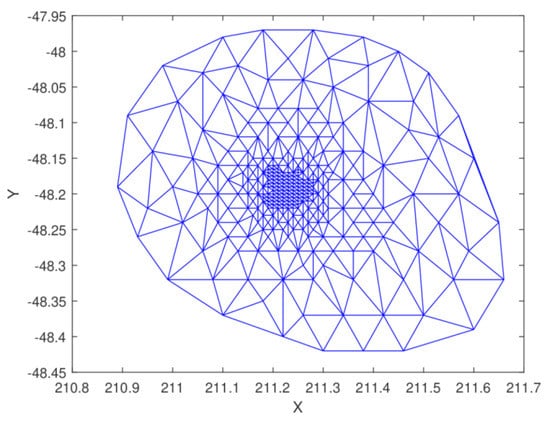
Figure 25. Delaunay triangulation of seamount dataset.

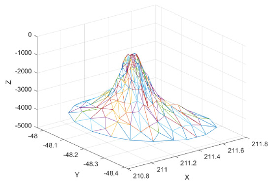
Figure 26. 3D visualization of seamount dataset.

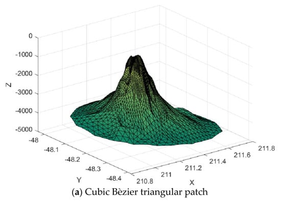
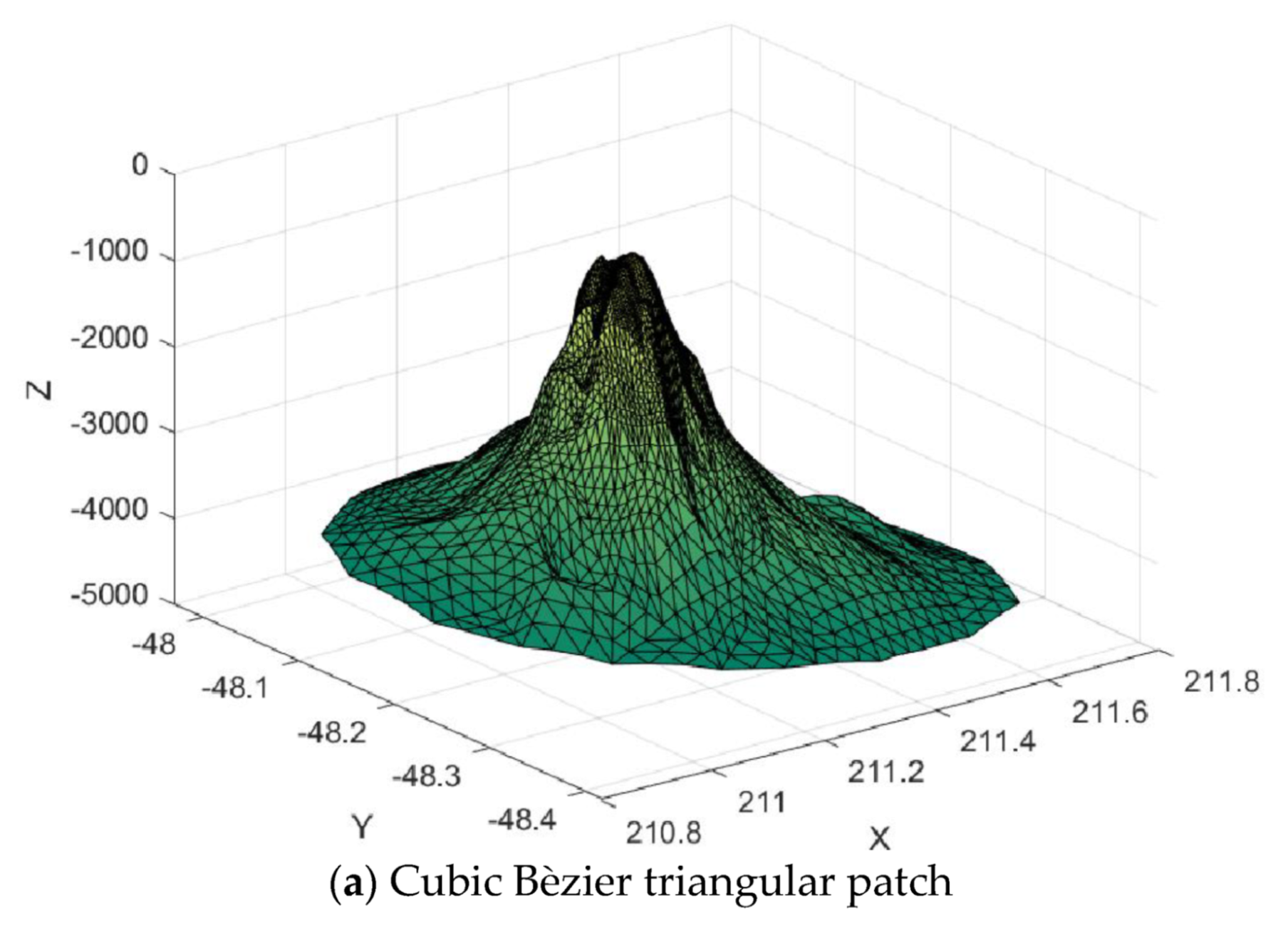
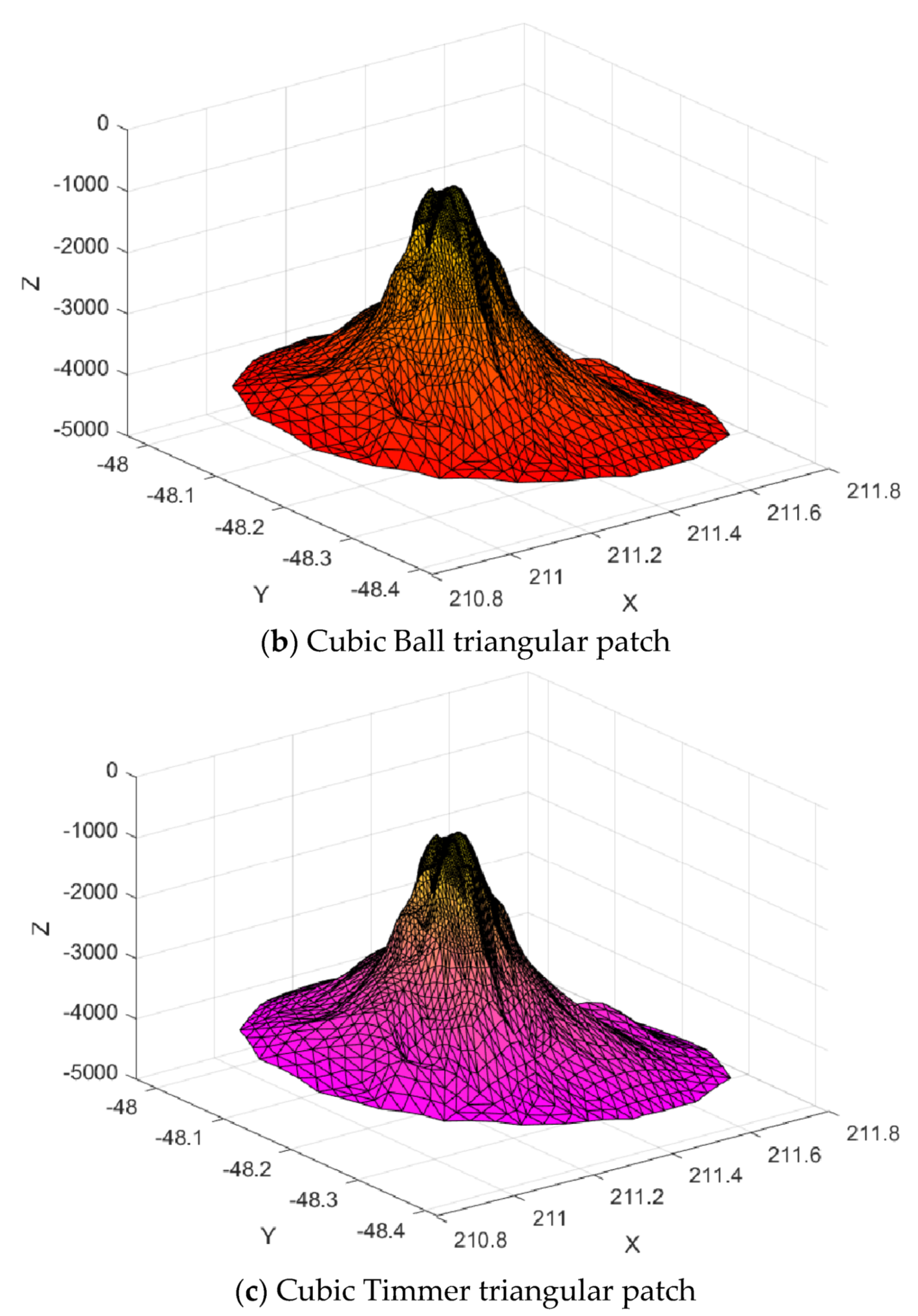
Figure 27. Surface interpolation.

Then, we calculate the CPU time (in seconds) for each of the construction of the surfaces by using different methods shown in Figure 27. CPU time taken by proposed cubic Timmer triangular patches to construct the surface of the seamount dataset is 102.3931 s. Furthermore, cubic Bèzier and Ball triangular patches required about 103.7781 s and 103.5014 s, respectively. Based on this example, we conclude that the proposed cubic Timmer triangular patch required smaller CPU time especially for big or dense scattered datasets. Furthermore, based on Renka and Brown [22], when the coefficient of determination (R²) is 0.999, the interpolation method can be considered as excellent. Therefore, from all numerical results, the proposed scheme is excellent.

6. Application on Real Data

In this section, the proposed scattered data interpolation using cubic Timmer triangular patch is tested to visualize some real datasets. We use two different datasets i.e., the rainfall data and the digital elevation data. All scattered data discussed in this section are irregularly distributed.

6.1. Visualize the Rainfall Data

First, we test the proposed scattered data interpolation scheme to visualize rainfall data. Based on our previous discussion, we apply the Foley and Opitz [19] method to calculate the inner ordinates and local scheme of Choice 1. The rainfall data sites are obtained from Malaysian Meteorology Department. The data are of average rainfall that were collected at some 25 major stations throughout Peninsular Malaysia. We have chosen the rainfall data for three different months i.e., February, March, and May 2007, as shown in Table 10. Figure 28 shows the Delaunay triangulation of rainfall data at the collected stations.

Table 10. Rainfall data.

Station	Location		Average Rainfall (mm)
	Longitude	Latitude	Feb	March	May
Chuping	100.2667	6.4833	68.6	61.0	88.0
Langkawi Island	99.7333	6.3333	49.8	40.6	166.0
Alor Setar	100.4000	6.2000	99.4	277.8	67.4
Butterworth	100.3833	5.4667	31.6	58.9	143.2
Prai	100.4000	5.3500	33.8	208.1	153.4
Bayan Lepas	100.2667	5.3000	39.8	125.2	144.4
Ipoh	101.1000	4.5833	242.4	364.2	42.6
Cameron Highlands	101.3667	4.4667	117.2	252.0	223.2
Lubok Merbau	100.9000	4.8000	62.6	156.4	98.4
Sitiawan	100.7000	4.2167	49.8	44.4	26.8
Subang	101.5500	3.1167	199.0	329.2	68.2
Petaling Jaya	101.6500	3.1000	139.8	321.0	196.2
KLIA (Sepang)	101.7000	2.7167	78.6	186.2	188.8
Melaka	102.2500	2.2667	62.4	113.8	183.4
Batu Pahat	102.9833	1.8667	219.0	182.0	195.0
Kluang	103.3100	2.0167	39.4	92.4	130.2
Senai	103.6667	1.6333	176.3	148.6	296.0
Kota Bahru	102.2833	6.1667	7.0	115.2	109.2
Kuala Krai	102.2000	5.5333	16.6	166.0	238.7
Kuala Terengganu	103.1000	5.3833	0.2	121.0	64.8
Kuantan	103.2167	3.7833	35.2	79.2	270.4
Batu Embun	102.3500	3.9667	103.2	146.2	256.2
Temerloh	102.3833	3.4667	25.6	114.2	324.2
Muadzam Shah	103.0833	3.0500	85.0	131.6	204.8
Mersing	103.8333	2.4500	16.4	183.4	196.2

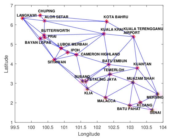
Figure 28. Delaunay triangulation of rainfall data.

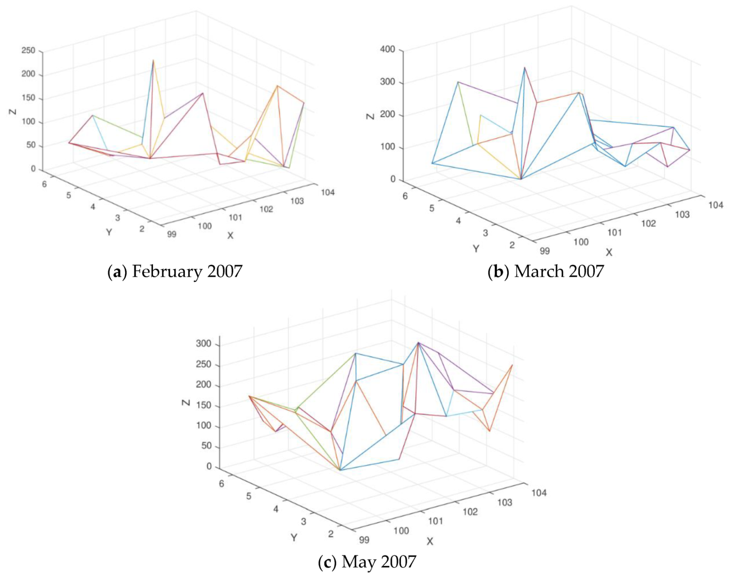
Figure 29 shows the 3D linear interpolant of the rainfall data for each month. The surface of rainfall distribution in Malaysia of cubic Timmer triangular patches according to each month is shown in Figure 30.

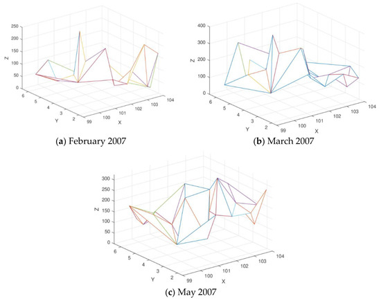
Figure 29. 3D Linear Interpolant of the rainfall data.

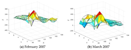
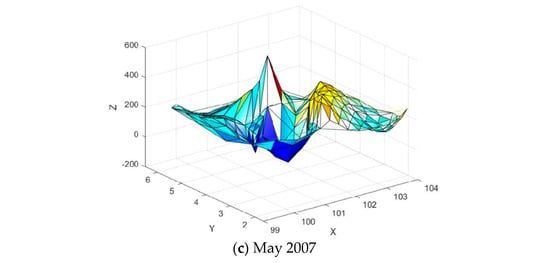
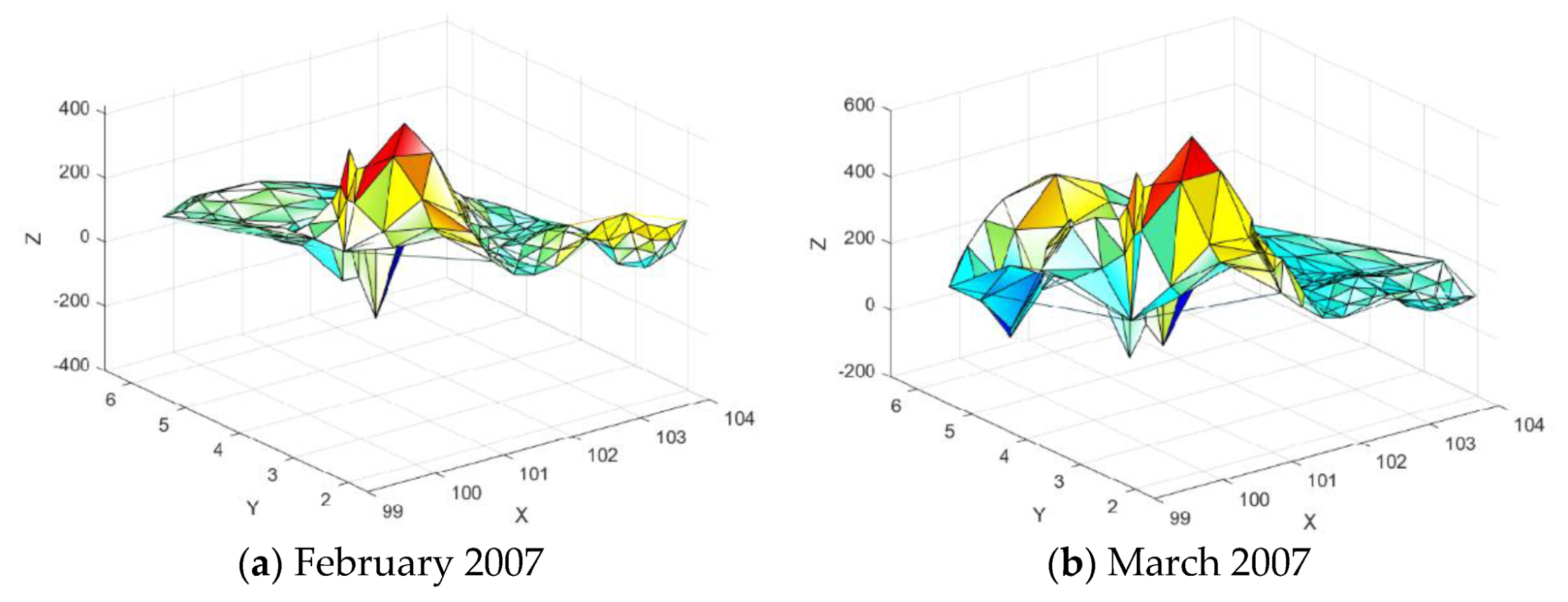
Figure 30. Surface Interpolation using the proposed scheme.

Meanwhile, Table 11 shows all the surface interpolations show that the minimum value of the average rainfall less than zero as shown in Table 11.

Table 11. Minimum value (mm).

Average Rainfall (mm)	Minimum Value (mm)
Feb	−259.9196
March	−165.0851
May	−71.3284

6.2. Visualize the Digital Elevation Data of Kalumpang Agricultural Station

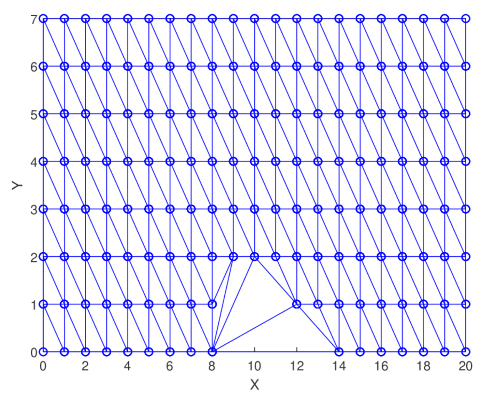
Next, we test the proposed scattered data interpolation scheme to visualize the 160 digital elevation data of Kalumpang Agricultural Station (3° 38′ N, 101.34′ E) located about 90 km northeast of Kuala Lumpur, Malaysia (refer to z values in Table 12). We also apply the Foley and Opitz [19] method and Choice 1 to calculate the inner ordinates and local scheme of the proposed cubic Timmer triangular patch. Figure 31 shows the Delaunay triangulation for all 160 data points.

Table 12. Digital elevation data of Kalumpang Agricultural Station.

X	Y	Z	X	Y	Z	X	Y	Z
0	0	73.70	6	6	81.40	14	4	83.60
0	1	75.00	6	7	82.90	14	5	83.40
0	2	76.20	7	0	72.25	14	6	84.40
0	3	77.40	7	1	74.40	14	7	85.45
0	4	78.60	7	2	75.85	15	0	79.00
0	5	79.70	7	3	77.40	15	1	80.30
0	6	80.80	7	4	79.10	15	2	82.20
0	7	81.70	7	5	80.50	15	3	82.20
1	0	73.25	7	6	81.60	15	4	83.80
1	1	74.60	7	7	83.50	15	5	83.90
1	2	75.80	8	0	72.80	15	6	84.75
1	3	77.25	8	1	74.70	15	7	85.70
1	4	78.45	8	2	76.00	16	0	79.75
1	5	79.70	8	3	77.80	16	1	81.60
1	6	80.85	8	4	79.60	16	2	82.70
1	7	82.20	8	5	80.95	16	3	82.80
2	0	72.90	8	6	82.15	16	4	84.25
2	1	74.10	8	7	83.40	16	5	84.25
2	2	75.60	9	2	77.00	16	6	85.20
2	3	77.00	9	3	78.00	16	7	85.90
2	4	78.60	9	4	80.25	17	0	80.40
2	5	79.60	9	5	81.40	17	1	81.50
2	6	81.15	9	6	82.50	17	2	83.30
2	7	82.30	9	7	83.80	17	3	83.30
3	0	72.25	10	2	77.55	17	4	84.75
3	1	73.80	10	3	79.20	17	5	84.75
3	2	75.70	10	4	80.70	17	6	85.45
3	3	76.80	10	5	81.75	17	7	86.10
3	4	78.40	10	6	83.15	18	0	81.20
3	5	79.80	10	7	84.15	18	1	82.10
3	6	81.10	11	2	78.40	18	2	83.80
3	7	82.40	11	3	79.80	18	3	83.80
4	0	72.20	11	4	81.20	18	4	85.15
4	1	73.70	11	5	82.30	18	5	85.10
4	2	75.50	11	6	83.45	18	6	85.60
4	3	77.00	11	7	84.65	18	7	86.20
4	4	78.40	12	1	77.50	19	0	81.70
4	5	79.80	12	2	80.40	19	1	82.75
4	6	81.05	12	3	80.40	19	2	84.25
4	7	82.45	12	4	82.80	19	3	84.25
5	0	71.15	12	5	82.80	19	4	85.40
5	1	73.75	12	6	83.70	19	5	85.40
5	2	75.75	12	7	84.70	19	6	85.80
5	3	77.15	13	1	78.50	19	7	86.30
5	4	78.50	13	2	80.80	20	0	82.50
5	5	79.90	13	3	80.80	20	1	82.80
5	6	81.40	13	4	83.50	20	2	84.60
5	7	82.60	13	5	83.50	20	3	84.60
6	0	72.15	13	6	84.00	20	4	85.10
6	1	73.75	13	7	85.00	20	5	85.60
6	2	75.80	14	0	78.50	20	6	86.00
6	3	77.25	14	1	79.30	20	7	86.50
6	4	78.80	14	2	81.60
6	5	80.20	14	3	81.10

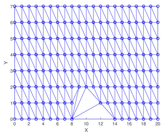
Figure 31. Delaunay triangulation for digital elevation data.

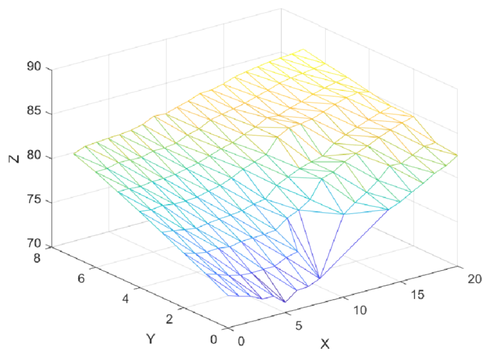
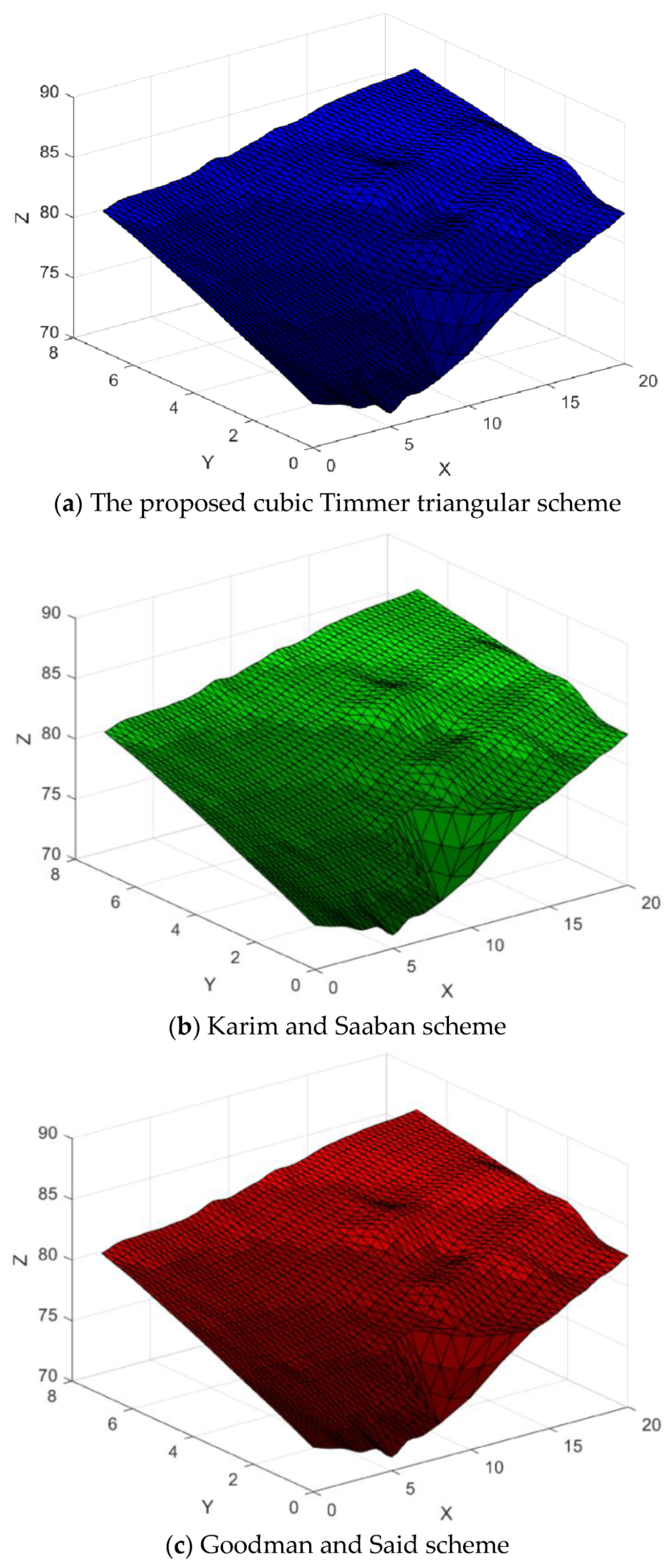
Figure 32 shows the 3D linear interpolant of the data points. The interpolating surfaces using the proposed cubic Timmer, Karim and Saaban [21], and Goodman and Said [8] schemes are illustrated in Figure 33. The final interpolating surface is constructed by combing all 269 triangular patches.

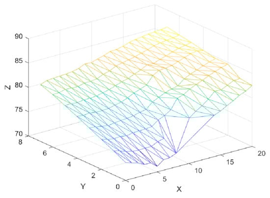
Figure 32. 3D linear interpolant for digital elevation data.

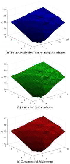
Figure 33. Surface Interpolation.

Based on Figure 33, all interpolating surface are visually pleasing. However, we can compare the effectiveness of the proposed scheme by calculating the CPU time (in seconds). The proposed cubic Timmer triangular scheme took about 33.6956 s to construct the surface. Furthermore, the Karim and Saaban [21] scheme required 33.8426 s while the Goodman and Said [8] scheme required 33.9239 s to interpolate the surface of digital elevation data. Hence, we can conclude that the proposed cubic Timmer triangular scheme is the best scheme in terms of CPU time compared to other schemes.

7. Conclusions and Future Work

In this paper, the cubic Timmer triangular patches, as implemented in Ali et al. [16], is applied to interpolate the scattered data. Goodman and Said [8] and Foley and Opitz [19] schemes are used in order to calculate the inner ordinates for each local scheme. It is observed that the cubic Timmer triangular patches offer lower CPU time (computational cost) as compared to the cubic Bezier and Ball triangular patches methods. Moreover, the simulation error shows that the cubic Timmer triangular patches have the same values as obtained from Goodman and Said schemes. In addition, we infer from the obtained results that the cubic Timmer triangular patches give better results as compared to some established schemes when the datasets are increasing. Therefore, we can preserve the positivity of the rainfall data by constructing the shape preservation of cubic Timmer triangular patches in our main studies in future.

References

- Amato, F.; Moscato, V.; Picariello, A.; Sperlí, G. Recommendation in social media networks. In Proceedings of the 2017 IEEE Third International Conference on Multimedia Big Data (BigMM), Laguna Hills, CA, USA, 19–21 April 2017; pp. 213–216. [Google Scholar]
- Karim, S.A.B.A.; Saaban, A. Visualization Terrain Data Using Cubic Ball Triangular Patches. In Proceedings of the MATEC Web of Conferences, 18–19 September 2018; Volume 225, p. 06023. [Google Scholar]
- Ni, H.; Li, Z.; Song, H. Moving least square curve and surface fitting with interpolation conditions. In Proceedings of the 2010 International Conference on Computer Application and System Modeling (ICCASM 2010), Taiyuan, China, 22–24 October 2010; Volume 13, pp. V13–V300. [Google Scholar]
- Ali, F.A.M.; Karim, S.A.A.; Dass, S.C.; Skala, V.; Saaban, A.; Hasan, M.K.; Ishak, H. Efficient Visualization of Scattered Energy Distribution Data by Using Cubic Timmer Triangular Patches. In Energy Efficiency in Mobility Systems; Sulaiman, S.A., Ed.; Springer: Singapore, 2020; pp. 145–180. [Google Scholar]
- Awang, N.; Rahmat, R.W. Reconstruction of Smooth Surface by Using Cubic Bezier Triangular Patch in Gui. Malays. J. Ind. Technol. 2017, 2, 61–69. [Google Scholar]
- Cavoretto, R.; Rossi, A.D.; Dell’Accio, F.; Tommaso, F.D. Fast computation of triangular Shepard interpolants. J. Comput. Appl. Math. 2019, 354, 457–470. [Google Scholar] [CrossRef]
- Grise, G.; Meyer-Hermann, M. Surface reconstruction using Delaunay triangulation for applications in life sciences. Comput. Phys. Commun. 2011, 182, 967–977. [Google Scholar] [CrossRef]
- Goodman, T.N.; Said, H. A Triangular Interpolant Suitable for Scattered Data Interpolation. Commun. Appl. Numer. Methods 1991, 7, 479–485. [Google Scholar] [CrossRef]
- Hussain, M.Z.; Hussain, M. Shape preserving scattered data interpolation. Eur. J. Sci. Res. 2009, 25, 151–164. [Google Scholar]
- Hussain, M.Z.; Sarfraz, M. Monotone piecewise rational cubic interpolation. Int. J. Comput. Math. 2009, 86, 423–430. [Google Scholar] [CrossRef]
- Hussain, M.Z.; Hussain, M. C1 positivity preserving scattered data interpolation using rational Bernstein-Bézier triangular patch. J. Appl. Math. Comput. 2011, 35, 281–293. [Google Scholar] [CrossRef]
- Karim, S.A.A. Monotonic Interpolating Curves by Using Rational Cubic Ball Interpolation. Appl. Math. Sci. 2014, 8, 7259–7276. [Google Scholar] [CrossRef]
- Karim, S.A.A.; Saaban, A.; Hasan, M.K.; Sulaiman, J.; Hashim, I. Interpolation using Cubic Bèzier Triangular Patches. Int. J. Adv. Sci. Eng. Inf. Technol. 2018, 8, 1746–1752. [Google Scholar] [CrossRef]
- Ibraheem, F.; Hussain, M.Z.; Bhatti, A.A. C¹ Positive Surface over Positive Scattered Data Sites. PLOS ONE 2015, 10, e0120658. [Google Scholar] [CrossRef] [PubMed]
- Su, X.; Sperli, G.; Moscato, V.; Picariello, A.; Esposito, C.; Choi, C. An Edge Intelligence Empowered Recommender System Enabling Cultural Heritage Applications. IEEE Trans. Ind. Inform. 2019, 15, 4266–4275. [Google Scholar] [CrossRef]
- Ali, F.A.M.; Karim, S.A.A.; Dass, S.C.; Skala, V.; Saaban, A.; Hasan, M.K.; Ishak, H. New cubic Timmer triangular patches with C1 and G1continuity. J. Teknol. 2019, 81, 1–11. [Google Scholar]
- Timmer, H.G. Alternative representation for parametric cubic curves and surfaces. Comput.-Aided Des. 1980, 12, 25–28. [Google Scholar] [CrossRef]
- Goodman, T.N.T.; Said, H.B.; Chang, L.H.T. Local derivative estimation for scattered data interpolation. Appl. Math. Comput. 1995, 68, 41–50. [Google Scholar] [CrossRef]
- Foley, T.A.; Opitz, K. Hybrid cubic Bézier triangle patches. In Mathematical Methods in Computer Aided Geometric Design II; Academic Press: New York, NY, USA, 1992; pp. 275–286. [Google Scholar]
- Awang, N.; Rahmat, R.W.; Sulaiman, P.S.; Jaafar, A. Delaunay Triangulation of a missing points. J. Adv. Sci. Eng. 2017, 7, 58–69. [Google Scholar]
- Karim, S.A.A. Shape Preserving by Using Rational Cubic Ball Interpolant. Far East J. Math. Sci. 2015, 96, 211–230. [Google Scholar]
- Renka, R.J.; Brown, R. Algorithm 792: Accuracy Tests of ACM Algorithms for Interpolation of Scattered Data in the Plane. ACM Trans. Math. Softw. 1999, 25, 78–94. [Google Scholar] [CrossRef]
© 2020 by the authors. Licensee MDPI, Basel, Switzerland. This article is an open access article distributed under the terms and conditions of the Creative Commons Attribution (CC BY) license (http://creativecommons.org/licenses/by/4.0/).