Abstract
With the improvement of people’s living standards and entertainment interests, theme parks have become one of the most popular holiday places. Many theme park websites provide a variety of information, according to which tourists can arrange their own schedules. However, most theme park websites usually have too much information, which makes it difficult for tourists to develop a tourism planning. Therefore, the theme park routing problem has attracted the attention of scholars. Based on the Traveling Salesman Problem (TSP) network, we propose a Time-Dependent Theme Park Routing Problem (TDTPRP), in which walking time is time-dependent, considering the degree of congestion and fatigue. The main goal is to maximize the number of attractions visited and satisfaction and to reduce queues and walking time. To verify the feasibility and the effectiveness of the model, we use the Partheno-Genetic Algorithm (PGA) and an improved Annealing Partheno-Genetic Algorithm (APGA) to solve the model in this paper. Then, in the experimental stage, we conducted two experiments, and the experimental data were divided into real-world problem instances and randomly generated problem instances. The results demonstrate that the parthenogenetic simulated annealing algorithm has better optimization ability than the general parthenogenetic algorithm when the data scale is expanded.
1. Introduction
With the improvement of people’s living standards and material level, people’s daily lives are no longer solely focused on the pursuit of food and clothing but include more spiritual pursuits. Holiday outings have become a common form of entertainment for modern people. Among them, theme parks have become the best place for short-term travel [1]. Some famous theme parks such as Tokyo Disneyland and Universal Studios Osaka attract millions of visitors every year, which shows that, as people’s living standards improve, people’s demand for the entertainment industry is also increasing. However, several issues in theme parks need to be resolved. For example, for popular attractions, tourists need to endure long queues, which may take two or three hours. In addition, since most theme parks are large in size and populated, tourists spend a lot of time walking and queuing. Therefore, quickly planning the best way to enjoy the theme park with limited time and energy, avoiding congestion, and enjoying as many attractions as possible has become the most important concerns for tourists. Moreover, for the managers of theme parks, the degree of satisfaction of tourists is fundamental to the sustainable development of the theme park. The higher the evaluation of tourists is, the more other tourists will be attracted to the theme park. In contrast, if the degree of satisfaction of tourists is very low, the development of the theme park will be restricted.
In 2003, the theme park problem was defined by Kawamura et al. [2], that is, in a theme park with multiple attractions, tourists visit the attractions as individuals or groups to minimize congestion and satisfaction. In addition, they developed a coordinated scheduling algorithm based on large-scale user support to solve this problem, proving that the average waiting time and congestion in theme parks can be reduced by guiding tourist groups, and the average satisfaction of group visitors can be improved. In short, the problem of theme parks is to maximize personal or crowd satisfaction using management rules and planned timetables. Considering the group users, Yasushi et al. [3] developed networks for theme park issues, such as small world networks and scale-free networks. Simulation experiment results show that congestion can be greatly relieved, and satisfaction can be further improved.
Most previous studies involving the theme park problem focus on large-scale travel scheduling for group users. However, differently, in this paper, we aim to help individual users avoid congestion and improve the degree of satisfaction of the visitors in the theme park. We can call this kind of problem theme park routing problem (TPRP). Thus far, route planning for individual users is usually divided into two categories:
- One category aims to find an efficient route among the chosen attractions [4].
- The other is to select some attractions to visit and maximize the obtained total score for visited attractions during a limited time, where origin and destination are appointed in advance [5].
The research in this paper belongs to the second category, which does not need to specify the attractions in advance. Tsai et al. [6] developed a route recommendation system where the recommended route satisfies visitor requirements using previous tourists’ favorite experiences. Lee et al. [7] presented an ontological recommendation for a multi-agent for Tainan City travel, including a context decision agent and a travel route recommendation agent. Lim, K. et al. [8] proposed an algorithm called PersTour for recommending personalized tours using Points of Interest (POI) popularity and user interest preferences, which are automatically derived from real-life travel sequences based on geo-tagged photos. Mor, M. et al. [9] developed a bi-directional constrained pathfinder nearest neighbor route calculation algorithm to compute routes that visit the most popular touristic locations among photographers. Gionis, A. et al. [10] presented two alternative instantiations of a framework for generating customized tour recommendations as a paradigm of an intelligent urban navigation service. Sengupta, L. et al. [11] considered three different strategies for selecting the starting location and compared their effectiveness regarding optimizing tour length. Hirotaka et al. [12] proved the tour recommendation problem can be solved as the integer programming problem using a similar formulation as used in the traveling salesman problem (TSP). Matsuda et al. [13] established a simple model of the optimal sightseeing routing problem and solved the model with the exact algorithm and the heuristic algorithm, respectively.
From the perspective of mathematical modeling, our problem can be described as follows. A set of points is given, along with associated scores and a connecting network. Under this assumption, a path needs to be found between the specified starting point and end point to maximize the total score at a given time. Through the above description, we find that this kind of problem can be attributed to the TSP [14]. It should be noted that, due to the limited time, it is impossible to select all points, and some points should be discarded. Subsequently, this problem is also called the selective traveling salesperson problem (STSP) [15] or traveling salesman problem with profits [16], which is a generalized traveling salesman problem in which profit is associated with each vertex and only some vertices can be visited due to time constraints [17]. The STSP is also known as the orienteering problem [18] and the maximum collection problem [19]. As the STSP is an Non-Deterministic Polynomial (NP) hard problem, the exact algorithms are very time-consuming, thus most researchers focus on heuristic algorithms, such as the Tabu search (TS) heuristic algorithm [20,21] or the ant colony optimization (ACO) approach [22].
The major weakness of the previous research is that only static route networks are constructed, but the change of time that leads to a change in the next journey is not considered. Considering this problem, Bouzarth et al. [23] set the service time as time-dependence but did not consider that the travel times between two vertices are stochastic functions that depend on the department time from the first vertex. Moreover, the previous studies are all single objective functions, and there are few cases of solving multi-objective problems at the same time. The algorithm research of routing optimization is mainly carried out under the condition of static networks, and there is less research using dynamic networks.
Unlike previous research, we first propose to minimize total walking and queuing time and maximize the number of attractions and the degree of satisfaction, which has a multi-objective function. Then, we consider the walking time of time dependence [24,25]. Second, we introduce two algorithms in detail to solve this problem. Finally, in the experimental stage, we use real-world problem instances and randomly generated problem instances and analyze the experimental results to prove the correctness of the model and the effectiveness of the algorithm.
2. Time-Dependent Theme Park Routing Problem Based on Multi-Objectives
2.1. Problem Description
Let = (𝑁, 𝐴) be a connected digraph with node set 𝑁 = {1,2...,𝑛} and arc set 𝐴 = {(,) | , ∈ 𝑁, }, where node 1 is the starting point, and n is the end point. In the time-dependent theme park routing problem, each node represents an attraction in the theme park. What is associated with each node is a utility score and a function of dwelling time, which is related to arrival time, queuing time, and time at the attraction. When visitors enter from the designated entrance, they should find the most satisfactory route to the attraction and cannot leave the exit after the designated time In this process, the objective of visitors is to find a route that starts from node 1 and ends at node n before , such that the total utility collected by all visited nodes in the route is maximized and the number of nodes experienced is maximized but the dwelling time is minimized.
Assume that the distance between the two attractions () is , and the walking times that the visitors need to cover this section () in two connected time periods are and , respectively, and is the boundary time of the two time periods. It should be noted that stands for time period and stands for time point. The walking time of the visitor in the section () is different for different time periods. The arrival time at node is , the queuing time at node is , the time spent at the attraction at node is , and the departure time for node is . If , the walking time to cover this section in the preceding period is ; if , the whole walking process is completed in the following period, and the corresponding walking time is . Only when is the walking time between and . Assume that the walking distances of the visitor in the preceding and the following time periods are and , corresponds to the travel distance of tourists in period, and corresponds to the travel distance of tourists in period. The total walking time is . Subsequently, the time is for visitors to cover , and the time for visitors to cover d2 is:
Therefore, the total walking time from the node m to the node n is , and the arrival time for node is:
As can be seen from the Equation (1), the time for arriving at the node is an increasing function of the departure time .
Assume that the playing time in one day is divided into time periods, then [] represents the time period . After the visitor arrives at attraction , the queuing time and the time spent at the attraction are allowed before the visitor departs from attraction . Let be the walking time from node to node during period (regardless of the period crossing), and let be the time that the visitor walks from node to node . For any section (), there are two possibilities:
- The visitor walks from node to node without crossing the time period ;
- The visitor walks from node m to node , crossing from period to period .
The corresponding mathematical formulations are as follows:
2.2. Model
Based on the questions raised, we consider the following assumptions:
- The queuing time of attractions is acquired according to the real queuing time of the attraction (e.g., Disney Resort and Universal Studios).
- The time spent at each attraction is given in advance.
- Routes exist between any two attractions.
- The preference of visitors for each attraction is pregiven.
The time-dependent theme park routing problem model contains the following parameters:
- N: Set of attractions
- : Index of attraction m, m∈N
- : Entrance time
- : Departure time
- P: The number of time periods in one day
- : Index of the time period,
- Weights of the functions , in which the sum of three weights is equal to 1
- Xm: If attraction m is selected, = 1; otherwise, = 0, which is a decision variable
- : The route from node m to node n with the visitor departs from node m in period is selected, it takes 1; 0 otherwise
- : Queuing time for attraction m
- : Playing time spent at attraction m
- : Walking time of visitor departing node in time period to node
- : Time for visitor walking from node to node in period (regardless of the time period crossing)
- : Departure time for attraction m
- : Arrival time for attraction m
- : Utility that the customer obtained from node m
- : The conversion factors of utility in term of cost
There are three objectives involved: maximize the number of attractions, maximize the satisfaction of the visitors, and minimize walking time and queuing time.
- Most tourists want to enjoy as many attractions as possible in the theme park within a limited time. Therefore, we consider the maximum number of attractions visited in a day, and the calculation formula is as follows:
- Most tourists hope to get as much satisfaction as possible in the theme park within a limited time. Therefore, we consider the maximum satisfaction of tourists in a day, the formula is as follows:
- For most tourists, they want to spend as much time as possible on each attraction, instead of moving on and queuing to find other attractions. Therefore, we considered the minimum walking time and the queuing time between attractions in a day; the calculation formula is as follows:
Finally, the overall mathematical model is established as follows:
The objective Equation (2) can maximize the attractiveness and the practical value (satisfaction) of the project and minimize queue time and walking time. Equation (3) ensures that the departure time from the theme park shall not exceed the preset departure time. Equations (4)–(6) are general constraints of TSP. The first two constraints restrict each scenic spot to be visited exactly once, and the last constraint is the sub-trip elimination constraint. Equations (7) and (8) are the domain of variables.
3. Algorithm
In order to solve the model better, we use two different methods to compare.
3.1. Parthenogenetic Algorithm (PGA)
The parthenogenetic algorithm (PGA) is an improved GA which was put forward by Li and Tong in 1999 [26]. Unlike classic GA, PGA performs its operations based on another chromosome other than two chromosomes and does not include a crossover operator. Due to its professionalism, PGA can successfully solve specific problems. Although PGA can overcome the “premature” problem of conventional GA, it is more suitable for handling chromosomes of different lengths.
The algorithm uses new genetic operators, namely permutation operators, shift operators, and inversion operators. They are characterized by simple genetic operations, which reduces the requirement for initial population diversity and avoids “premature convergence”. Therefore, this algorithm is very suitable for solving optimization problems.
3.1.1. Solution Representation
In PGA, each solution is represented by a chromosome, and each chromosome contains multiple variants, namely genes. Here, each gene represents the attraction of a theme park. Different arrangements of attractions require different solutions. In this study, chromosomes can be indicated as follows:
where A is a chromosome, and expresses the gene.
3.1.2. Evolution Operators
(1) Permutation operator. In this study, the permutation operator includes two modes: the first is a single-point translocation, where the positions of two genes on the same chromosome can be interchanged; the second is a multi-point translocation, where the positions of two genes on the same chromosome are exchanged. The replacement operators of the above two modes can generate new chromosomes according to the replacement probability. Examples of single-point transposition and multi-point transposition are as follows. Note that B and B’ are produced by single-point and multiple-point translocation of A chromosome, respectively.
(2) Shift operator. The shift operator refers to randomly selecting a substring in the chromosome according to the shift probability, the gene of the substring is shifted one bit backward, and the last gene is located at the first position of the substring. Similarly, the shift operator includes two shift modes: single-point shift and multi-point shift operation. In the example below, H is a chromosome including multiple genes . I and I’ are chromosomes obtained by performing single-point shift and multi-point shift operations on H, respectively.
(3) Inversion operator. The inversion operator refers to the process of continuously inverting the head and the end genes in the substring of the chromosome according to the inversion probability, wherein the selected substring and its length are randomly selected. Inversion operators can also be divided into single-point inversion and multi-point inversion. For example, assume M is a chromosome including multiple genes . Based on the operations of single-point and multi-point inversions for chromosome M, we can obtain the chromosomes N and N’. The above procedures can be seen as follows.
3.1.3. Algorithm Flow
The procedures of the parthenogenetic algorithm are summarized as follows:
Step 1: Coding. Serial number coding is used in parthenogenetic algorithm.
Step 2: Initialization. A feasible solution is randomly generated as the initial population.
Step 3: Fitness function. The fitness function is the evaluation standard of the path plan, which represents the survival ability of the genetic individual. Here, we set the objective function as the fitness function.
Step 4: Select. The resulting population is divided into several groups evenly. In this study, every four individuals formed a group. The best individuals in each group will be directly retained as the next generation population.
Step 5: Parthenon-genetic. Realize replacement, shift, and inversion operations. Among the remaining individuals, random methods are used to select genes and gene strings. After that, the three newly generated individuals in each group will be inherited to the next generation.
Step 6: Calculate the fitness of the newly generated population.
Step 7: Determine whether the termination conditions are met. When the maximum number of iterations is reached, go to step 8. Otherwise, go to step 4.
Step 8: Return the optimal solutions and stop the algorithm.
The flow chart is shown in Figure 1:
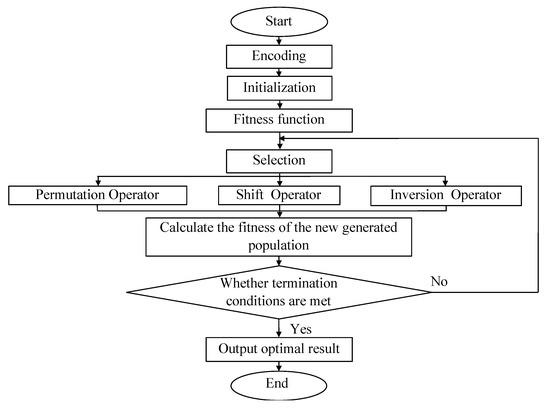
Figure 1.
The flow chart of the parthenogenetic algorithm (PGA).
3.2. Annealing Parthenogenetic Algorithm (APGA)
The global optimization ability of genetic algorithm is strong, but the local optimization ability is insufficient. The simulated annealing algorithm is strong in local optimization but weak in global optimization ability. Therefore, the evolution mechanism of simulated annealing algorithm can be integrated into genetic algorithm to enhance its local optimization ability [27].
The basic idea of simulated annealing algorithm was originated from the physical annealing process in real life. The optimal solution is acquired by abstracting the process of cooling and heating isothermals from the real physical annealing process. The local optimization ability of the algorithm is ensured using a greedy strategy and its special Metropolis criterion [28].
Li Liu et al. [29] proposed a new method combining simulated annealing (SA) and genetic algorithm (GA) to solve the problem of bus route design and frequency setting for a given road network with fixed bus stops and driving demands.
The simulated annealing method has a fault-tolerant ability and can accept inferior solutions with a certain probability. The probability is called the probability of the acceptance of the new solution, and its degree is influenced by the current temperature and the fitness difference of new and old solutions [30]. The general trend is that the lower the temperature, the lower the probability of acceptance, the larger the difference, the lower the probability of acceptance. The above can be represented by a mathematical formula, as shown in Equation (9):
refers to the fitness of the new chromosome, and refers to the fitness of the individual parent chromosome. T is the current temperature, and an initial temperature and cooling coefficient are set at the beginning of the genetic operation. As the iteration proceeds, the initial temperature decreases continuously. At the end of the iteration, because the temperature is already very low, the probability of accepting the new solution is almost zero. A random number between 0 and 1 is generated after acquiring the probability of acceptance. A new solution is not accepted if the number is greater than the probability of acceptance but accepted if it is smaller than . The selection method of the probability of acceptance is also called the Metropolis criterion.
Metropolis criterion based on a simulated annealing algorithm certainly accepts inferior solutions while accepting elegant solutions so as to ensure population diversity and further avoid the possibility that the algorithm is stuck in the optimal local solution.
Therefore, after the new solution is generated by the evolution operation of genetic algorithm, the Metropolis criterion can be used to determine if the new solution is reserved; the optimization steps are as follows:
Step 1: Encoding. A serial number encoding is adopted in the parthenogenetic algorithm.
Step 2: Initialization. Generate feasible solutions as the initial population randomly.
Step 3: Fitness function. Fitness function is the evaluation criterion of the path scheme, and it represents the viability of genetic individuals. Here, we set the objective function as the fitness function.
Step 4: Selection. The resulting population is divided into several groups evenly. In this study, every four individuals formed a group. The best individuals in each group were directly retained as the next generation population.
Step 5: Parthenogenetic. Implement permutation, shift, and inversion operations. Among the remaining individuals, random methods are used to select genes and gene strings. Then, inherit the three newly generated individuals from each group to the next generation.
Step 6: Calculate the fitness of the newly generated population.
Step 7: Mix new and original populations. First, reserve the best individuals in the. two populations and calculate the average fitness. Then, select one among the mixed population (except for the optimal individual) at random. If the individual is better than the average value, reserve it; otherwise, check whether it meets the M criterion. If satisfied, reserve it. If not, discard it. Operate in this way until the population of the quantity, which is the same as the original individuals, and then stop.
Step 8: Determine whether termination conditions are met. When the maximum iteration is reached, go to Step 8. Otherwise, go to Step 4.
Step 9: Return the optimal solutions and stop the algorithm.
The algorithm flow chart is shown in Figure 2:
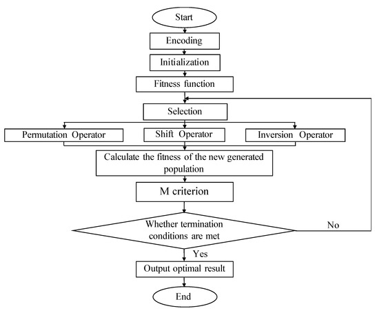
Figure 2.
The flow chart of annealing parthenogenetic algorithm (APGA).
4. Discussion Computation Results
In the experiment, we use two kinds of theme parks with different scales as examples. First, we use the Tokyo Disney Sea with 28 attractions as a real-world problem to prove the effectiveness of the model and algorithm. Second, to prove the stability of the model and algorithm, we expand the scale of the experiment and randomly generate an example of a theme park with 60 attractions.
4.1. Real World Problem Instances
First, the Tokyo Disney Sea with 28 attractions is selected as the test object to verify the correctness and the effectiveness of the proposed model and algorithm. In the network of attractions, 0 represents the entrance (exit), and the remaining are attractions. For this problem, we focus on a visitor leaving the entrance of the theme park, visiting the attractions, and then leaving the theme park. The purpose is to increase the satisfaction of visitors and increase the utilization of park resources. Table 1 illustrates the shortest walking distance between any two attractions. The time spent at the attraction, the queuing time, and the degree of satisfaction for each attraction are provided in Table 2, and the satisfaction for the attractions are generated from this interval [0,1]. In addition, the following assumptions are established:

Table 1.
Shortest distances among 28 attractions at Tokyo Disney Sea (m).
Table 2.
Playing time, queuing time, and satisfaction degree for each attraction in Tokyo Disney Sea.
- (i.)
- The entrance and the exit of the theme park are at the same location.
- (ii.)
- The walking speed of visitors can be obtained by a function , where represents time (in this experiment, is 9 a.m., is 9.30 a.m., and is 12 p.m.), and represents the corresponding speed.
- (iii.)
- The time visitors spent at each attraction is composed of three parts: walking time, playing time spent at the attractions, and queuing time.
The opening and the closing times for the theme park are 09:00 and 18:00. The weights of the objectives are set to 0.2, 0.5, and 0.3, respectively, and conversion factors of utility ) are set to 1, 10, and 0.1, respectively. The population size is set to 200, and the maximum iteration is 200. The probabilities of the three genetic operators are generated randomly. This experiment was implemented using MATLAB.
The evolution result of the PGA is shown in the Figure 3, where the best solution in the experiment can be found when the iteration is 109, and the value of the fitness function is 36.0801.
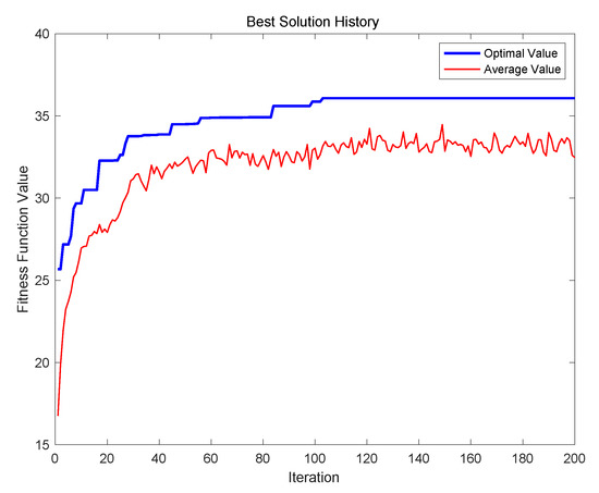
Figure 3.
Evolution results of PGA with 28 attractions.
The obtained satisfaction route is 0-2-27-22-24-21-20-26-23-16-19-18-17-13-11-6-0. The details of the results are illustrated in Table 3. The table contains seven items: recommended attraction, recommended arrival time, queuing time, time spent at the attraction, departure time from the attraction, walking time from this node to the next attraction, and the degree of satisfaction for selected attractions. The total walking time of the travel route is 92 min, the total queuing time is 372 min, the satisfaction of the tourists is 6.9, and the number of recommended attractions is 15.
Table 3.
Results of the satisfaction route with PGA (28 attractions).
Then, the evolution results of the improved APGA are illustrated in Figure 4. Here, we set the initial temperature to 90 and the cooling coefficient to 0.99. The best solution in the experiment can be found when the iteration is 156, and the value of fitness function is 36.0801. The result is the same as that of PGA, and the obtained satisfaction route is 0-2-27-22-24-21-20-26-23-16-19-18-17-13-11-6-0. The details of the results are illustrated in Table 4. As with Table 3, the table also contains seven items: recommended attraction, recommended arrival time, queuing time, playing time spent at the attraction, departure time from the attraction, walking time from this node to the next attraction, and the degree of satisfaction for selected attractions. The total walking time of the travel route is 92 min, the total queuing time is 372 min, the satisfaction of the tourists is 6.9, and the number of recommended attractions is also 15.
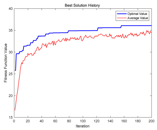
Figure 4.
Evolution results of APGA with 28 attractions.
Table 4.
Results of the satisfaction route with APGA (28 attractions).
By comparing the two results above, when there are 28 attractions, the best solution of the two different algorithms can be found in a short time. In addition, we tested the two algorithms 15 times. For the same example, Table 5 includes the test results using the PGA 15 times, and the second row is the optimal value of fitness function in the experiment corresponding to each test, and the third row is the obtained satisfaction route. Table 6 illustrates the test result acquired using the APGA 15 times. From Table 5 and Table 6, after being tested 15 times, the best solution was found once by using the PGA, while the best solution of 36.0801 was found twice by using the APGA. Table 7 illustrates the comparison results of the two different algorithms. The presented results are the best solution (Best), worst solution (Worst), average solution (Average), and the standard deviation (Std).
Table 5.
The results of 15 tests using the PGA (28 attractions).
Table 6.
The results of 15 tests using the APGA (28 attractions).
Table 7.
Comparison of different methods for solving time-varying theme park routing (TDTPRP) (28 attractions).
The test results indicate that both algorithms can be used to find the best solution within a short time when resolving the path of a theme park with 28 attractions. However, the APGA is superior to the PGA in terms of optimizing ability.
4.2. Randomly Generated Problem Instances
The results above demonstrate that both the PGA and the APGA mentioned in this paper can be used to find the best solution within a short time when resolving small and medium-sized theme park routing problems. Then, we expanded the test scale in the second test. We generated a theme park with one entrance and 60 attractions at random within a 2000 × 2000 test environment, as illustrated in Figure 5.
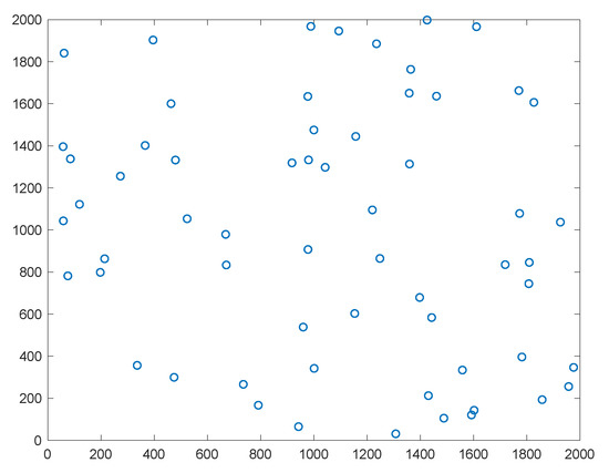
Figure 5.
Scatter plot
One of the points serves as the entrance (exit), and the remaining 60 points are regarded as the attractions. A visitor departing from the entrance of the theme park visits the attractions and then leaves the theme park. We randomly generated a simulated theme park environment and assumed that any two points are connected, and the distance between any two points is known. The time spent at the attraction, the queuing time, and the degree of satisfaction for each project are provided where the degree of satisfaction for the attractions are also generated from this interval [0, 1]. As with the previous experiment, we chose to use the same function to calculate the walking speed of the visitors.
The opening and the closing times are set as 09:00 and 17:00. The weights of the objectives are set to 0.2, 0.5, and 0.3, respectively, and conversion factors of utility ) are set to 1, 10, and 0.1, respectively. The population size is set to 200, and the maximum iteration is 200. The probabilities of the three genetic operators are generated randomly.
The evolution results of the PGA are illustrated in Figure 6, where the best solution in the experiment can be found when the iteration is 185, and the best value of fitness function is 34.0835.
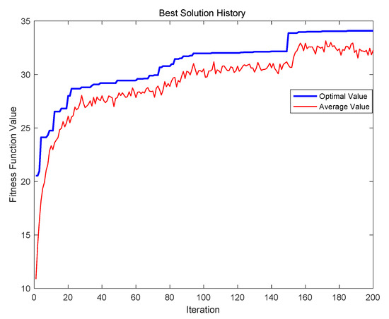
Figure 6.
Evolution results of PGA with 60 attractions.
The obtained satisfaction route is 0-6-18-26-7-10-30-9-44-8-21-0. Details on the results are illustrated in Table 8. The total walking time of the travel route is 61 min, the total queuing time is 282 min, the degree of satisfaction of the tourists is 8.53, and the number of recommended attractions is 10.
Table 8.
Results of the satisfaction route with PGA (60 attractions)
The evolution result of the improved APGA is illustrated in Figure 7, where the best solution in the experiment can be found when the iteration is 160, and the best value of fitness function is 34.1492. The obtained satisfaction route is 0-6-18-26-24-7-10-30-9-44-8-0. The details of the results are illustrated in Table 9. The total walking time of the travel route is 65 min, the total queuing time is 272 min, the satisfaction of tourists is 8.51, and the number of recommended attractions is 10.
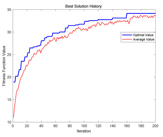
Figure 7.
Evolution results of APGA with 60 attractions.
Table 9.
Results of the satisfaction route with APGA (60 attractions)
If there are 28 attraction projects, the two different algorithms can be used to find the relative best solution within a short time successfully. However, when we increased the attractions to 60, the computation time of the PGA was longer, and it was inferior to the APGA in terms of optimizing ability. By comparing Figure 6 and Figure 7, the PGA was stuck in a locally optimal solution in the 185th generation, the best result was 34.0835, and it failed to reach the ideal result. By contrast, the APGA overcame the weakness of being stuck in local optimization and tended to be stable in the 160th generation. The best solution in this experiment was 34.1492.
Similarly, we ran the two algorithms 15 times in the test. Table 10 illustrates the test results acquired by using the PGA 15 times. Table 11 illustrates the test results acquired by the APGA. It can be concluded from the results that, if the PGA was used for the solution, the positive solution rate was 0, which means no best solution was found in the solution process using 15 tests. The best solution was found twice once the APGA was used, and Table 12 illustrates the comparison of the two algorithms.
Table 10.
The results of 15 tests using the PGA (60 attractions)
Table 11.
The results of 15 tests using the APGA (60 attractions)
Table 12.
Comparison of different methods for solving TDTPRP (60 attractions)
5. Discussion
In order to solve the problem of crowded queuing in large theme parks, improve visitor satisfaction, and reduce congestion, a time-dependent theme park routing problem (TDTPRP) was proposed to maximize the utility of the visitors and minimize queuing and walking times for selecting the optimal attractions under the framework of the traveling salesman problem (TSP), where walking time was treated as time-dependent and changed according to different time periods. This model can provide a more accurate plan and plan for a single decision. To solve the proposed model and verify the feasibility and the effectiveness of the model, we used a parthenogenetic algorithm and proposed an annealing parthenogenetic algorithm. In the experimental stage, we conducted two experiments; the experimental data were divided into real-world problems and randomly generated problems. First, we used the Tokyo Disney Sea with 28 attractions as the real-world problem to prove the effectiveness of the model and the algorithm. Second, to prove the stability of the model and the algorithm, we expanded the scale of the experiment and randomly generated an example of a theme park with 60 attractions within a 2000 × 2000 test environment. The results demonstrate that, when the experiment scale is small, the general parthenogenetic algorithm and the annealing parthenogenetic algorithm have the same excellent optimization ability, but the annealing parthenogenetic algorithm has better optimization ability than the general parthenogenetic algorithm when the data scale was expanded.
For future research, there is space for further improvements. For example, the walking time is dynamic, but to make it comparable to a realistic problem, the queuing time should also be constantly changing. Moreover, at present, some theme parks offer tickets to skip queues, some of which are free and some of which involve a fee. These factors could be considered in future research to continue to develop the model, and with the improvement of the model, the design of the algorithm should also continue to improve.
Author Contributions
Conceptualization, Z.Y.; methodology, Z.Y. and J.L.; software, Z.Y. and J.L.; validation, Z.Y., J.L. and L.L.; formal analysis, Z.Y.; investigation, Z.Y.; resources, Z.Y.; data curation, Z.Y.; writing-original draft preparation, Z.Y.; writing-review and editing, J.L. and L.L.; supervision, L.L. All authors have read and agreed to the published version of the manuscript.
Funding
This research received no external funding.
Conflicts of Interest
The authors declare no conflict of interest.
References
- Johns, N.; Gyimóthy, S. Mythologies of a theme park: An icon of modern family life. J. Vacat. Mark. 2002, 8, 320–331. [Google Scholar] [CrossRef]
- Kawamura, H.; Kurumatani, K.; Ohuchi, A. A study on coordination scheduling algorithm for theme park problem with multiagent. Inst. Electron. Inform. Commun. Eng. Tech. Rep. Artif. Intell. Knowl.-Based Process. 2003, 102, 25–30. [Google Scholar]
- Yasushi, Y.; Keiji, S. Comparison of Traversal Strategies in Theme Parks; Technical Report for IPSJ SIG Technical Reports (ICS-147); IPSJ: Tokyo, Japan, 2007; pp. 15–22. [Google Scholar]
- Kikuchi, S.; Onishi, K. A Sightseeing Route Guidance System using Java Applet. In Proceedings of the 54th National Convention IPSJ 1, Chiba, Japan, 12–14 March 1997; pp. 431–432. [Google Scholar]
- Matsuda, Y.; Nakamura, M.; Kang, D.; Miyagi, H. An Optimal Routing Problem for Sightseeing and its Solution. IEEJ Trans. Electron. Inf. Syst. 2004, 124, 1507–1514. [Google Scholar] [CrossRef][Green Version]
- Tsai, C.-Y.; Chung, S.-H. A personalized route recommendation service for theme parks using RFID information and tourist behavior. Decis. Support Syst. 2012, 52, 514–527. [Google Scholar] [CrossRef]
- Lee, C.-S.; Chang, Y.-C.; Wang, M.-H. Ontological recommendation multi-agent for Tainan City travel. Expert Syst. Appl. 2009, 36, 6740–6753. [Google Scholar] [CrossRef]
- Lim, K.H.; Chan, J.; Leckie, C.; Karunasekera, S. Personalized trip recommendation for tourists based on user interests, points of interest visit durations and visit recency. Knowl. Inf. Syst. 2017, 54, 375–406. [Google Scholar] [CrossRef]
- Mor, M.; Sagi, D. Computing touristic walking routes using geotagged photographs from Flickr. In Proceedings of the 14th International Conference on Location Based Services, Zurich, Switzerland, 15–17 January 2018. [Google Scholar]
- Gionis, A.; Lappas, T.; Pelechrinis, K.; Terzi, E. Customized tour recommendations in urban areas. In Proceedings of the 7th ACM International Conference on Web Search and Data Mining—WSDM ’14, New York, NY, USA, 24–28 February 2014; Association for Computing Machinery (ACM): New York, NY, USA, 2014; pp. 313–322. [Google Scholar]
- Sengupta, L.; Mariescu-Istodor, R.; Fränti, P. Planning Your Route: Where to Start? Comput. Brain Behav. 2018, 1, 252–265. [Google Scholar] [CrossRef]
- Niitsuma, H.; Arai, K.; Ohta, M. Efficient Constraints for Tour Recommendation. Inform. Process. Soc. Jpn. Database (TOD) 2016, 9, 34–45. [Google Scholar]
- Matsuda, Y.; Nakamura, M.; Kang, D.; Miyagi, H. An optimal routing problem for sightseeing with fuzzy time-varying weights. In Proceedings of the 2004 IEEE International Conference on Systems, Man and Cybernetics (IEEE Cat. No. 04CH37583), The Hague, The Netherlands, 10–13 October 2004; Volume 4. [Google Scholar]
- Little, J.D.C.; Murty, K.G.; Sweeney, D.W.; Karel, C. An Algorithm for the Traveling Salesman Problem. Oper. Res. 1963, 11, 972–989. [Google Scholar] [CrossRef]
- Laporte, G.; Martello, S. The selective travelling salesman problem. Discret. Appl. Math. 1990, 26, 193–207. [Google Scholar] [CrossRef]
- Feillet, D.; Dejax, P.; Gendreau, M. Traveling Salesman Problems with Profits. Transp. Sci. 2005, 39, 188–205. [Google Scholar] [CrossRef]
- Mak-Hau, V.; Thomadsen, T. Polyhedral combinatorics of the cardinality constrained quadratic knapsack problem and the quadratic selective travelling salesman problem. J. Comb. Optim. 2006, 11, 421–434. [Google Scholar] [CrossRef]
- Vansteenwegen, P.; Souffriau, W.; Van Oudheusden, D. The orienteering problem: A survey. Eur. J. Oper. Res. 2011, 209, 1–10. [Google Scholar] [CrossRef]
- Ergezer, H.; Leblebicioglu, K. Path Planning for UAVs for Maximum Information Collection. IEEE Trans. Aerosp. Electron. Syst. 2013, 49, 502–520. [Google Scholar] [CrossRef]
- Gendreau, M.; Laporte, G.; Semet, F. A tabu search heuristic for the undirected selective travelling salesman problem. Eur. J. Oper. Res. 1998, 106, 539–545. [Google Scholar] [CrossRef]
- Qin, H.; Lim, A.; Xu, D. The Selective Traveling Salesman Problem with Regular Working Time Windows; Springer Science and Business Media LLC: Berlin/Heidelberg, Germany, 2009; pp. 291–296. [Google Scholar]
- Ke, L.; Archetti, C.; Feng, Z. Ants can solve the team orienteering problem. Comput. Ind. Eng. 2008, 54, 648–665. [Google Scholar] [CrossRef]
- Bouzarth, E.L.; Forrester, R.J.; Hutson, K.R.; Isaac, R.; Midkiff, J.; Rivers, D.; Testa, L. A Comparison of Algorithms for Finding an Efficient Theme Park Tour. J. Appl. Math. 2018, 2018, 1–14. [Google Scholar] [CrossRef]
- Kanoh, H.; Ochiai, J. Solving Time-Dependent Traveling Salesman Problems Using Ant Colony Optimization Based on Predicted Traffic. In Advances in Soft Computing; Springer Science and Business Media LLC: Berlin/Heidelberg, Germany, 2012; Volume 151, pp. 25–32. [Google Scholar]
- Yanfeng, L.; Jun, L.; Da, Z. Dynasearch Algorithms for Solving Time Dependent Traveling Salesman Problem. J. SouthWest JiaoTong Univ. 2008, 43, 187–193. [Google Scholar]
- Maojun, L.; Tong, T. A parthenogenetic algorithm and analysis on its global convergence. Acta Autom. Sin. 1999, 25, 68–72. [Google Scholar]
- Gandomkar, M.; Vakilian, M.; Ehsan, M. A combination of genetic algorithm and simulated annealing for optimal DG allocation in distribution networks. In Proceedings of the Canada Conference on Electrical and Computer Engineering, Saskatoon, SK, Canada, 1–4 May 2005. [Google Scholar] [CrossRef]
- Tian, Q.C.; Pan, Q.; Wang, F.; Zhang, H.C. Research on Learning Algorithm of BP Neural Network Based on the Metropolis Criterion. Tech. Autom. Appl. 2003, 5, 15–17. [Google Scholar]
- Liu, L.; Olszewski, P.; Goh, P.-C. Combined Simulated Annealing and Genetic Algorithm Approach to Bus Network Design. In International Conference on Transport Systems Telematics; Springer Science and Business Media LLC: Berlin/Heidelberg, Germany, 2010; pp. 335–346. [Google Scholar]
- Suppapitnarm, A.; Seffen, K.A.; Parks, G.T.; Clarkson, P.J. A simulated annealing algorithm for multiobjective optimization. Eng. Optim. 2000, 33, 59–85. [Google Scholar] [CrossRef]
Publisher’s Note: MDPI stays neutral with regard to jurisdictional claims in published maps and institutional affiliations. |
© 2020 by the authors. Licensee MDPI, Basel, Switzerland. This article is an open access article distributed under the terms and conditions of the Creative Commons Attribution (CC BY) license (http://creativecommons.org/licenses/by/4.0/).