Abstract
The semi-nonparametric (SNP) modeling of the return distribution has been proved to be a flexible and accurate methodology for portfolio risk management that allows two-step estimation of the dynamic conditional correlation (DCC) matrix. For this SNP-DCC model, we propose a stepwise procedure to compute pairwise conditional correlations under bivariate marginal SNP distributions, overcoming the curse of dimensionality. The procedure is compared to the assumption of dynamic equicorrelation (DECO), which is a parsimonious model when correlations among the assets are not significantly different but requires joint estimation of the multivariate SNP model. The risk assessment of both methodologies is tested for a portfolio of cryptocurrencies by implementing backtesting techniques and for different risk measures: value-at-risk, expected shortfall and median shortfall. The results support our proposal showing that the SNP-DCC model has better performance for lower confidence levels than the SNP-DECO model and is more appropriate for portfolio diversification purposes.
1. Introduction
The analysis of portfolio risk requires statistical models and techniques that accurately capture the (time-varying) dependence between prices or returns of individual assets and account for salient characteristics of the individual (marginal) distributions. For this purpose, in the last decades, there is abundant literature devoted to extending the risk modeling to the multivariate context. One of the most successful approaches are the multivariate GARCH-family models that parameterize the variance–covariance matrix through different specifications, e.g., the Vech model [1], the factor GARCH [2], the constant conditional correlation (CCC) model [3], the BEKK model [4], the dynamic conditional correlation (DCC) model [5] or the dynamic equicorrelation model (DECO) [6], among others—see [7], for a comprehensive survey. All of these models, parsimoniously feature the dependence structure, thus (partially) tackling the “curse of dimensionality”, but their extension beyond the normality assumption is far from trivial.
Different solutions have been provided to model the multivariate non-Gaussian distribution of asset returns. On the one hand, [8] showed that under correct specification of the conditional mean-variance model, maximum likelihood (ML) estimation under the Gaussian distribution provides consistent estimates even when normality is violated, which is the basis of the quasi ML (QML) estimation. On the other hand, many non-Gaussian distributions straightforwardly admit a multivariate GARCH-family structure, particularly the class of elliptical distributions [9]. However, these extensions are developed at the cost of losing the consistency of the two-step estimation (i.e., with a higher computational burden), which is feasible under Gaussianity [10], and their capacity to account for tail dependence is rather limited.
Within the methods to define multivariate distributions [11], a particularly appealing solution to all these problems is the use of copulas, which allow deriving a multivariate distribution with a dependence measure from a group of arbitrary marginal distributions, in virtue of the Sklar’s theorem—see, e.g., [12]. However, the moment computation of the applications that involve integration (e.g., providing risk measures) becomes analytically intractable and requires numerical algorithms [13].
Another interesting approach is the semi-nonparametric (SNP) extension of the multivariate Gaussian through Gram–Charlier (GC) series. As a matter of fact, GC series have been proved, under regularity conditions, to be a valid asymptotic expansion of any distribution, see [14] or [15]. A multivariate extension of the GC distribution was explored by [16,17,18]. In particular, the two latter showed the utility of these distributions to capture the distribution of portfolios of financial returns. Since then, alternative versions have been proposed to tackle different problems: positivity [19], two-step estimation [20], approximation properties [21], generalizations to other distributions [22], method of moments estimation [23], time-varying conditional moments [24], specifications in vector notation [25], or risk forecasting [26]. These models not only preserve the asymptotic approximation property, but also are very tractable from both the theoretical and empirical viewpoint. Although the curse of dimensionality is a little more serious than in other models, it can be smoothed through the implementation of two-step or recursive estimation methods. Furthermore, this approach naturally admits the incorporation of multivariate GARCH-family models as CCC, DCC, or DECO.
This research is focused on assessing the performance of the multivariate positive GC distribution [27], that implies a symmetric distribution being positive in the whole domain for capturing the risk of highly volatile assets. To this end, we analyze portfolios of cryptocurrencies, which are modeled as AR-GJR-GARCH [28] (i.e., considering asymmetric conditional variances) and a covariance structure consistent to either DCC or DECO. The former is estimated through a simplifying method based on the estimation of bivariate models and the latter is jointly estimated but assuming equal correlation among the crypto assets. The comparison of both methods sheds light on the gains of simplifying the estimation method or the correlation dynamics when dealing with the computational burden of multivariate SNP modeling.
The performance will be evaluated in terms of three alternative risk measures: value-at-risk (VaR), median shortfall (MS), and expected shortfall (ES). Each of them has supporters and opponents, but VaR and ES have been the most used in the financial industry for the last years. In addition to these traditional measures, we consider MS, which can be easily computed as a higher level of VaR and, to the best of our knowledge, is barely used related to cryptocurrencies [29], despite being a more robust measure in the presence of extreme events.
In order to assess the model validation, we consider backtesting techniques applying the conditional coverage (CC) test [30] and dynamic quantile (DQ) test [31] for both VaR and MS. For ES we apply recently developed tests for backtesting: multinomial test [32] and ES regression test [33], the latter being the first ES test that only requires ES forecasts as input parameters regardless of VaR.
Our findings indicate that SNP-DCC and SNP-DECO show small differences between both methodologies in all portfolios selected. The results support our new proposal of implementing SNP-DCC as an acceptable alternative to model larger portfolios tackling the curse of dimensionality considering a two-step method. In general, there is hardly any difference between 97.5%-MS and 99%-VaR, but for 97.5%-VaR the best results are for SNP-DCC model, especially with portfolios less volatile and with higher correlations. On the other hand, for the far-end tail, the results are slightly better for the SNP-DECO model. For ES, the empirical application shows excellent results for both models being slightly better for portfolios with higher volatile and less correlated assets.
The remaining of the article is structured as follows: Section 2 revises the multivariate GC model specified with either DCC or DECO structures and portfolio risk performance measures. Section 3 introduces cryptocurrencies and performs an application of the models described in Section 2 for a three-variate portfolio on three salient crypto assets: Bitcoin, Litecoin, and Ripple. Finally, Section 4 summaries what we have learned from the two methods for computing portfolio risk with GC distributions.
2. The Model
2.1. Multivariate Gram–Charlier Model
A multivariate GC expansion of a given pdf , , can be expressed as the following infinite series of the derivatives of order of the multivariate normal pdf, , as shown in Equations (1)–(5)—see [34]:
where, for convenient purposes, we consider the standard multivariate normal pdf—i.e., vector has 0 mean and (identity or order n) matrix,
and
being the joint cumulants of the vector , which are related to the derivatives of the natural logarithm of the characteristic function :
where
the symbol representing the scalar product of two vectors and
This is a nice definition, but, unfortunately, for empirical purposes becomes intractable unless small (finite) orders for the expansions and the vector dimension n are considered. For this reason, Ref. [20] provided a feasible expression for the multivariate Gram–Charlier density (referred to as SNP density), which is directly formulated in terms of the product of n independent (univariate) marginal Gram–Charlier expansions, as given in Equations (6)–(8):
where ϕ and is a m-order Gram–Charlier expansion (without loss of generalization we consider the same m for all n dimensions) expressed in terms of Hermite polynomials, i.e.,
In order to solve potential positivity problems of the truncated GC series, which is particularly important when applying backtesting techniques, positive transformations can be directly implemented. For instance, the transformation provided by [27] may be considered by replacing Equation (7) by Equation (9):
This extension of the multivariate GC density is a well-defined density although its statistical properties are slightly different to the original multivariate GC distribution (see [19]).
The Hermite polynomials satisfy well-known orthogonality properties—Equations (10) and (11),
which are the basis of being a density when expansions are truncated at a finite n. Furthermore, the first six Hermite polynomials are, , , , ,, The higher-order parameters account for extreme values and jumps at the distribution tails, and, if necessary, make the semi-nonparametric Gram–Charlier expansion approximate any “regular” pdf.
In addition, the ability of the (multivariate) Gram–Charlier family to adopt a wide variety of shapes with a flexible number of parameters, including fat tails with non-monotonic decay, this distribution presents three interesting properties:
(i) Marginals are also Gram–Charlier distributed, the univariate marginals being described in Equation (12).
(ii) Both linear transformations and linear combinations are also Gram–Charlier distributed [35]. As a consequence, the pdf of the vector can be expressed as in Equation (13).
Note that the (positive definite) variance and covariance matrix can be expressed as where is a diagonal matrix containing conditional volatilities and a correlation matrix that can be decomposed as (e.g., spectral decomposition).
Furthermore, if then, is a univariate Gram–Charlier with conditional mean and conditional variance .
(iii) The Log-likelihood of conditional mean-variance and the rest of the distribution is separable, and thus the two-step estimation procedures may be implemented—see [20] for further details. Particularly, in the first step conditional mean and variance can be estimated by quasi maximum likelihood (QML) and in the second step the rest of the parameters of the Gram–Charlier density, including the conditional correlations, should be jointly estimated.
2.2. The Dynamic Conditional Correlation Model
The property (ii) in the above section allows the consideration of the dynamic nature of conditional variance and covariance matrix by alternative multivariate GARCH models. In this paper we focus on the SNP-DCC and the SNP-DECO models, for returns filtered through standard ARMA models for conditional mean (particularly we use an AR(1)) and a version of the GJR model [28] for conditional variance—see [36] or [37]. This model allows asymmetric responses of conditional variances to negative and positive shocks. The asymmetric response of conditional correlation might also be included, but the implementation of the AGDCC [38] model with SNP distributions is left for further research. All in all, the final model can be parameterized as in Equations (14)–(21)—note that the correlation matrix of DCC and DECO are represented by Equations (19) and (20), respectively:
where , , , and ; ; is the unconditional correlation matrix; is a vector of ones; A, B, and ii′ − A − B positive definite matrices; (a diagonal matrix with the same diagonal as ) and the Hadamard product of two identically sized matrices (computed by element-by-element multiplication). For the DECO model, is an identity matrix of order one, is a matrix of ones and is set equal to the average pairwise DCC correlations as in Equation (20), where is the ith row and jth column element of .
These models were originally defined for the Gaussian distribution. In this research, we assume a Gram–Charlier conditioned on the information set , as stated in Equation (15). This involves a non-trivial evaluation of the polynomial terms in Equation (9) on , which for the bivariate DCC model results in Equation (22)—see [20]:
where and .
Likewise, for the DECO model, may be written as in Equation (23)—see [22]:
where .
The DECO model greatly simplifies the estimation, but at the cost of imposing the same correlation among all variables. In addition, the DCC considers a richer time-varying correlation structure but is more dependent on the “curse of dimensionality” of multivariate modeling. As an intermediate solution, we propose a procedure that implements the DCC model estimation by exploiting the properties of the Gram–Charlier and, particularly, the independent estimation of the conditional correlation parameters in the bivariate Gram–Charlier marginal densities defined in Equation (24). It is noteworthy that if marginals are defined in terms of the bivariate marginal distribution is dependent on the dimension n of the original vector for which the marginal is computed, e.g., the bivariate distribution becomes the Equation (24)—see the proof in Appendix A:
For the returns series of the portfolio defined in Equation (26) and such that = 1, 2, …, n and , our procedure can be described in the following four stages.
Stage 1: Independent estimation of portfolio conditional mean and variance for each univariate pdfs (QML).
Stage 2: Using the standardized variables filtered through the estimates obtained in stage 1, conditional correlations for each pairwise variables are estimated under a bivariate Gram–Charlier density for DCC and with joint estimation for DECO (since the latter requires imposing the same structure for all dimensions).
Stage 3: The portfolio’s Gram–Charlier distribution is estimated for the univariate series standardized by the forecasted portfolio mean-variance model according to the estimates in stages 1 and 2.
Stage 4: Given the quantiles of the portfolio distribution (Stage 3) and the estimates for its mean-variance model (stages 1 and 2) risk assessment in terms of value at risk (VaR) and expected shortfall (ES) of the Gram–Charlier under DECO and DCC is tested.
2.3. Risk Performance Model
Risk forecasting methods provide an excellent approach to assess the level of risk for portfolios on the basis of the accurate estimation of both the correlation matrix and distribution tails. To compare the best model validation, we have chosen three major risk measures: value-at-risk (VaR), expected shortfall (ES), and median shortfall (MS).
VaR is the best-known measure in the risk management industry. It started employing as capital adequacy measures for banks and it is widely used in the global financial industry [39]. It can be defined as the maximum potential loss for the portfolio (P) return with a confidence level for a time horizon and it is represented in Equation (25)
where and are the one-step ahead forecasted conditional mean and conditional standard deviation for the portfolio in Equation (26), and the estimated α-quantile of the assumed (n-asset) conditional portfolio distribution.
Given the weight of the return of every, the portfolio mean and variance can be straightforwardly obtained as in Equations (27) and (28), respectively,
where and are the conditional mean and standard deviation of asset i, and is the conditional correlation of every (i and j) asset pairwise.
The portfolio quantile , where depicts the cumulative distribution function (cdf) that, for the case of the GC distribution, can be computed from Equation (29),
or, alternatively, for the positive version in Equations (6) and (9)—see [27], as in Equation (30),
It is noteworthy that these quantiles require the estimation of portfolio density parameters (). Alternatively, the quantiles can be directly obtained evaluating the standardized GC density in Equation (6) (i.e., with identity variance and covariance matrix) on the transformed values according to Equations (22) and (23), since these values incorporate the information of the conditional variance and covariance structure.
However, one of the major drawbacks in VaR computation is using only a quantile, disregarding the rest of the values in the tail of the distribution and thus being more sensitive to extreme values. For the purpose of robustness, we consider the MS, which is the median of the tail given a significance level . The performance of this latter measure has been studied in other areas [40,41], but to the best of our knowledge, it is not commonly used with cryptocurrencies. It may be directly computed from VaR as in Equation (31),
provided that the loss exceeds the VaR at level α [42] and it is based on the equivalence with VaR where the 99%-MS and 97.5%-MS are estimated as 99.5%-VaR and 98.75%-VaR, respectively.
Finally, the third risk measure is the ES, defined in Equation (32), which is more sensitive to events in the tail end of a distribution beyond VaR,
For convenience, an approximation to ES can be obtained by averaging N quantiles with different confidence levels [43], e.g., for N = 8, in Equation (33)
Model performance is assessed through backtesting techniques, which evaluate any forecasted risk measure through the out-of-sample (backtesting) period on the basis of the information of a (usually rolling) in-sample window. This method seems appropriate for stationary series, and provided that the moments of the distribution exist, condition that is satisfied for the SNP modeling. Appropriate tests for backtesting risk measures are also selected. Particularly, for VaR and MS backtesting, the CC test is implemented where the null hypothesis is the correct model specification, and the exceptions satisfy the unconditional coverage and independence test. Results are complemented by the DQ test (with 4 lags) and the actual over expected (AE) ratio, the latter comparing the number of observed over expected exceptions, i.e., the closer to one the better the model.
Regarding ES, we apply the ES regression [33], ESR hereafter, a brand-new backtesting ES forecast and, to the best of our knowledge, barely used in cryptos [29]. We propose one of its specifications which consists in testing one-sided (such as most of the VaR backtest) beside two-sided alternatives: Intercept ESR which is the first test for ES stand-alone and consists of a regression framework for the forecast errors on an intercept term in the ES regression equation. It only requires ES forecasts as input parameters regardless of VaR, fixing the slope parameter to one in the regression and only estimating the intercept term.
3. Empirical Application
3.1. Cryptocurrencies
The fast-growing cryptocurrency industry emerged just over a decade ago, in 2009 since the inception of the Bitcoin in the market [44]. Cryptocurrencies exhibit specific features which make it different from other assets [45,46]. They have a decentralized structure where regulatory or financial institutions are replaced by algorithms which check cryptocurrencies behavior guaranteeing an effective performance. Nowadays there are more than five thousand cryptocurrencies where the eighty-eight per cent out of the total market capitalization is covered by only ten of them, exceeding two hundred and forty-four billion dollars where Bitcoin represents over sixty-five per cent (coinmarketcap.com). Even though their origin was to be able to make simple and fast payments on a peer-to-peer process based on blockchain technology, they have become an appealing asset to invest or speculate due to their high volatility.
This new disruptive technology is deeming increasing interest being carefully studied by regulators, academics, policymakers, governments, and institutions. Not only about their most differentiating characteristics [47,48,49,50] but also for the analysis of volatility models [45,51,52,53,54,55] and risk forecasts [36]. Their behavior for hedging has been studied in portfolios with other kinds of assets [56,57], or with others cryptos [29,58,59,60]. Our application fits in this latter framework, since GC models are applied to a portfolio with the three best known and most representative crypto assets: Bitcoin, Litecoin, and Ripple. A short comment on each one can be find in Appendix B.
3.2. Data Description and Analysis
Cryptos are 24/7 trading and we consider the closing time at midnight (UTC time). Daily prices () ranged from 4 August 2013 to 6 March 2020 (T = 2407 observations downloaded from www.coinmarketcap.com on 5 June 2020) computed daily percentage log-returns in Equation (34).
In our application, four different weighted portfolios are formed from Bitcoin (BTC), Litecoin (LTC), and Ripple (XRP). The first portfolio (P-I) is an equally weighted portfolio; the second portfolio (P-II) is a portfolio of 25% BTC, 25% LTC, and 50% XRP; the third portfolio (P-III) is a combination of 25% BTC, 50% LTC, and 25% XRP; and the forth portfolio (P-IV) is a portfolio of 50% BTC, 25% LTC, and 25% XRP. Table 1 shows the descriptive statistics for the individual cryptos and its portfolios and Figure 1 illustrates the evolution of the cryptocurrency series in levels and log-returns. It is noteworthy the episodes of sharp increase in the prices (particularly in 2018) and the clustering and presence of extreme values in volatility dynamics. However, the series seem to exhibit the typical regularities of most financial daily returns.

Table 1.
Descriptive Statistics for Cryptocurrency Returns.
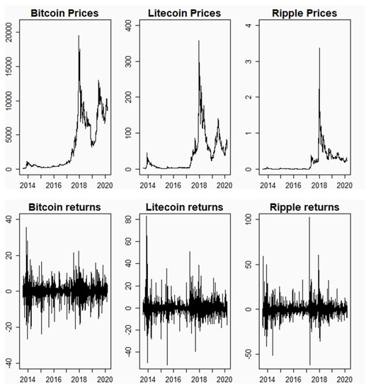
Figure 1.
Cryptocurrency prices and returns for Bitcoin, Litecoin, and Ripple series. Daily prices from 4 August 2013 to 6 March 2020 (2407 observations).
Regarding individual cryptocurrency leptokurtosis, Litecoin and Ripple both exhibit excess kurtosis more than three times that of the Bitcoin. All the cryptocurrency distributions are positively skewed except for Bitcoin, which is negatively skewed. Moreover, Bitcoin is the less volatile asset (daily standard deviation of 4.21) in comparison to the Litecoin and Ripple in the analyzed period.
It is noteworthy to mention that constructed portfolios present similar characteristics but slightly smoother than cryptos, where leptokurtosis is prominent but less variable among them (excess kurtosis ranges from 10.493 to 14.161). All portfolio distributions are positively skewed, where skewness values are between 0.193 (P-IV) and 0.885 (P-II). Whereas daily portfolio volatility ranges between 4.445 and 5.102.
Table 2 displays the results of the unconditional correlation matrix for all returns sample in order to provide preliminary information about the correlation before analyzing the performance of conditional correlations.
Table 2.
Unconditional Correlation Matrix for Cryptocurrency Returns.
The unconditional correlation coefficients show the strengths of the linear relationship among cryptos. All the correlations are positive, the highest value being that for Bitcoin–Litecoin (0.665) and values for Bitcoin–Ripple, and Litecoin–Ripple exhibiting similar moderate correlation close to 0.40.
The backtesting of risk measures (VaR, MS, and ES) is performed by employing a constant-sized in-sample period of 1906 observations and an out-of-sample period of N = 500 days. For the sake of comparison, we consider the four portfolios previously detailed and the SNP-DCC model (Panel A) and SNP-DECO model (Panel B).
3.2.1. Value at Risk and Median Shortfall
Backtesting results for VaR are displayed in Table 3, p-value in parenthesis, for 99%-VaR and 97.5% with two different tests and one ratio, in order to obtain more information about the results: (1) conditional coverage test (CC), which test jointly unconditional coverage and independence test, (2) dynamic quantile (DQ hereafter) test with 4 lags, proposed by [31], and (3) the actual over expected (AE) ratio comparing the number of observed over expected exceptions.
Table 3.
VaR Backtesting for semi-nonparametric (SNP) DCC and DECO Models.
We provide two analysis depending on the number of exceptions and the results for the VaR tests, both for 99%-VaR and 97.5%-VaR, the standard measures for Basel II. Focusing on the former, the obtained exceptions, regardless the level of confidence of VaR, of the two models in all portfolios, are always higher than the expected exceptions except for 97.5%-VaR for DECO in Portfolio II. The comparison between expected and realized exceptions is displayed in Table 2, where the AE ratio compares the number of observed over-expected exceptions (the closer to one the better the model). This ratio is higher than one for all the models, except to 97.5%-VaR for DECO in Portfolio II (0.880). Following this line, the best models with the same number of expected and observed expectations are for 97.5%-VaR for DECO for Portfolio I and IV (AE ratio 1.040). Table 2 shows that 97.5%-VaR for DECO models provide fewer exceptions than DCC models and for 99%-VaR the AE ratio is similar.
Regarding the VaR tests, we provide CC and DQ statistics for different confidence levels. The results show that the performance for both models (DCC and DECO) for 99%-VaR and 97.5%-VaR are rather similar. That supports our proposal to implement DCC model estimation as the independent estimation of the conditional correlation parameters with the bivariate Gram–Charlier marginal densities where the results for both models should be comparable. For 99%-VaR, there is hardly any difference in the result for both models, however for a smaller quantile, as in the case 97.5%-VaR, DCC is being slightly better except for Portfolio II with a higher weighting for Ripple, the crypto with a greater volatility than the other two and with the lower correlation among them. For this confidence level, Portfolio IV shows the best result that corresponds to a higher weight of Bitcoin (50%), the less volatile crypto and portfolio in our application.
The null hypothesis represents the correct model specification for both tests and it is rejected for DCC and DECO models for Portfolio I and IV (99%-VaR). In regard to DQ test, it is also rejected even when p-value in the CC test is close to 0.06 of the significance level.
Figure 2 shows the four portfolio returns and the estimated 99%-VaR and 97.5%-VaR either DCC (Panel A) or DECO (Panel B).
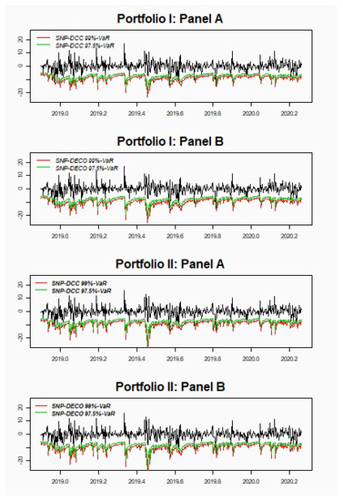
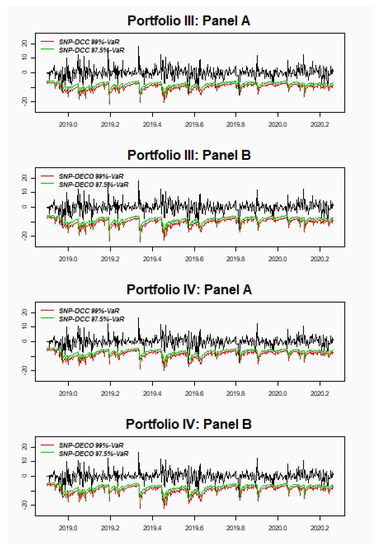
Figure 2.
Portfolio returns (black line) compared to 99% Value at Risk (VaR) (red line) and 97.5%-VaR (green line) for the four portfolios with both dynamic conditional correlation (DCC) and dynamic equicorrelation (DECO) models. Portfolio I corresponds to equally weighted portfolio; Portfolio II is 25% Bitcoin (BTC), 25% Litecoin (LTC), and 50% Ripple (XRP); Portfolio III is a combination of 25% BTC, 50% LTC, and 25% XRP; and Portfolio IV is 50% BTC, 25% LTC, and 25% XRP. Panel A (B) displays the DCC (DECO) model for every portfolio.
Once again, similar results are obtained in terms of the MS risk measure, since it is computed as a VaR but with a higher confidence level. The performance of the DCC and DECO models in terms of 99%-MS and 97.5%-MS is displayed in Table 4 and depicted in Figure 2. The null hypothesis for the CC test is not rejected in any case, except for Portfolio I for 99%-MS for DCC-SNP model. Each pair for 97.5%-MS of Portfolio I, II and IV have the same good results. In the case of 99%-MS, Panel B (DECO model) for all the portfolios seem to have better results than Panel A where a stronger weight of LTC in the portfolio fits better to 99%-MS. For 99%-MS the best models are for the SNP-DECO, although for 97.5%-MS the results are more homogeneous between models. The DQ test has similar results to the CC test although it is also rejected even when the p-value in the CC test is close to 0.11.
Table 4.
Median shortfall Backtesting for semi-nonparametric (SNP) DCC and DECO Models.
Depending on the different level of confidence in VaR, including MS, it seems that there is a slight change in the results from DECO to DCC. For 99%-MS (i.e., 99.5%-VaR) DECO model is slightly better to DCC. For the following two confidence levels, 99%-VaR and 97.5%-MS (98.75%-VaR) the results for each pair of models are rather similar whilst for 97.5%-VaR the best results are for DCC.
An illustration of the backtesting performance between 99%-MS and 97.5%-MS for the four portfolios with both DCC and DECO is presented in Figure 3.
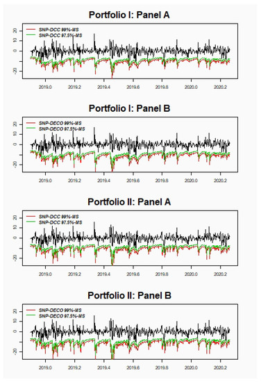
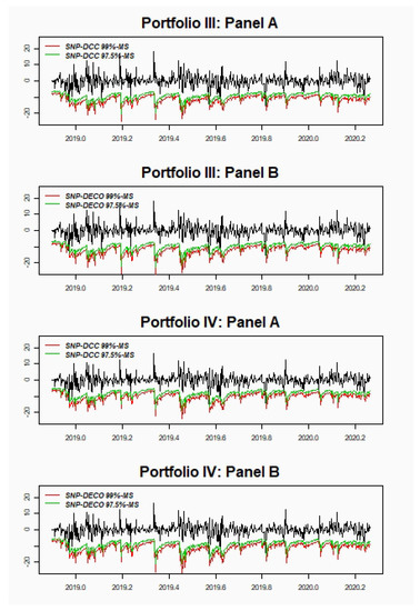
Figure 3.
Portfolio returns (black line) compared to 99% median shortfall (MS) (red line) and 97.5%-MS (green line) for four portfolios with both dynamic conditional correlation (DCC) and dynamic equicorrelation (DECO). Portfolio I corresponds to equally weighted portfolio; Portfolio II is 25% Bitcoin (BTC), 25% Litecoin (LTC), and 50% Ripple (XRP); Portfolio III is a combination of 25% BTC, 50% LTC, and 25% XRP; and Portfolio IV is 50% BTC, 25% LTC, and 25% XRP. Panel A (B) displays the SNP (DECO) model for every portfolio.
3.2.2. Expected Shortfall
Following the Basel Committee on Banking Supervision (BCBS), we compute 97.5%-ES as a comparable risk measure to 99%-VaR, but probably more accurate and consistent with portfolio diversification (since ES satisfies the subadditivity property, unlike VaR). However, ES is not elicitable being ES more burdensome than backtesting VaR. For this reason, Basel Committee (2016) propose to estimate ES but backtesting only VaR [61]. However, there is still a debate on the appropriateness of ES vs. VaR and the dependence of quantile-based risk measures on the underlying distribution (see, e.g., [62,63]). Since two alternatives for computing ES have been shown, for comparison purposes, two tests have also been considered, Intercept ES test and the Multinomial test [32]. The results are presented in Table 5. The Intercept ESR backtest allow us to compare one-sided with two-sided alternatives. This strict ES is pioneering, according to their authors [33], since it only requires ES forecast regardless of VaR, showing one-sided and two-sided alternatives in the final results. This is the reason why we have decided to select this test following the line of the Basel Committee for VaR (one-sided test) and compare with the two-sided version. For both sided alternatives, the null hypothesis of correct model specification is not rejected in any of both models regardless the portfolio weight. For one-sided, the best results are for the DECO model, as well as two-sided, particularly for Portfolios II and III where BTC has less weight than the other portfolios.
Table 5.
Expected Shortfall Backtesting for semi-nonparametric (SNP) DCC and DECO Models.
The multinomial test considers the numbers of exceptions in each day for the different levels of VaR, considering a maximum of eight (N = 8) of exceptions, setting a vector which follows a multinomial distribution where Pearson and Nass tests are used to assess the model performance—see also [32] for a related backtesting ES technique. Critical values (considering a backtesting period of 500) for both tests for N = 8 are 15.51 and 12.77, respectively. It should be pointed out that the approximation ES is an average of VaRs and the behavior in comparison to ESR-Intercept is slightly different, being more accurate the latter. According to Pearson and Nass test, Portfolio II and III, those with the highest volatility, are not rejected, especially Portfolio II where DCC seems to be preferable than DECO. The comparison for 97.5%-ES for both models and the four portfolios are also presented in Figure 4.
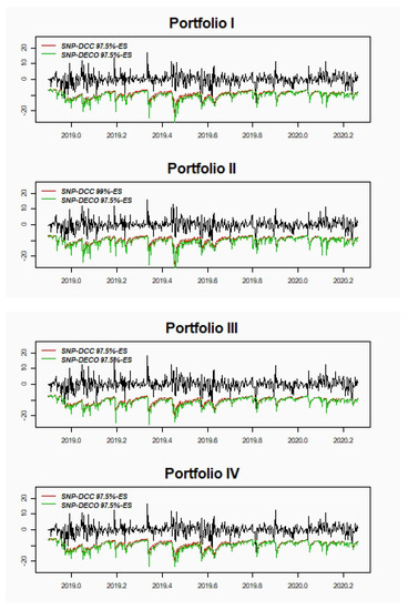
Figure 4.
Portfolio returns (black line) compared to 97.5% expected shortfall (ES) for four portfolios with both DCC (red line) and DECO (green line). Portfolio I corresponds to equally weighted portfolio; Portfolio II is 25% Bitcoin (BTC), 25% Litecoin (LTC), and 50% Ripple (XRP); Portfolio III is 25% BTC, 50% LTC, and 25% XRP; and Portfolio IV is 50% BTC, 25% LTC, and 25% XRP.
3.2.3. Summary of Results and Discussion
The empirical evidence shows that the DCC procedure is a tractable method to estimate SNP portfolio densities by decomposing the multivariate distribution in bivariate densities. The procedure seems to provide similar performance than the DECO model, and even exhibits the best result for the smallest confidence level (97.5%-VaR) for all the portfolios except portfolio II, which exhibits the highest volatility and assigns a higher weight to Ripple, the crypto with smaller correlation to the other assets. However, for higher confidence levels, such as 97.5%-MS (98.75%-VaR) and 99%-VaR, the results are rather similar and for the highest level, 99%-MS (99.5%-VaR), it seems SNP-DECO provides better results. Our findings appear to show that SNP-DCC works better with smaller confidence level whilst DECO is better for the far end of the tail.
In particular, for the CC test DCC seems to underestimate 99%-VaR for portfolios I-IV (less volatile) but with portfolios II and III (exhibiting higher volatility) it presents better assessment. On the other hand, considering a significance level of 5%, the null hypothesis is not rejected for both MS (97.5%-MS and 99%-MS) showing the same results for all portfolios for 97.5%-MS for both models. In the case of the 97.5%-ES, the null hypothesis is not rejected for any portfolio and model, presenting slightly better results for portfolio II and III which are the highest volatile portfolios with the lower correlation with BTC.
To provide more information about the impact of every asset on portfolio risk we present an example of the incremental VaR and ES when increasing the investment position on every crypto. Table 6 overviews the sum of each individual VaR, known as Undiversified VaR. The first column displays the 99%-VaR and 97.5%-VaR corresponding to a $300,000 investment equally distributed among the three cryptocurrencies. For the rest of the columns, it is considered a $100,000 increase, in Ripple (portfolio II), Litecoin (portfolio III) and Bitcoin (portfolio IV). The risk differences between portfolios II, III, and IV, and portfolio I is considered as incremental VaR [64,65,66,67,68] since they measure the effect on portfolio VaR from increasing the investment position in every asset.
Table 6.
Undiversified Portfolio VaR.
Since assets are not perfectly correlated, the portfolio VaR is lower than the sum of their components, and thus the correct estimation of the conditional correlation is crucial for diversification purposes. Furthermore, in this paper we have shown that the estimation of conditional correlation is dependent on the model specification, the SNP being a flexible and accurate approach that can be estimated with ease by means of either “recursive” DCC or “restrictive” DECO estimation. The effect of these two models on portfolio (diversified) VaR and ES is illustrated in Table 7 and Table 8, respectively, (Panel A and B include the risk measures for DCC and DECO, respectively). As in the case of undiversified VaR, Portfolio I assumes an equally-weighted $300,000 investment and portfolios II, III, and IV we increase in $100,000 the investment of Ripple, Litecoin, and Bitcoin, respectively. In Table 7 both 99%-VaR and 97.5%-VaR is computed and the incremental VaRs with respect to the Portfolio I are displayed in parentheses. It is noteworthy that, in all cases, DECO model implies higher VaR than DCC, the latter being the best (more flexible) option for diversification and hedging purposes. Even more, Litecoin and Ripple represent higher risk sources than Bitcoin, which is consistent with our finding of the best performance of the SNP-DCC model to capture the risk of portfolios that overweight these cryptocurrencies.
Table 7.
Portfolio Incremental VaR for the SNP-DCC and SNP-DECO Models.
Table 8.
Portfolio Incremental Expected Shortfall for the SNP-DCC and SNP-DECO Models.
Table 8 shows the Incremental ES computed from both direct ES and the approximation ES—see Equation (33), the latter systematically undervaluing the risk figures. Regardless of the type of ES, Panel A exhibits lower risk measures than Panel B, which means that DECO models imply more capital requirements due to its less flexible correlation structure. The overall behavior among all the portfolios is in line with VaR and thus the stepwise procedure for estimating SNP-DCC seems to provide better results for diversification purposes.
4. Conclusions
In the last decades, there have been proposed a vast literature on methodologies and models to improve portfolio risk measures. This paper focuses on the multivariate SNP modeling of the return distribution based on the GC series approximation, which has been scarcely used despite its advantages in terms of flexibility and accuracy. However, the curse of dimensionality is even more severe in this framework, which calls for solutions that make portfolio estimation tractable. Based on the properties of the SNP distribution we propose a very simple and consistent method of estimation that consists of estimating the DCC model on bivariate marginal SNP distributions and plugging these dynamic correlations on the univariate portfolio SNP distribution. We argue that this method is feasible even for large portfolios although at the cost of an increase in the number of correlations/distributions to estimate. However, such a procedure is even more appealing than the DECO model, a straightforward alternative, since DECO requires a joint estimation of the SNP distribution, which is very computationally demanding even when it considers a very naive correlation structure.
The performance of both the SNP-DCC (stepwise procedure) and the (jointly estimating) SNP-DECO are tested for several portfolios of major cryptocurrencies including Bitcoin, Litecoin, and Ripple. The model incorporates also a multivariate AR-GJR-GARCH structure and positivity transformations of the SNP density. Performance is compared through backtesting procedures for different risk measures 97.5% and 99% VaR and MS and 97.5%-ES. The implemented tests find small differences between both methodologies, supporting our proposal to implement the SNP-DCC model estimation with the bivariate Gram–Charlier marginal densities. Furthermore, the SNP-DCC model seems to provide lower risk portfolio measures since it exploits the more flexible correlation structure than the SNP-DECO, thus being preferable for diversification and hedging.
All of this suggests that the stepwise procedure for estimating SNP-DCC seems to be a very simple and accurate method for risk management, particularly useful for large portfolios where assets feature different characteristics in terms of volatility and correlation (i.e., more diversified) and when risk measures are computed at 97.5% confidence level.
Author Contributions
Conceptualization, I.J., A.M.-V., T.-M.Ñ. and J.P.; methodology, I.J., A.M.-V., T.-M.Ñ. and J.P.; software, I.J., A.M.-V., T.-M.Ñ. and J.P.; validation, I.J., A.M.-V., T.-M.Ñ. and J.P.; formal analysis, I.J., A.M.-V., T.-M.Ñ. and J.P.; investigation, I.J., A.M.-V., T.-M.Ñ. and J.P.; resources, I.J., A.M.-V., T.-M.Ñ. and J.P.; data curation, I.J., A.M.-V., T.-M.Ñ. and J.P.; writing—original draft preparation, I.J., A.M.-V., T.-M.Ñ. and J.P.; writing—review and editing, I.J., A.M.-V., T.-M.Ñ. and J.P.; visualization, I.J., A.M.-V., T.-M.Ñ. and J.P., and J.H.R.; supervision, A.M.-V., and J.P.; funding acquisition, I.J., A.M.-V., T.-M.Ñ. and J.P. All authors have read and agreed to the published version of the manuscript.
Funding
This research was funded by Castilla and León Government [grant SA049G19] and FAPA-Uniandes [grant PR.3.2016.2807].
Acknowledgments
Authors grateful acknowledge the institutions above for research funding and Bank of Santander for the Doctoral Research Scholarship of Inés Jiménez.
Conflicts of Interest
Authors declare no conflict of interest.
Appendix A
Proof on the Bivariate Gram–Charlier marginal densities.
Let marginal density for and is
If positive transformations are not implemented the distribution can be rewritten as:
where ,
Appendix B
A brief description on the cryptocurrencies used in the empirical application (Global Cryptocurrency Benchmarking Study 2017).
Bitcoin. It is the first decentralized cryptocurrency and was launched in 2009 [45]. This brand-new concept places the value on the algorithms which check every transaction applying a blockchain concept. It is based on cryptographic tests whose transactions are irreversible and avoid corrupting blockchain or misusing money of any users. This system acts such as peer-to-peer concept, where the confirmation of all transactions is made within a network where every node interacts searching by majority agreement. Most of the cryptocurrencies are similar to bitcoin with different features (e.g., different currency supply or issuance scheme). Its maximum supply is 21 million.
Litecoin. It was released in 2011 and was created based on the Bitcoin protocol. Some differences from bitcoin must be considered such as the transaction confirmation speed, new algorithms, and more technological points. It was created like a “lite version of Bitcoin” and it is considered to be the “silver” since bitcoin is seen as the “gold” of cryptos. It has a maximum supply of 84 million coins.
Ripple. This is one of the cryptocurrencies with no blockchain technology, it uses a “global consensus ledger”. It is non-mineable crypto which was created (2012) with a maximum supply of 100 million. The Ripple protocol is used by institutions related to banks or money service businesses.
References
- Kraft, D.F.; Engle, R.F. Autoregressive Conditional Heteroskedaticity in Multiple Time Series; Department of Economics University of California: Berkeley, CA, USA, 1982. [Google Scholar]
- Engle, R.F.; Ng, V.K.; Rothschild, M. Asset Pricing with a factor ARCH covariance structure: Empirical estimates for treasure bills. J. Econom. 1990, 52, 245–266. [Google Scholar]
- Bollerslev, T. Modeling the coherence in short-run nominal exchange rates: A multivariate generalized ARCH approach. Rev. Econ. Stat. 1990, 72, 498–505. [Google Scholar] [CrossRef]
- Engle, R.F.; Kroner, K. Multivariate simultaneous GARCH. Econ. Theory 1995, 11, 122–150. [Google Scholar] [CrossRef]
- Engle, R.F. Dynamic conditional correlation – A simple class of multivariate GARCH models. J. Bus. Econ. Stat. 2002, 20, 339–350. [Google Scholar] [CrossRef]
- Engle, R.F.; Kelly, B. Dynamic equicorrelation. J. Bus. Econ. Stat. 2012, 30, 212–228. [Google Scholar] [CrossRef]
- Bauwens, L.; Laurent, S.; Rombouts, J.V.K. Multivariate GARCH models: A survey. J. Appl. Econom. 2006, 21, 79–109. [Google Scholar] [CrossRef]
- Engle, R.F.; González-Rivera, G. Semi-parametric ARCH models. J. Bus. Econ. Stat. 1991, 9, 345–359. [Google Scholar]
- Fang, K.-T.; Kotz, S.; Ng, K. Symetric multivariate and related distributions. In Chapman and Hall/CRC, London.; Chapman & Hall: London, UK, 1990. [Google Scholar]
- Engle, R.F.; Sheppard, K. Theoretical and Empirical Properties of Dynamic Conditional Correlation Multivariate GARCH. NBER Working Paper No. 8554; National Bureau of Economic Research: Cmabridge, MA, USA, 2001. [Google Scholar]
- Sarabia, J.M.; Gómez-Déniz, E. Construction of multivariate distributions: A review of some recent results. Stat. Oper. Res. Trans. 2008, 32, 3–36. [Google Scholar]
- Embrechts, P.; Lindskog, F.; McNeil, A. Modeling dependence with copulas and applications to risk management. In Handbook of Heavy Tailed Distributions in Finance; Rachev, T.S., Ed.; Elsevier: Amsterdam, The Netherlands, 2003; pp. 330–383. [Google Scholar]
- Jondeau, E.; Poon, S.-H.; Rockinger, M. Financial Modeling under Non-Gaussian Distributions. Springer Finance Series; Springer Science and Bussiness Media: Berlin, Germany, 2007. [Google Scholar]
- Kendall, M.; Stuart, A. The Advanced Theory of Statistics, 4th ed.; Griffin & Co.: London, UK, 1977; Volume I. [Google Scholar]
- Hald, A. The early history of the cumulants and the Gram-Charlier series. Int. Stat. Rev. 2000, 68, 137–153. [Google Scholar] [CrossRef]
- Sauer, P.W.; Heydt, G.T. A conveniente Multivariate Gram-Charlier Type A Series. IEEE Trans. Commun. 1979, 27. [Google Scholar]
- Mauleón, I. Modeling multivariate moments in European stock markets. Eur. J. Financ. 2006, 12, 241–263. [Google Scholar] [CrossRef]
- Perote, J. The multivariate Edgeworth-Sargan density. Span. Econ. Rev. 2004, 6, 77–96. [Google Scholar] [CrossRef]
- Del Brio, E.B.; Ñíguez, T.-M.; Perote, J. Gram–Charlier densities: A multivariate approach. Quant. Financ. 2009, 9, 855–868. [Google Scholar] [CrossRef]
- Del Brio, E.B.; Ñíguez, T.M.; Perote, J. Multivariate semi-nonparametric distributions with dynamic conditional correlations. Int. J. Forecast. 2011, 27, 347–364. [Google Scholar] [CrossRef]
- Weng, R.C. Expansions for multivariate densities. J. Stat. Plan. Inference 2015, 167, 174–181. [Google Scholar] [CrossRef]
- Ñíguez, T.-M.; Perote, J. Multivariate moments expansion density: Application of the dynamic equicorrelation model. J. Bank. Financ. 2016, 72, S216–S232. [Google Scholar] [CrossRef][Green Version]
- Mora-Valencia, A.; Ñíguez, T.M.; Perote, J. Multivariate approximations to portfolio return distributions. Comput. Math. Organ. Theory 2017, 23, 347–361. [Google Scholar] [CrossRef]
- Del Brio, E.B.; Mora-Valencia, A. The kidnapping of Europe: High-order moments’ transmission between developed and emerging markets. Emerg. Mark. Rev. 2017, 31, 96–115. [Google Scholar] [CrossRef]
- Dharmani, B.C. Multivariate generalized Gram-Charlier series in vector notations. J. Math. Chem. 2018, 56, 1631–1655. [Google Scholar] [CrossRef]
- Del Brio, E.B.; Mora-Valencia, A.; Perote, J. Expected shortfall assessment in commodity (L)ETF portfolios with semi-nonparametric specifications. Eur. J. Financ. 2019, 25, 1746–1764. [Google Scholar] [CrossRef]
- Ñíguez, T.M.; Perote, J. Forecasting heavy-tailed densities with Positive Edgeworth and Gram-Charlier expansions. Oxf. Bull. Econ. Stat. 2012, 74, 600–627. [Google Scholar] [CrossRef]
- Glosten, L.R.; Jagannathean, R.; Runkle, D.E. On the Relation between the Expected Value and the Volatility of the Nominal Excess Return on Stocks. J. Financ. 1993, 48, 1779–1801. [Google Scholar] [CrossRef]
- Jiménez, I.; Mora-Valencia, A.; Perote, J. Risk quantification and validation for Bitcoin. Oper. Res. Lett. 2020, 48, 534–541. [Google Scholar] [CrossRef]
- Christoffersen, P.F. Evaluating Interval Forecasts. Int. Econ. Rev. 1998, 39, 841. [Google Scholar] [CrossRef]
- Engle, R.F.E.; Manganelli, S. CAViaR: Conditional Autoregressive Value at Risk by Regression Quantiles. J. Bus. Econ. Stat. 2004, 22, 367–381. [Google Scholar] [CrossRef]
- Kratz, M.; Lok, Y.H.; McNeil, A.J. Multinomial VaR backtests: A simple implicit approach to backtesting expected shortfall. J. Bank. Financ. 2018, 88, 393–407. [Google Scholar] [CrossRef]
- Dimitriadis, T.; Bayer, S. Regression-Based Expected Shortfall Backtesting. J. Financ. Econ. 2020. [Google Scholar] [CrossRef]
- Donley, M.G.; Spanos, P. Dynamic Analysis of Non-Linear Structures by the Method of Statistical Quadratization; (Lectures N); Springer: Berlin, Germany, 1990. [Google Scholar]
- Zoia, M.G.; Biffi, P.; Nicolussi, F. Value at risk and expected shortfall based on Gram-Charlier like expansions. J. Bank. Financ. 2018, 93, 92–104. [Google Scholar] [CrossRef]
- Acereda, B.; Leon, A.; Mora, J. Estimating the expected shortfall of cryptocurrencies: An evaluation based on backtesting. Financ. Res. Lett. 2019, 1–6. [Google Scholar] [CrossRef]
- León, Á.; Ñíguez, T.M. Modeling asset returns under time-varying semi-nonparametric distributions. J. Bank. Financ. 2020, 118. [Google Scholar] [CrossRef]
- Cappiello, L.; Engle, R.F.; Sheppard, K. Asymmetric dynamics in the correlations of global equity and bond returns. J. Financ. Econom. 2006, 4, 537–572. [Google Scholar] [CrossRef]
- Jorion, P. Risk management lessons from long-term capital management. Eur. Financ. Manag. 2000, 6, 277–300. [Google Scholar] [CrossRef]
- Barnard, R.W.; Pearce, K.; Trindade, A.A. When is tail mean estimation more efficient than tail median? Answers and implications for quantitative risk management. Ann. Oper. Res. 2018, 262, 47–65. [Google Scholar] [CrossRef]
- So, M.K.P.; Wong, C.M. Estimation of multiple period expected shortfall and median shortfall for risk management. Quant. Financ. 2012, 12, 739–754. [Google Scholar] [CrossRef]
- Kou, S.; Peng, X. Expected shortfall or median shortfall. J. Financ. Eng. 2014, 1. [Google Scholar] [CrossRef]
- Emmer, S.; Kratz, M.; Tasche, D. What is the best risk measure in practice? A comparison of standard measures. J. Risk 2015, 18, 31–60. [Google Scholar] [CrossRef]
- Nakamoto, S. Bitcoin: Un Sistema de Dinero en Efectivo Electrónico Peer-to-Peer. 2008, pp. 1–9. Available online: www.bitcoin.org (accessed on 30 October 2020).
- Dyhrberg, A.H. Bitcoin, gold and the dollar - A GARCH volatility analysis. Financ. Res. Lett. 2016, 16, 85–92. [Google Scholar] [CrossRef]
- Corbet, S.; Meegan, A.; Larkin, C.; Lucey, B.; Yarovaya, L. Exploring the dynamic relationships between cryptocurrencies and other financial assets. Econ. Lett. 2018, 165, 28–34. [Google Scholar] [CrossRef]
- Dyhrberg, A.H. Hedging capabilities of bitcoin. Is it the virtual gold? Financ. Res. Lett. 2016, 16, 139–144. [Google Scholar] [CrossRef]
- Yermack, D. Is Bitcoin a Real Currency? An Economic Appraisal. In Handbook of Digital Currency: Bitcoin, Innovation, Financial Instruments, and Big Data; Elsevier Inc.: Amsterdam, The Netherlands, 2015; pp. 31–43. ISBN 9780128023518. [Google Scholar]
- Baek, C.; Elbeck, M. Bitcoins as an investment or speculative vehicle? A first look. Appl. Econ. Lett. 2015, 22, 30–34. [Google Scholar] [CrossRef]
- Dwyer, G.P. The economics of Bitcoin and similar private digital currencies. J. Financ. Stab. 2015, 17, 81–91. [Google Scholar] [CrossRef]
- Gkillas, K.; Katsiampa, P. An application of extreme value theory to cryptocurrencies. Econ. Lett. 2018, 164, 109–111. [Google Scholar] [CrossRef]
- Katsiampa, P. Volatility estimation for Bitcoin: A comparison of GARCH models. Econ. Lett. 2017, 158, 3–6. [Google Scholar] [CrossRef]
- Lahmiri, S.; Bekiros, S.; Salvi, A. Long-range memory, distributional variation and randomness of bitcoin volatility. Chaossolitons Fractals 2018, 107, 43–48. [Google Scholar] [CrossRef]
- Stavroyiannis, S. Volatility Modeling and Risk Assessment of the Major Digital Currencies. Ssrn Electron. J. 2018. [Google Scholar] [CrossRef]
- Balcilar, M.; Bouri, E.; Gupta, R.; Roubaud, D. Can volume predict Bitcoin returns and volatility? A quantiles-based approach. Econ. Model. 2017, 64, 74–81. [Google Scholar] [CrossRef]
- Blau, B.M. Price dynamics and speculative trading in Bitcoin. Res. Int. Bus. Financ. 2018, 43, 15–21. [Google Scholar] [CrossRef]
- Guesmi, K.; Saadi, S.; Abid, I.; Ftiti, Z. Portfolio diversification with virtual currency: Evidence from bitcoin. Int. Rev. Financ. Anal. 2019, 63, 431–437. [Google Scholar] [CrossRef]
- Canh, N.P.; Wongchoti, U.; Thanh, S.D.; Thong, N.T. Systematic risk in cryptocurrency market: Evidence from DCC-MGARCH model. Financ. Res. Lett. 2019, 29, 90–100. [Google Scholar] [CrossRef]
- Aslanidis, N.; Bariviera, A.F.; Martínez-Ibañez, O. An analysis of cryptocurrencies conditional cross correlations. Financ. Res. Lett. 2019, 31, 130–137. [Google Scholar] [CrossRef]
- Qureshi, S.; Aftab, M.; Bouri, E.; Saeed, T. Dynamic interdependence of cryptocurrency markets: An analysis across time and frequency. Phys. A: Stat. Mech. Its Appl. 2020, 559, 125077. [Google Scholar] [CrossRef]
- Novales, A.; Garcia-Jorcano, L. Backtesting extreme value theory models of expected shortfall. Quant. Financ. 2019, 19, 799–825. [Google Scholar] [CrossRef]
- Guegan, D.; Hassani, B. Distortion risk measure or the transformation of unimodal distributions into multimodal functions. Int. Ser. Oper. Res. Manag. Sci. 2015, 211, 71–88. [Google Scholar] [CrossRef]
- Guegan, D.; Hassani, B.K. More accurate measurement for enhanced controls: VaR vs. ES? J. Int. Financ. Mark. Inst. Money 2018, 54, 152–165. [Google Scholar] [CrossRef]
- Gourieroux, C.; Laurent, J.P.; Scaillet, O. Sensitivity analysis of Values at Risk. J. Empir. Financ. 2000, 7, 225–245. [Google Scholar] [CrossRef]
- Hallerbach, W. Decomposing portfolio value-at-risk: A general analysis. J. Risk 2003, 5, 1–18. [Google Scholar] [CrossRef][Green Version]
- Tasche, D.; Tibiletti, L. A shortcut to sign incremental value at risk for risk allocation. J. Risk Financ. 2003, 4, 43–46. [Google Scholar] [CrossRef]
- Scaillet, O. Nonparametric Estimation and Sensitivity Analysis of Expected Shortfall. Math. Financ. 2004, 14, 115–129. [Google Scholar] [CrossRef]
- Zhang, Y.; Rachev, S. Risk Attribution and Portfolio Performance Measurement-An Overview. J. Appl. Funct. Anal. 2006, 4, 373–402. [Google Scholar]


Publisher’s Note: MDPI stays neutral with regard to jurisdictional claims in published maps and institutional affiliations. |
© 2020 by the authors. Licensee MDPI, Basel, Switzerland. This article is an open access article distributed under the terms and conditions of the Creative Commons Attribution (CC BY) license (http://creativecommons.org/licenses/by/4.0/).