1. Introduction
A major challenge for the World Health Organization (WHO) is to protect human health. With this aim, the WHO promotes a variety of strategies and plans, such as those addressed to provide scientific information about the harmful effects of certain chemicals on the population and recommendations for their management. Cadmium (Cd) is one of the elements included in the group of pollutants under control, whose toxicity can provoke renal or respiratory dysfunctions to humans and affect the skeleton system, as well as it is linked to cancer [
1].
The presence of Cd in nature is scarce, mainly associated with zinc and lead. The wide industrial use of this metal releases Cd to the air, which may cause pollution in air, water and soil [
2], even on areas far from the sources of emission, by the atmosphere or the river transport. This contaminant is absorbed by certain plants and aquatic organisms, so it can easily enter the food chain. Indeed, some research has been developed to predict the Cd concentrations in crops by taking into account the Cd content in soil, as well as other factors [
3]. Thus, periodic assessments to check the soil levels of this variable would be advisable, since they would allow the authorities to detect those zones at risk and to adopt the necessary strategies to alleviate it. This task can be accomplished by collecting data of the target pollutant at some spatial locations in the corresponding domain and then applying appropriate tools to predict its values at a number of unsampled sites, so as to map the concentrations achieved in the whole region.
In geostatistics, prediction of one variable at an unsampled location is usually obtained by applying the kriging methodology on the data collected for the target variable [
4,
5]. Furthermore, when secondary variables have also been measured at a number of spatial locations and they present a significant correlation with the main variable, the whole data set can be used to improve the results. This is the key idea of the cokriging procedures [
6], whose application may vary depending on whether or not the variables share the set of sampled sites, leading to the isotopic or heterotopic cases, respectively.
To solve a cokriging equation system, estimation of the multivariate dependence structure is needed, which is a complex task, since it demands the use of valid functions that must satisfy some relation constraints between each pair of variables. The linear coregionalization model (LCM) was one of the first proposals suggested to simplify the characterization of the multivariate dependence [
7]. This approach is based on the idea that the required functions can be derived as a linear combination of a number of theoretical valid models [
8]. Then, an appropriate selection of parameters and models is needed, which can be obtained in an iterative way, as developed in [
9]. However, the LCM mechanism becomes limited for a large number of secondary variables, thus prompting alternative methods, such as the one presented in [
10], derived from Bochner’s theorem. Other approaches have been designed to provide more flexible models, based on considering moving averages [
11] or multivariate Matérn functions [
12]. The work presented in [
13] offers a widespread review of procedures for multivariate dependence estimation, including the aforementioned proposals and their extension to the nonstationary setting.
The use of an auxiliary variable can be advisable, for instance, when it has been observed at more sites than the target one and both variables exhibit a strong dependence. Even, sometimes, the measurement of the secondary information is less time consuming and/or expensive than the main one. Thus, the incorporation of the resulting data can be advantageous and it provides a larger sample than the one derived from the principal variable, on which the cokriging approaches can be applied. This methodology has been widely used to solve a variety of problems, specially to assess the contamination level by any pollutant, whose concentration can be influenced by the presence of other variables (chemical elements, atmospheric variables, etc.). This way of proceeding has proved to result in an efficiency gain to determine the air pollution levels [
14,
15], the groundwater quality parameters [
16,
17] or the soil concentrations of different contaminants [
18,
19], among other examples. In addition, some research has been developed to extend the cokriging techniques for its application to functional random fields, taken as main or secondary variables [
20,
21], although the current work is restricted to the scalar case.
Next, a scheme of the universal cokriging approach is presented. Let be a p-variate random process, where s represents a spatial location in the observation region D. The more general case (heterotopy) is considered here, so that data from the different variables are not necessarily collected at the same sampling sites, leading us to assume that is observed on the set of locations, for and . Let denote the whole set of data. Since only one incomplete realization of the multivariate process is available, it is necessary to assume some kind of stationarity on Z for developing inference on this process.
Suppose that
can be modeled as
for
, where
is the deterministic trend and
is a second-order stationary random process with zero mean. Then, it follows that:
- (i)
, for all and .
- (ii)
, for all and .
Functions are referred to as cross-covariograms or cross-covariances.
From (ii), one has that
for all
and
.
If we assumed instead intrinsic stationarity from the random processes , condition (ii) would be replaced by:
- (ii’)
, for all and .
The cross-semivariograms
are symmetric functions, although this property does not necessarily follow for the cross-covariograms, when
. Under second-order stationarity, the relationship between
and
is given by
for
.
Without loss of generality, we take
as the main variable, while the remaining ones are considered as secondary variables. Then, a kriging predictor for
at an unobserved location
can be constructed as follows
where the parameters
would be obtained by minimizing
subject to the unbiasedness condition, namely,
For equality (
4) to hold, it is sufficient to require that
and
, for all
. This would lead to the following objective function
with
denoting the Lagrange multipliers.
By deriving function (
5) with respect to each
and
, for each
i and
, as well as equaling the result to zero, an equation system is obtained, whose solution provides the values of the unknown parameters
. They would be expressed in terms of the cross-covariograms
or cross-semivariograms
, difficult to be characterized in practice [
6]. Indeed, the number of functions to be estimated amounts to
and they must satisfy the positive definiteness property or the conditionally negative definiteness property, respectively, to guarantee the existence of a solution of the cokriging system. Besides, the different functions cannot be derived in an independent way, due to the underlying dependence among them.
Furthermore, the accuracy of the cokriging methodology is conditioned by different factors. A remarkable feature is related to the selection of models needed to estimate the dependence structure and the limitations of the cross-validation techniques to check the adequateness of the resulting functions [
22]. Also, a low correlation level between the target and the secondary variables may discourage from applying cokriging on them [
23] over univariate kriging, due to the increase in the uncertainty when the dimension augments. On the other hand, the quality of the data may have an effect on the results, which is particularly negative for samples of small sizes or unevenly distributed [
24].
To avoid the aforementioned problems, the current research provides a nonparametric alternative for prediction in this setting, derived by extending the univariate approach without covariables that was proposed in [
25]. The current work is organized as follows.
Section 2 introduces the main hypotheses to be required. The proposed nonparametric predictor is described in
Section 3, as well as its properties, whose proofs are outlined in
Appendix A and
Appendix B.
Section 4 presents the results of the numerical studies with simulated data, carried out to illustrate the performance of the new methodology.
Section 5 shows the application of our proposal to map the cadmium concentrations on the floodplain soil of the Meuse river (Netherlands), by incorporating data of the lead content, due to the correlation between both variables.
3. Nonparametric Predictor
In the univariate setting, the nonparametric prediction of variable
at an unsampled location s can be addressed by only considering the data collected for the target variable, together with the application of the methodology developed in [
25], yielding
where
h represents a bandwidth parameter.
Based on this idea, a new nonparametric predictor can be designed so as to incorporate the whole observed values, provided either by the main variable (
) or the correlated secondary ones, through a weighted average, in the following manner
with
where
h and
represent bandwidth parameters and
equals −1, 0 or 1, depending on whether
is negative, zero or positive, respectively. Each weight
has been defined to account for the correlation between
and
. To avoid the border effects in predictor (
6), boundary kernels could be used instead of symmetric ones.
Predictor (
6) satisfies good properties, under appropriate hypotheses, which include conditions (H1)–(H8), as well as the convergence to 0 of
and
h, as
and
diverge to
, respectively, with
denoting the number of observations collected for
, for
. On the one hand, the nonparametric predictor is asymptotically unbiased, so that
On the other, its mean squared prediction error (MSPE) converges to zero, namely,
The proofs of these properties are outlined in
Appendix A and
Appendix B. Also, a proposal for approximation of
in practice is included in
Appendix B, given by (
A13) and defined in terms of the cross-covariances
. It is important to notice that both properties, (
7) and (
8), are checked under the assumption of a random design for the spatial sampling locations, although they also follow for predictor (
6) when deterministic designs are considered instead.
Next, we deal with the selection of the bandwidth parameters needed for implementation of predictor (
6). Starting with
, write
for some sequence of positive values converging to 1, as
tends to
, with
. Suppose that the correlation between
and
is considered significant if
. Seeking to meet this requirement for the data used to compute (
6),
can be taken as
where
b stands for the support of
L.
Regarding the bandwidth
h, global or local selectors can be considered. An option of the former group may be derived from the traditional cross-validation method [
26], adapted to this setting. To proceed in this way, for each
and a given
h, we would leave the observation
out and use the remaining data to predict
at
, through (
6). Denote by
the resulting value and repeat this scheme for different choices of
, where
H represents an appropriate set of positive values. A global bandwidth
h can be obtained as
More generally, the set of sampling locations
can be divided into two disjoint subsets,
and
, to be employed for training and validation, respectively. By omitting the data
, with
, we can predict them from the values of the process at the training set
and some
h, through (
6). Write
for the predictions attained and obtain a global selector
h as follows
with
denoting the cardinal of the set
A.
If a local bandwidth
is preferred instead, a simple idea to derive it can be based on applying the balloon approach [
27]. With this aim, bear in mind that the kernel density
is compactly supported, so that
, for all
such that
and some
. Then,
h can be taken to equal the
m-th percentile (for instance,
m equal to 10% or 20%) of the values
, for each
. More complex alternatives for acquiring local bandwidths can be derived from the bootstrap techniques, as the one introduced in [
25] for univariate prediction without covariables.
In addition to the bandwidth parameters, implementation of predictor (
6) also requires estimation of other unknown terms, dependent on the trend and the covariogram functions. These issues can be addressed in a variety of ways, according to the conditions satisfied by the underlying random processes. Furthermore, parametric or nonparametric approaches can be selected to derive the necessary estimates.
Starting with the trend function
, the sample mean could be applied, under the assumption of constant trend,
However, when the constant condition fails for the trend, this function can be approximated through a parametric model (e.g. a polynomial function), although misspecification of the selected model is an important problem that may arise with the parametric procedures and it could affect the accuracy of the results derived from it. Nonparametric alternatives for trend estimation include, for instance, the Nadaraya-Watson approach
where
is a bandwidth parameter, or the local linear trend [
28].
The conditions required in the current work lead us to assume constant variance from each process
. Thus, a natural estimator of
is provided by the sample variance
In addition, we could apply a kernel-based approach for approximation of the variance, as the one given by
with
representing a bandwidth parameter and
denoting an estimator of the trend
.
Estimation of function
can be addressed through a parametric fit, which would be also strongly dependent on an adequate selection of the parametric model. A nonparametric mechanism for the latter issue is provided in [
13], based on the method of moments, which can be written as follows
for t
, with
and
denoting an estimator of the trend function
.
A smoothed version of the cross-covariance
can be derived from the kernel method, proposed in [
29], as
for some bandwidth parameter
and estimator
of
.
Remark 1. The new prediction methodology must perform adequately for Gaussian data, similarly to what might be expected for the cokriging predictor (3). However, the latter one demands an appropriate characterization of the whole cross-covariograms(or cross-semivariograms), which should additionally satisfy a number of restrictions so as to be valid for prediction, due to the underlying dependence among them, unlike what is needed to develop our proposal. Indeed, predictor (6) and its approximated error (A13) only involve terms dependent on the functions, whose estimators are not required to accomplish the aforementioned conditions, thus simplifying the practical implementation of the nonparametric approach. Remark 2. For construction of a prediction map, implementation of (6) is not so computationally demanding for each site as the cokriging predictor, since the termsare the unique ones that involve the target location. Remark 3. Under isotopy, the new approach for prediction can be adapted in a simple way. With this aim, suppose thatis observed on the setof n locations, for all. The kernel-type predictor ofat locationwould then be given bywherewith h anddenoting the bandwidth parameters, for . 4. Numerical Studies
This section presents the results of the numerical studies with simulated data, developed to illustrate the behavior of the proposed nonparametric predictor (np). For the sake of comparison, the cokriging (cokr) and the kriging (kr) approaches were also implemented.
The samples used in the analyses were generated from bivariate random processes, modeled as given in (
1), for
and
. To derive correlated variables
and
, we took
and
to follow a linear model of coregionalization [
9], so that
, where
represent univariate and independent stationary processes, with zero mean and unit variance, and vectors
, for some real values
and
. Equivalently, the bivariate random process was obtained as
with function
denoting the trend of
and
being a
matrix, whose
i-th column equals
, for
.
Various semivariogram models
were considered to characterize the dependence structure of
, with different values for the nugget effect
and the range (or the asymptotic range)
, which are specified in each analysis. Under this configuration, one has the following cross-covariograms for process
Z:
The cross-semivariograms are given by:
The correlation function between
and
amounts to
and, therefore:
We focused on prediction with heterotopic data. Thus, the sampling locations for
and
were respectively selected as random sites
drawn from the uniform distribution on
D, for
, and equispaced sites
within
D, for
. In addition, we took a fixed regular grid of
locations
in
D, with
, for the prediction points. Then, for each model, 500 samples were generated from
at locations
and
, as well as from
at sites
, for different sizes
and
. To assess the results derived for each prediction method, the corresponding averaged mean squared prediction error (AMSPE) was approximated as follows:
where
denotes the value assigned to
in the
m-sample and
stands for the prediction of
obtained through the
m-sample, for
.
Implementation of the three predictors was developed by using different packages of the
R library. The kriging and the cokriging predictors were computed with the
gstat [
30] and the
RandomFields [
31] packages. The
npsp package [
32] was employed to obtain predictor (
6), combined with the
locpol package [
33], to yield the nonparametric (local-linear) trend estimates. Regarding the bandwidths needed to derive (
6),
was chosen as given in (
9) and selector
h was attained through (
10), by considering
as the set of sampling locations for
and
as the set of prediction sites.
For the first analysis, constant trends
and
were taken, as well as Gaussian random fields
and
, with zero mean, unit variance and isotropic semivariograms following a pure nugget model and a spherical model, respectively, where
,
and
. We checked the performance of the nonparametric predictor for distinct choices of vectors
and
, given by
and
,
and
and
and
, so that
approximately equals 0.99, 0.74 and 0.57, respectively. For implementation of the kriging and cokriging, constant trends were assumed and the estimation of the dependence structure was addressed parametrically in both cases, through the theoretical models.
Table 1 summarizes the values achieved for the AMSPE with different sample sizes, where the values of
have been included in the table to allow the identification of the models. However, it is important to notice that the relationship among the values of
for the different models does not necessarily hold for the cross-correlation at other lags.
The kriging technique does not incorporate the information provided by the secondary variable, giving rise to the largest errors, as shown in
Table 1. The best performance is exhibited by the cokriging predictor, for all sample sizes and correlation functions. An intermediate behavior is observed for the nonparametric approach, with values close to the cokriging predictions, specially for greater sizes. Another remarkable feature is the reduction in the errors achieved for the same size
, with the cokriging method and the new predictor, under an increment of the secondary sample size. Anyway, the results obtained with the proposed methodology are appealing, if we bear in mind the advantages given to the kriging and cokriging procedures. Indeed, the latter methods are optimal under gaussianity and their application was accomplished by a correct specification of the trend and the semivariogram functions, parametrically estimated through the theoretical models.
A deeper analysis was carried out for the bivariate data generated with vectors
and
that provide the highest cross-correlation at lag 0, namely,
.
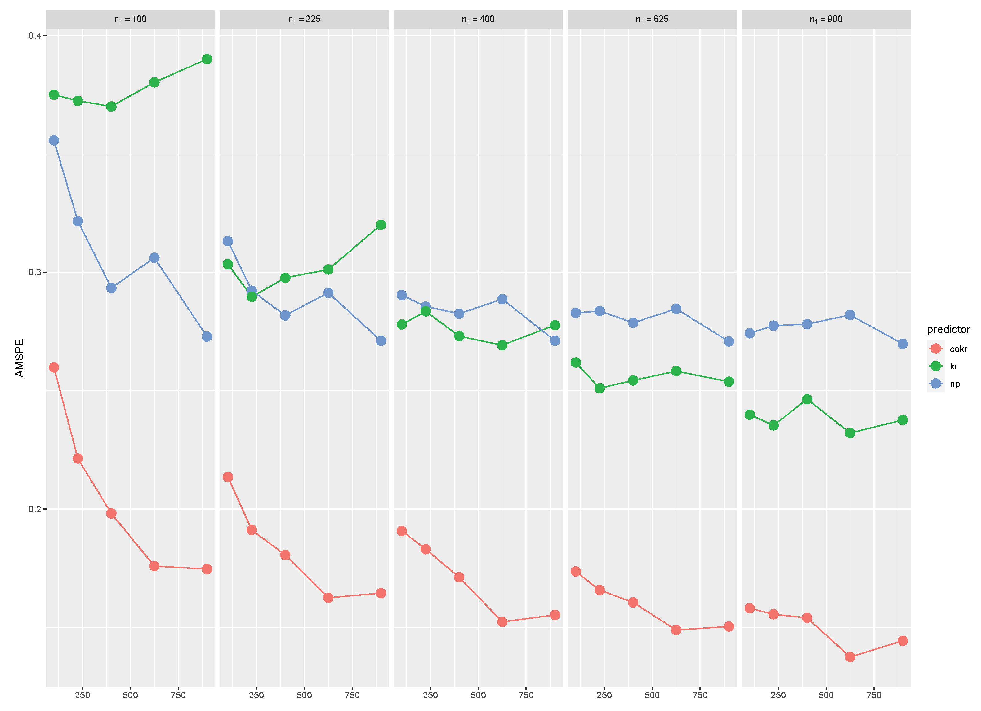
Table 2 and
Figure 1 display the results achieved for the AMSPE, with several sizes
and
, where a similar pattern to the one previously described is shown. Indeed, those methods that make use of the auxiliary data (cokriging and nonparametric predictors) yield the smallest errors and they decrease for larger sizes
and
, with a slight outperformance of the cokriging approach over the nonparametric one. This fact may again be due to the favorable scenario designed for the cokriging technique, although the difference between both procedures tends to diminish as
and
increase.
Thus, the first study confirms some benefits of using the cokriging technique, when Gaussian processes are considered, with a correct specification of the estimated trend and spatial dependence. Then, a further step in our research is addressed to analyze the development of the new methodology for prediction, under deviations from the aforementioned features.
We started by checking the effect of misspecification in the parametric estimation of the semivariogram functions. For the latter purpose, in the second study, bivariate data were drawn from independent Gaussian processes
and
, with isotropic exponential (Exp) and Matérn (Mat) semivariograms, respectively. The Matérn model involves an additional parameter
and the particular choice of
provides the exponential model. To generate the samples in our analyses, we considered constant trends
and
, as well as the semivariogram parameters
and
, for
, together with
for the Matérn function. The cross-semivariograms
were obtained as given in (
12), through several combinations of semivariogram models selected for
and
, which include the theoretical ones (Exp-Mat), as well as misspecified alternatives obtained by considering the spherical (Sph) family for
or the Gaussian (Gau) family for
.
Figure 2 depicts the form of the cross-semivariograms employed in the current study, so that the functions derived under a correct specification of the theoretical model are compared with their counterparts, achieved with a partially misspecified model (
Figure 2a) and a totally misspecified one (
Figure 2b). These plots show that the wrong selection of the parametric families leads to inaccurate estimates of the semivariograms at small distances, with the largest deviations observed for the totally misspecified scenario, as expected, for which the resulting nuggets clearly differ from the corresponding values attained through the theoretical model. These variations of the semivariograms estimates at lags close to zero should have a noticeable effect on prediction, which was checked in the analysis described below.
Table 3 presents the results of the second numerical study, addressed to compare the performance of the three prediction approaches, under different specifications of the dependence structure. As expected, the use of the theoretical models (Exp-Mat) gives rise to the best results, with the smallest errors attained through the cokriging and the nonparametric methods, showing some distance to the corresponding values provided by the kriging predictor. On the other hand, the misspecification does not have an effect on the new methodology for prediction, unlike what happens to the other procedures. Indeed, the wrong selection of one of the semivariogram models (Exp-Gau) leads to an augment in the errors derived through the kriging and cokriging techniques. This trend is even more evident when using a totally misspecified model (Sph-Gau), which results in an additional increment of the AMSPE values obtained.
In the previous studies, the trends
and
were taken as constant values, so the third analysis is focused on exploring the performance of the three methods considered for prediction under non-constant trend. With this aim, data were generated from model (
11), with the same characteristics as in the second study, except that now linear trends were selected, given by
, for
and
.
Table 4 shows the errors achieved with the proposed nonparametric predictor and the cokriging approach. In the former case, the trend was nonparametrically estimated, whereas for the cokriging predictor, the approximation of the trend was developed through a constant and a linear models.
The results in
Table 4 reflect that the misspecification of the trend models yields the largest errors, even though the cokriging approach was implemented with the right models for the semivariograms. On the other hand, under a correct characterization of the trend, the cokriging and the nonparametric predictors have a similar performance, with a slight superiority of the former one. In this respect, recall the advantages given to the cokriging prediction in this scenario, since this technique is optimal under gaussianity from the random processes, together with the fact that the dependence structures and trends involved in this approach were correctly specified.
In the final numerical study, our aim was to analyze the effects that the deviations from gaussianity might have on the results achieved with the three predictors considered in the current research. Thus, to simulate a non-Gaussian bivariate process, modeled as in (
11), we drew non-Gaussian processes
and
, by taking them as
, for some Gaussian processes
, with zero mean and unit variance, for
. This way of proceeding led to non-Gaussian but stationary random fields
, with mean 1, variance 2 and semivariogram
, where
stands for the semivariogram of
. In particular, for data generation in the current analysis,
and
were selected to have the same characteristics as
in the second study, so their semivariograms followed the isotropic exponential and Matérn models, respectively, with parameters
,
and
, for
. The results are summarized in
Table 5.
The errors displayed in
Table 5 give account of the best performance of the nonparametric predictor over the kriging and cokriging techniques, when the underlying distribution of the random processes
and
departs from gaussianity. Indeed, several problems arise in this scenario with the application of the kriging and cokriging methods. On the one hand, these approaches are no longer optimal for non-Gaussian processes and, on the other, their behavior is highly dependent on the use of proper specifications of the trend and the semivariogram functions.
5. Assessment of Cd Concentrations in the Floodplain of the Meuse River
Now, we describe the application of the proposed methodology to assess the contamination by Cd in the geographical area associated to the Meuse data set. These data, presented in [
34], contain measurements of different pollutants (zinc, cadmium, lead, copper or organic matter, among others), taken on alluvial soils in the floodplain of the Meuse river, close to Stein (Netherlands). A map of the zone is displayed in
Figure 3, designed with the
RgoogleMaps package [
35] of the
R library, which shows the 155 sampling locations considered for data collection.
The aforementioned sample has been studied with different aims and methods, which include the application of the cokriging techniques. An example can be found in [
36], where cokriging was employed with lead (Pb) as target variable and organic matter or zinc as separate auxiliary variables. In the current research, we focused our attention on Cd, since it represents a risk to human health, with the aim of mapping the concentrations of this pollutant on the whole area of interest. This task was accomplished by using the collected Cd and Pb values, due to the association between both elements, whose correlation coefficient with the available data amounted to 0.7989.
A preliminary analysis of the Cd and Pb data depicted asymmetry, thus they were log-transformed to continue the study, where we applied the universal cokriging and the proposed nonparametric tool. The former approach was implemented by fitting a linear model of coregionalization with isotropic exponential semivariograms.
For the choice of bandwidth
h in (
6), as given in (
10), we randomly divided the set of sampling sites into two disjoint subsets, one for training (with 132 sites) and the other for validation (with 23 sites), marked on
Figure 3 as points and crosses, respectively. To proceed in this way, we first selected the spatial locations for the training set from the whole set of sampling sites and the remaining locations formed the validation set. In addition, aiming to solely use the value of one variable at each site, the training set was again split into two separate groups, so that we just considered the values of Cd collected at one of them (with 52 sites) and those of Pb at the other (with 80 sites), represented by red and green points on
Figure 3, respectively. The resulting training data set was used to compute predictor (
6) with different bandwidths and then we selected the one that best approximated the log-values of the Cd concentrations at the validation set. The bandwidth
achieved was employed to proceed with the new methodology.
Finally, the predictions derived with the data in the log-scale and both procedures were back-transformed to the original scale. The results attained for the Cd concentrations (in mg/kg soil), on the geographical area associated to the Meuse data set, are represented in
Figure 4. To measure the accuracy of each mechanism, the AMSPE values were computed at the validation set and they amounted to 2.2737 and 0.8189 for the cokriging and the nonparametric approaches, respectively, thus giving advantage to the latter one.
The maps displayed in
Figure 4 give evidence of the differences between the two prediction methods considered in the current study, although they also exhibit some common patterns. On the one hand, the area with the smallest levels of Cd, identified with the dark blue color, is located in each case on the central part of the region, towards the eastern border, being of larger size the one achieved with the universal cokriging. Then, as we move away from each of the aforementioned areas, the predicted Cd content increases and the highest values are mainly concentrated on the western border of each domain and its vicinity. Nevertheless, the resulting hot spots range in different magnitudes for the two prediction approaches, so that the universal cokriging provides the largest Cd accumulations, even surpassing the green color scale and reaching values above 3 mg/kg soil, unlike what happens to the non-parametric method.
In summary, both ways of proceeding allow the identification of those zones that pose a threat to the population health for their pollutant content. However, the smaller error (AMSPE) achieved by the nonparameric procedure and its good theoretical properties present this predictor as a better candidate for assessment of the points at risk and the consequent decision-making.
6. Conclusions
The current work deals with the construction of a prediction map that shows the concentrations of a pollutant, the cadmium, in the whole region of interest. This issue may be addressed by using the available data of the target variable (Cd) and also incorporating information of a secondary correlated one (Pb), collected at various spatial sites. In geostatistics, problems of this kind are typically solved through the kriging or the cokriging techniques, depending on whether data of one or more variables are employed, respectively. These methods are optimal for Gaussian processes, although their practical implementation requires an appropriate characterization of the underlying dependence structure. This is not an easy task to be accomplished, specially when cokriging is applied, due to the number of functions to be approximated and the properties that the resulting estimates must satisfy. Thus, our research introduces an alternative kernel-type approach for spatial prediction with covariables, which was designed to overcome the previous drawbacks. Indeed, the new methodology just involves p cross-covariances (or cross-semivariograms), for a p-variate random process, instead of the functions of more complex estimation that are needed for cokriging. To characterize the aforementioned p functions, as well as other unknown terms in our proposal, such as those dependent on the trends, we recommend proceeding through nonparametric procedures, to avoid the misspecification problem present in the parametric estimation. The choice of bandwidths, required to implement the kernel predictor, is also addressed in the current work. In particular, we propose a cross-validation method to derive a global bandwidth h, based on considering random training and validation sets. However, further research should be developed to analyze alternative mechanisms for the selection of sites to be included in each set and, even, to provide additional approaches for bandwidth selection, which could be derived from the application of the bootstrap methodology. The numerical studies carried out in the current study give account of the sensitivity of the kriging and the cokriging techniques to the proper specification of the trend and the cross-semivariograms, unlike what happens to the nonparametric predictor. In addition, deviations from gaussianity in the data are less noticeable when prediction is developed with the new methodology than with the other approaches. Then, the use of the nonparametric proposal is recommended over the cokriging to obtain more accurate predictions of the Cd concentrations, with Pb as auxiliary variable, so as to detect those areas with highest accumulation of Cd, which is crucial for health protection.


