A Risk-Aversion Approach for the Multiobjective Stochastic Programming Problem

Abstract

Multiobjective stochastic programming is a field that is well suited to tackling problems that arise in many fields: energy, financial, emergencies, among others; given that uncertainty and multiple objectives are usually present in such problems. A new concept of solution is proposed in this work, which is especially designed for risk-averse solutions. The proposed concept combines the notions of conditional value-at-risk and ordered weighted averaging operator to find solutions protected against risks due to uncertainty and under-achievement of criteria. A small example is presented in order to illustrate the concept in small discrete feasible spaces. A linear programming model is also introduced to obtain the solution in continuous spaces. Finally, computational experiments are performed by applying the obtained linear programming model to the multiobjective stochastic knapsack problem, gaining insight into the behaviour of the new solution concept.

1. Introduction

Decision making is never easy, yet we often have to make decisions. Emergencies and disaster management are fields in which many difficulties often arise, such as high uncertainty and multiple conflicting objectives. Risk-averse decisions are usually sought to overcome such difficulties. Risk-aversion is the attitude for which we prefer to lower uncertainty rather than gambling extreme outcomes (positive or negative).

Risk-aversion, although typically studied in problems with uncertainty, can as well be considered when making decisions with multiple criteria. For instance, in the field of disaster management, solutions that are sufficiently good for all criteria are usually preferred to others that perform exceptionally good for some criteria, but inadequately for the others.

Multicriteria decision making (MCDM) is a field worth of consideration when studying real-world problems. This situation, in which multiple conflicting objectives have to be optimized, has led to the definition of different solution concepts and methodologies. A specific methodology should be applied depending on the problem and the type of solution considered. A key concept in MCDM is the notion of efficiency, which reflects the intuition that, for a solution to be acceptable, another cannot exist improving that one in every objective.

Uncertainty is another feature that is present in the studied problems, in which risk-averse decisions will be preferred. The most common ways for dealing with the uncertainty are stochastic programming and robust optimization, in which fuzzy optimization is also included [1]. Stochastic programming is the widest used technique when there are historical data or information to infer a probability distribution. Moreover, usually discrete distributions are used, calling scenarios the different values. The concepts of value-at-risk (VaR) and conditional value-at-risk (CVaR) are widely used for quantifying risk. They are typically defined for losses distributions in finance, where the right tail of the distributions are of interest.

Consider now the following problem, in which multiple objectives to be minimized and uncertainty are included simultaneously:

$$\underset{x\in X}{min}\left(f_1(x,\omega ),\dots ,f_K(x,\omega )\right)$$

The above problem is typically called multiobjective stochastic programming problem (MSP), especially if $\omega$, the uncertainty source, has a known probability distribution.

In this paper, we introduce a new solution concept in multiobjective stochastic programming based on risk-averse preferences. Such a concept is complemented with a mathematical programming model in order to compute it efficiently, and computational experiments are performed to assess its strengths.

The remaining of this paper is organized as follows. Section 2 presents a literature review of multicriteria decision-making and uncertain optimization. Section 3 includes the definition of a novel concept of solution for MSP problems and studies its properties. In Section 3.2, such a solution concept is illustrated with a basic example when the decision space is finite and small.

Section 4 shows how to obtain such a solution with a linear programming model. An application to the multicriteria knapsack problem is developed in Section 5, and general conclusions of the research are drawn in Section 6.

2. Literature Review

2.1. Multicriteria Decision-Making and Optimization under Uncertainty

MCDM techniques have recently been used for solving real world problems as varied as: disaster management [2,3], engineering [4], finance [5,6], forest planning [7], healthcare [8], location of waste facilities [9], police districting [10], route planning [11], train scheduling [12], or urban planning [13,14].

An important concept used throughout this paper is the one of efficiency. The notation used is the given in [15]:

Definition 1

(Efficiency, [15]). Let $f_1(x),\dots ,f_K(x)$ be objective functions to be minimized, and let X be the feasible set. A feasible solution $\widehat{x}\in X$ is called:

• Weakly efficient if there is no $x\in X$, $x\ne \widehat{x}$, such that $f(x)<f(\widehat{x})$ i.e., $f_k(x)<f_k(\widehat{x})$ for all $k=1,\dots ,K$.
• Efficient or Pareto optimal if there is no $x\in X$ such that $f_k(x)\le f_k(\widehat{x})$ for all $k=1,\dots ,K$ and $f_i(x)<f_i(\widehat{x})$ for some $i\in \{1,\dots ,K\}$.
• Strictly efficient if there is no $x\in X$, $x\ne \widehat{x}$, such that $f(x)\le f(\widehat{x})$.

The different approaches for dealing with uncertainty do not respond to the desires of the modeller; instead, they reflect the nature of the uncertainty. If the uncertainty comes with an underlying known or estimated probability distribution, then stochastic programming is used. For an introduction to stochastic programming, the reader is referred to [16]. On the other hand, if uncertainty comes from a lack of precision or semantic uncertainty, then robust optimization is used. Robust optimization does not assume a known (or existing) distribution [17,18,19]. A recent review of robust optimization is written in [20].

Stochastic programming seeks the optimization of a characteristic value of a random variable, usually its average. However, in risk-averse contexts the usage of value-at-risk and conditional value-at-risk is common for quantifying risk (see, for instance, [21,22,23,24,25]).

Definition 2

(CVaR, [26]). Given $F_X(x)$ distribution function, and $\beta \in [0,1]$, the β-CVaR is the conditional expected value over $\{x:F_X(x)\ge \beta \}$.

2.2. Multiobjective Stochastic Programming

Multiobjective stochastic programming refers to models in which there are several criteria and stochastic uncertainty simultaneously. Reference [27] develops the PROTRADE method, where utility functions are defined to aggregate objectives into a single objective stochastic problem. The resulting problem is solved with an interactive method, where the decision-maker defines an expected solution and a feasibility probability. Reference [28] reduces the stochasticity by adding some good measures to the list of objectives, such as the mean, variance, or probability of being over/below a threshold. The resulting multiobjective deterministic problem is solved aggregating the objectives, but it could be solved via other techniques.

Reference [29] compares the stochastic approach with the multiobjective approach when using different techniques. The stochastic approach transforms the MSP on a single-objective stochastic problem, while the multiobjective approach first reduces the stochasticity transforming the MSP on a deterministic multiobjective problem. They highlight that “the multiobjective approach forgets the possible existence of stochastic dependencies between objectives”. Reference [30] studies stochastic goal programming, where the deviation of the objective functions to some goals set beforehand to stochastic values is minimized.

In [31], a chance-constrained compromise approach is proposed, with an example presented in  [32]. In [33], the INTEREST method is proposed. It is an interactive reference point method. The decision-maker gives reference levels $u_i$ and probabilities ${\beta }_i$, hoping to achieve a solution $x^{*}$ such that $\mathbb{P}\left(f_i(x^{*})\le u_i\right)\ge {\beta }_i$. If this is infeasible, then the decision-maker should either increase the reference levels or decrease the probabilities of achievement. [34] reviews different solutions methods for the MSP problem, categorizing them as stochastic approach or multiobjective approach. Reference [35] surveys methods for MSP problems that do not reduce the multiple objectives before the analysis of the problem, acknowledging the difficulty of risk-averse decision-making. More recently, in [36], different ordering relations for multicriteria problems with uncertainty are presented, building upon existing notions of robustness.

Some fields where MSP models have been developed are: forest management [37], multiple response optimization [38], energy generation [39,40], energy exchange [41], capacity investment [42], disaster management [43,44], portfolio optimization [45], and cash management [46], among others.

3. Methodology

The concept of CVaR allows aggregating several scenarios by just looking at what happens in the worst ones. The ordered weighted averaging (OWA) operators are defined in [47], and independently in the field of locational analysis [48,49] under the name of ordered median function. These concepts will allow for us to aggregate different criteria by looking at the least desirable ones, as a risk-aversion measure.

Definition 3

(OWA, [47]). Given $a_1,\dots ,a_n\in \mathbb{R}$, the ordered weighted averaging (OWA) operator with weights ${\lambda }_1,\dots ,{\lambda }_n$ is defined as:

$$OWA(a_1,\dots ,a_n)=\sum _i{\lambda }_i{a}_{(i)}$$

where $\left(a_{(1)},\dots ,a_{(n)}\right)$ is the ordered vector from largest to smallest $\left(a_1,\dots ,a_n\right)$.

Remark 1.

For certain weights, the OWA represents a known quantity:

• If ${\lambda }_i=\frac{1}{n}$, the resulting OWA is the average of a.
• If ${\lambda }_1=1$, and ${\lambda }_j=0$ for $j>1$, the OWA is the maximum of a.
• If ${\lambda }_n=1$, and ${\lambda }_j=0$ for $j<n$, the OWA is the minimum of a.

Reference [50] later studies how to assign weights for an OWA when criteria have different importances.

Definition 4

(OWA with importances, [50]). Given $a_1,\dots ,a_n\in \mathbb{R}$ with importances $u_1,\dots ,u_n$ such that ${\sum }_i{u}_i=1$ the weights ${\lambda }_j$ for the OWA can be calculated with f, the weight generating function in the following manner:

1. 

Sort vector a such that $a_{(1)}\ge a_{(2)}\ge \dots \ge a_{(n)}$.

2. 

With $(\times )$ as the order induced by a, define $T_j={\sum }_{k=1}^j{u}_{(k)}$.

3. 

Let f be a function, such that $f:[0,1]\to [0,1]$ and $f(0)=0,f(1)=1$. This function is called weight generating function.

4. 

Obtain the weights as ${\lambda }_j=f(T_j)-f(T_{j-1})$.

Example 1 (of Definition 4).

Consider the following weight generating function, for a given $r\in (0,1]$:

$$f(x)=\left\{\begin{array}{cc}\frac{x}{r}\hfill & ifx<r\hfill \\ 1\hfill & ifx\ge r\hfill \end{array}\right.$$

(1)

Let $(\times )$ be the order, such that $a_{(1)}\ge \dots \ge a_{(n)}$, $u_{(j)}$ the weight associated to $a_{(j)}$, and also let $T_j={\sum }_{k=1}^j{u}_{(k)}$. We shall now see how the weights are obtained from f. Let $j^{*}$ be such that $T_{j^{*}-1}<r\le T_{j^{*}}$.

• ${\lambda }_1=f(T_1)=f(u_{(1)})=\frac{u_{(1)}}{r}$, assuming $u_{(1)}<r$
• ${\lambda }_2=f(T_2)-f(T_1)=f(u_{(1)}+u_{(2)})-f(u_{(1)})=\frac{u_{(1)}+u_{(2)}}{r}-\frac{u_{(1)}}{r}=\frac{u_{(2)}}{r}$, assuming $u_{(1)}+u_{(2)}<r$
• …
• ${\lambda }_{j^{*}}=f(T_{j^{*}})-f(T_{j^{*}-1})=1-\left(\frac{u_{(1)}+u_{(2)}+\dots +u_{(j^{*}-1)}}{r}\right)$, since $T_{j^{*}}\ge r$
• ${\lambda }_{j^{*}+1}=f(T_{j^{*}+1})-f(T_{j^{*}})=1-1=0$
• …
• ${\lambda }_n=f(T_n)-f(T_{n-1})=1-1=0$

Consequently the OWA of $a_1,\dots ,a_n$ with importances $u_1,\dots ,u_n$ is:

$$\begin{array}{cc}\hfill OWA=& \frac{u_{(1)}}{r}{a}_{(1)}+\frac{u_{(2)}}{r}{a}_{(2)}+\dots +\left[1-\left(\frac{u_{(1)}+u_{(2)}+\dots +u_{(j^{*}-1)}}{r}\right)\right]a_{(j^{*})}\hfill \\ \hfill =& \frac{u_{(1)}{a}_{(1)}+u_{(2)}{a}_{(2)}+\dots +\left(r-u_{(1)}-u_{(2)}-\dots \right)a_{(j^{*})}}{r}\hfill \end{array}$$

That is, the OWA that is characterized by the weight generating function given in (1) is the average of the worst $a_j$, weighted by their importances, with the total importance adding up to r. The values of λ reflect the preferences of the decision-maker. The parameter r leads to incorporating the different attributes, from worst to best, until a threshold is reached.

The starting point of this paper is the recurrent idea of representing ordered weighted or ordered median operators while using k-sums. k-sums (or k-centra in the location analysis literature) are sums of the k-largest terms of a vector [51]. One can trace back, at least to [52], the use of k-sums to represent ordered median objectives. More recent references are, for instance, [53,54,55,56]. This last reference introduces a normalized version of k-centrum, named $\beta$-average, which will be used in our paper.

Through the remaining of the paper, consider that $f_k^j(x)$ are functions to be minimized within a feasible set X, with $k=1,\dots ,K$ representing K different objectives with importances $w_k$ and $j=1,\dots ,$J encoding J different scenarios with probabilities ${\pi }_j$.

Definition 5

($\beta$-average, $g_k^{\beta }(x)$, [56]). Given $\beta \in (0,1]$, for each criterion k it can be defined $g_k^{\beta }(x)$ which measures the average of f on the worst scenarios $\left(f_k^1(x),\dots ,f_k^J(x)\right)$, with accumulated probability equal to β.

Remark 2

([56]). Given a value β, if the sum of the probabilities of the worst scenarios is exactly β, then the β-average is exactly $\left(1-\beta \right)$-CVaR.

Example 2.

Consider a point x, a fixed criterion k, and five different scenarios with probabilities ${\pi }_j$ and values of $f_k^j$ given.

Table 1. Small example of $\beta$-average for different values of $\beta$.

	Scenario					$\mathit{\beta }$
	1	2	3	4	5	0.2	0.3	0.5
${\pi }_j$	0.2	0.1	0.3	0.25	0.15	10	9	7
$f_k^j(x)$	10	7	4	3	2

shows the β-averages for different values of β, in which the scenarios have been ordered from largest value of f to smallest.

• For $\beta =0.2$, the scenario $j=1$ is the only one needed to obtain the worst scenario with probability $0.2$, and hence $g_k^{\beta }(x)=\frac{0.2\times 10}{0.2}=10$.
• When β equals 0.3 it is necessary to include scenario 2, obtaining a β-average of $\frac{0.2\times 10+0.1\times 7}{0.3}=9$.
• Finally, if $\beta =0.5$ scenario 3 needs to be added as well, but only with the probability needed until reaching $0.5$: $g_k^{\beta }(x)=\frac{0.2\times 10+0.1\times 7+0.2\times 4}{0.5}=7$.

When using the $\beta$-average the functions $f_k^j(x)$ were transformed into $g_k^{\beta }(x)$, a collection of K functions not depending on the scenario. An OWA will be defined now, via its weight generating function, which will reduce the K $\beta$-averages into a scalar function.

Definition 6 (r-OWA, $O_r(\overrightarrow{x})$)

Given $x_1,\dots ,x_K\in \mathbb{R}$ with importances $w_1,\dots ,w_K$, such that ${\sum }_{k=1}^K{w}_k=1$ and $r\in (0,1]$, the function $O_r(\overrightarrow{x})$ is defined as the OWA with the following weight generating function:

$$f(x)=\left\{\begin{array}{cc}\frac{x}{r}\hfill & ifx<r\hfill \\ 1\hfill & ifx\ge r\hfill \end{array}\right.$$

Remark 3.

The definition of $O_r(\overrightarrow{x})$ is made in a similar manner that the one given of the β-average (Definition 5), but it is done on a context with importances rather than probabilities. Example 3 shows the similarities between both of the approaches.

Example 3.

Consider a point x and let $g_k(x)$ be the evaluation of x under five different criteria with importances $w_j$.

Table 2. Small example of r-OWA for different values of r.

	Criterion					r
	1	2	3	4	5	0.2	0.3	0.5
$w_k$	0.2	0.1	0.3	0.25	0.15	10	9	7
$g_k(x)$	10	7	4	3	2

shows the r-OWAs for different values of r, in which the criteria have been ordered from largest values of $g_k(x)$ to smallest. Consider the case $r=0.5$:

1. 

As $g_k(x)$ are already ordered for largest to smallest, the values of $T_k$ are:

$$T_1=0.2,T_2=0.2+0.1=0.3,T_3=0.6,T_4=0.85,T_5=1$$

2. 

The values of $T_k$ under f:

$$f(T_1)=\frac{0.2}{0.5},f(T_2)=\frac{0.3}{0.5},f(T_3)=f(T_4)=f(T_5)=1$$

3. 

The weights of the OWA:

$${\lambda }_1=\frac{0.2}{0.5},{\lambda }_2=\frac{0.3-0.2}{0.5}=\frac{0.1}{0.5},{\lambda }_3=1-\frac{0.3}{0.5}=\frac{0.2}{0.5},{\lambda }_4={\lambda }_5=0$$

4. 

Consequently, the r-OWA is:

$$r\text{-}OWA=\frac{0.2g_{(1)}(x)+0.1g_{(2)}(x)+0.2g_{(3)}(x)}{0.5}=\frac{0.2\times 10+0.1\times 7+0.2\times 4}{0.5}=7$$

Remark 4.

Given $x_1,\dots ,x_K$ and its associated importances $w_1,\dots ,w_K$, then the ${\lambda }_k$ of the r-OWA are ${\lambda }_k=\frac{{\tilde{\lambda }}_k}{r}$, with ${\tilde{\lambda }}_k$ being determined as:

$$O_r(x_1,\dots ,x_K)=\underset{{\tilde{\lambda }}_1,\dots ,{\tilde{\lambda }}_K}{max}\left\{\frac{{\tilde{\lambda }}_1{x}_1+\dots +{\tilde{\lambda }}_K{x}_K}{r}\mid {\tilde{\lambda }}_k\le w_k,\sum {\tilde{\lambda }}_k=r\right\}$$

Given $r,\beta \in (0,1]$ and $x\in X$, let us introduce the function $h_r^{\beta }(x)$ as the r-OWA of the $\beta$-averages. That is:

$$h_r^{\beta }(x)=O_r\left(g_1^{\beta }(x),\dots ,g_K^{\beta }(x)\right)$$

Remark 5.

If the importance of all the criteria is the same ($w_k=\frac{1}{K}$ for all k) and $r=\frac{n}{K}$ with $n\in \{1,\dots ,K\}$, then $h_r^{\beta }(x)$ is the average of the n worst β-averages. Recall that this is called n-centra [57].

Definition 7 (Dominance).

Let x and y feasible solutions ($x,y\in X$) and $r,\beta \in (0,1]$. Then x dominates y ($x\succsim y$) if $h_r^{\beta }(x)\le h_r^{\beta }(y)$, where $h_r^{\beta }(x)$ is the r-OWA of the β-averages.

Definition 7 induces a domination relationship with the following properties:

Reflexivity 

   Given x, $h_r^{\beta }(x)\le h_r^{\beta }(x)$, and then $x\succsim x$, so ≿ is reflexive.

Transitiveness 

Given $x\succsim y$, $y\succsim z$, we have $h_r^{\beta }(x)\le h_r^{\beta }(y)$ and $h_r^{\beta }(y)\le h_r^{\beta }(z)$, and then $h_r^{\beta }(x)\le h_r^{\beta }(z)$, which leads to $x\succsim z$, and we conclude that ≿ is transitive.

Antisymmetry 

Given $x\succsim y$, $y\succsim x$, we have $h_r^{\beta }(x)\le h_r^{\beta }(y)$ and $h_r^{\beta }(y)\le h_r^{\beta }(x)$, but, from $h_r^{\beta }(x)=h_r^{\beta }(y)$, it cannot be guaranteed that $x=y$, and, hence, ≿ is not antisymmetric.

3.1. Idea of Solution and Dominance Properties

Consider the multiobjective stochastic programming problem:

$$\underset{x\in X}{min}\left(f_1(x,\omega ),\dots ,f_K(x,\omega )\right)$$

The previously defined concepts of $\beta$-average and r-OWA transform the $MSP$ problem into a deterministic multiple objective problem, and then into a deterministic single objective problem.

$$MSP\to MOP\to LP(MIP)$$

$$f_k^j(x)\stackrel{\beta \text{-}\mathrm{average}}{\to }{g}_k^{\beta }(x)\stackrel{r\text{-}\mathrm{OWA}}{\to }{h}_r^{\beta }(x)$$

• For every $x\in X$ there is a function $f_k^j$ to be minimized which depends on the scenario j and the criterion k.
• The problem is transformed into a deterministic one with multiple objectives (MOP) while using the $\beta$-average concept.
• When computing the r-OWA, each $x\in X$ is assigned a scalar. The problem consists of finding the x, which minimizes this $h_r^{\beta }(x)$.

The solution procedure lies into what is usually called a scalarization approach. When obtaining a minimizer of $h_r^{\beta }(x)$, it is also desired that the optimal solution is efficient for the associated MOP problem:

$$\underset{x\in X}{min}\left(g_1^{\beta }(x),\dots ,g_K^{\beta }(x)\right)$$

(MOP)

Proposition 1.

Given $x^{*}$ minimum of $h_r^{\beta }(x)$ the following statements hold:

1. 

$x^{*}$ is not necessarily efficient of the MOP problem.

2. 

$x^{*}$ is weakly efficient of the MOP problem.

3. 

If $x^{*}$ is the only minimum of $h_r^{\beta }(x)$, then $x^{*}$ is efficient.

4. 

Given $x^{*}$ not efficient, an alternative $y^{*}$ can be found on a second phase, such that $y^{*}$ is efficient and $h_r^{\beta }(x^{*})=h_r^{\beta }(y^{*})$.

These properties are known when using scalarization techniques [15]. Hence, only an example of the first statement will be shown.

Example 4 ($x^{*}$ is not necessarily efficient).

Consider the example that is displayed in

Table 3. Values of two alternatives for each scenario j and criterion k, together with their $\beta$-averages ($\beta =\frac{1}{2}$) and r-OWAs ($r=\frac{2}{3}$).

(a) Alternative 1				(b) Alternative 2
	$k_1$	$k_2$	$k_3$		$k_1$	$k_2$	$k_3$
$j_1$	0.80	0.40	0.30	$j_1$	0.70	0.45	0.65
$j_2$	0.60	0.20	0.65	$j_2$	0.80	0.30	0.50
$\beta$-average	0.80	0.40	0.65	$\beta$-average	0.80	0.45	0.65
r-OWA	0.725			r-OWA	0.725

, in which there are only two feasible solutions, two equiprobable scenarios (${\pi }_1={\pi }_2=\frac{1}{2}$), three equally important criteria ($w_1=w_2=w_3=\frac{1}{3}$), and consider the values of $\beta =\frac{1}{2}$ and $r=\frac{2}{3}$ are taken.

The β-averages are $(0.8,0.4,0.65)$ for the first alternative and $(0.8,0.45,0.65)$ for the second alternative. When computing the function $h_r^{\beta }$, both of the alternatives have an objective value of $0.725$. Consequently, even though the second alternative is an optimal solution of $h_r^{\beta }$, it is not an efficient solution of the MOP problem as its β-averages are dominated by those of the first alternative.

The transformation of the problem from a multiple objective one to a single objective one is done using weights. These weights correspond to a subjective scale that is introduced by the expert, representing the importance of the criteria considered in the problem as accurately as possible.

3.2. An Illustrative Example

The proposed solution concept will now be applied, first with a discrete (and small) case. When the solution space is discrete, and all feasible solutions can be explicitly enumerated, the steps are as  follows:

Step 0 

Normalize all objective functions $f_k^j(x)$.

Step 1 

Set values for $\beta ,r\in (0,1]$.

Step 2 

For every $x\in X$ and every criterion define $g_k^{\beta }(x)$ as:

$$g_k^{\beta }(x)=\begin{array}{l}\mathrm{average}\mathrm{of}\mathrm{worst}\mathrm{scenarios}\mathrm{for}\mathrm{criterion}k\\ \mathrm{with}\mathrm{probabilities}\mathrm{adding}\mathrm{up}\mathrm{to}\beta \end{array}$$

Step 3 

Define $h_r^{\beta }(x)$ as:

$$h_r^{\beta }(x)=\begin{array}{l}average of worst g_k^{\beta }(x) values\\ with importances adding up to r\end{array}$$

Step 4 

Search for $x\in X$ minimizing $h_r^{\beta }(x)$.

Assume a decision space with only four alternatives, evaluated under five different scenarios with six criteria. For each of those alternatives, it can be computed the value of the functions $f_k^j(x)$ to be minimized.

Table 4. Values of alternative 1 by scenario (j) and criteria (k).

			Criteria
			${\mathit{w}}_{\mathbf{1}}=\mathbf{0.20}$	${\mathit{w}}_{\mathbf{2}}=\mathbf{0.10}$	${\mathit{w}}_{\mathbf{3}}=\mathbf{0.20}$	${\mathit{w}}_{\mathbf{4}}=\mathbf{0.25}$	${\mathit{w}}_{\mathbf{5}}=\mathbf{0.15}$	${\mathit{w}}_{\mathbf{6}}=\mathbf{0.10}$
			${\mathit{k}}_{\mathbf{1}}$	${\mathit{k}}_{\mathbf{2}}$	${\mathit{k}}_{\mathbf{3}}$	${\mathit{k}}_{\mathbf{4}}$	${\mathit{k}}_{\mathbf{5}}$	${\mathit{k}}_{\mathbf{6}}$
scenarios	${\pi }_1=0.15$	$j_1$	0.51	0.27	0.39	0.45	0.75	0.76
	${\pi }_2=0.20$	$j_2$	0.58	0.65	0.47	0.26	0.90	0.24
	${\pi }_3=0.30$	$j_3$	0.48	0.44	0.90	0.50	0.93	0.65
	${\pi }_4=0.25$	$j_4$	0.76	0.18	0.01	0.90	0.56	0.02
	${\pi }_5=0.10$	$j_5$	0.86	0.36	0.21	0.28	0.63	0.72

shows the values of f, evaluated on the feasible point $x_1$, by each of the scenarios and criteria considered.

The first step is calculating the $\beta$-averages. Let us assume a value of $\beta =0.3$:

• For the first criterion the worst scenario is $j_5$, which has probability $0.1$. The second worst is $j_4$, with a probability of $0.25$. As the sum of those probabilities exceeds the $\beta$ fixed, for computing the $\beta$-average just a probability of $0.2$ is considered:

  $$g_1^{\beta }(x_1)=\frac{0.1\times 0.86+0.2\times 0.76}{0.3}=0.793$$
• $g_2^{\beta }(x_1)=\left(0.2\times 0.65+0.1\times 0.44\right)/0.3=0.580$
• $g_3^{\beta }(x_1)=\left(0.3\times 0.90\right)/0.3=0.900$
• $g_4^{\beta }(x_1)=0.833$, $g_5^{\beta }(x_1)=0.930$, $g_6^{\beta }(x_1)=0.728$

The last step is calculating the function $h_r^{\beta }(x)$, which is, the r-OWA of the $\beta$-averages.

Table 5. Values of alternative 1 by scenario (j) and criteria (k).

			Criteria
			${\mathit{w}}_{\mathbf{1}}=\mathbf{0.20}$	${\mathit{w}}_{\mathbf{2}}=\mathbf{0.10}$	${\mathit{w}}_{\mathbf{3}}=\mathbf{0.20}$	${\mathit{w}}_{\mathbf{4}}=\mathbf{0.25}$	${\mathit{w}}_{\mathbf{5}}=\mathbf{0.15}$	${\mathit{w}}_{\mathbf{6}}=\mathbf{0.10}$
			${\mathit{k}}_{\mathbf{1}}$	${\mathit{k}}_{\mathbf{2}}$	${\mathit{k}}_{\mathbf{3}}$	${\mathit{k}}_{\mathbf{4}}$	${\mathit{k}}_{\mathbf{5}}$	${\mathit{k}}_{\mathbf{6}}$
scenarios	${\pi }_1=0.15$	$j_1$	0.51	0.27	0.39	0.45	0.75	0.76
	${\pi }_2=0.20$	$j_2$	0.58	0.65	0.47	0.26	0.90	0.24
	${\pi }_3=0.30$	$j_3$	0.48	0.44	0.90	0.50	0.93	0.65
	${\pi }_4=0.25$	$j_4$	0.76	0.18	0.01	0.90	0.56	0.02
	${\pi }_5=0.10$	$j_5$	0.86	0.36	0.21	0.28	0.63	0.72
$\beta$-average, $\beta =0.30$			0.793	0.580	0.900	0.833	0.930	0.728
r-OWA, $r=0.17$			0.927

calculates the r-OWA, and also shows the information of the previously calculated $\beta$-averages, when the value of $r=0.17$ is taken.

The values of the functions for the other alternatives, as well as its $\beta$-averages and r-OWAs are shown in

Table A1. Values of alternative 2 by scenario (j) and criteria (k).

			Criteria
			${\mathit{w}}_{\mathbf{1}}=\mathbf{0.20}$	${\mathit{w}}_{\mathbf{2}}=\mathbf{0.10}$	${\mathit{w}}_{\mathbf{3}}=\mathbf{0.20}$	${\mathit{w}}_{\mathbf{4}}=\mathbf{0.25}$	${\mathit{w}}_{\mathbf{5}}=\mathbf{0.15}$	${\mathit{w}}_{\mathbf{6}}=\mathbf{0.10}$
			${\mathit{k}}_{\mathbf{1}}$	${\mathit{k}}_{\mathbf{2}}$	${\mathit{k}}_{\mathbf{3}}$	${\mathit{k}}_{\mathbf{4}}$	${\mathit{k}}_{\mathbf{5}}$	${\mathit{k}}_{\mathbf{6}}$
scenarios	${\pi }_1=0.15$	$j_1$	0.40	0.58	0.39	0.45	0.54	0.18
	${\pi }_2=0.20$	$j_2$	0.68	0.74	0.70	0.15	0.54	0.72
	${\pi }_3=0.30$	$j_3$	0.93	0.52	0.23	0.82	0.21	0.03
	${\pi }_4=0.25$	$j_4$	0.37	0.85	0.07	0.42	0.52	0.22
	${\pi }_5=0.10$	$j_5$	0.92	0.13	0.71	0.39	0.90	0.87
$\beta$-average, $\beta =0.30$			0.930	0.832	0.703	0.820	0.660	0.770
r-OWA, $r=0.17$			0.930

,

Table A2. Values of alternative 3 by scenario (j) and criteria (k).

			Criteria
			${\mathit{w}}_{\mathbf{1}}=\mathbf{0.20}$	${\mathit{w}}_{\mathbf{2}}=\mathbf{0.10}$	${\mathit{w}}_{\mathbf{3}}=\mathbf{0.20}$	${\mathit{w}}_{\mathbf{4}}=\mathbf{0.25}$	${\mathit{w}}_{\mathbf{5}}=\mathbf{0.15}$	${\mathit{w}}_{\mathbf{6}}=\mathbf{0.10}$
			${\mathit{k}}_{\mathbf{1}}$	${\mathit{k}}_{\mathbf{2}}$	${\mathit{k}}_{\mathbf{3}}$	${\mathit{k}}_{\mathbf{4}}$	${\mathit{k}}_{\mathbf{5}}$	${\mathit{k}}_{\mathbf{6}}$
scenarios	${\pi }_1=0.15$	$j_1$	0.80	0.90	0.61	0.28	0.94	0.09
	${\pi }_2=0.20$	$j_2$	0.29	0.48	0.26	0.23	0.21	0.07
	${\pi }_3=0.30$	$j_3$	0.73	0.65	0.32	0.56	0.95	0.65
	${\pi }_4=0.25$	$j_4$	0.58	0.39	0.21	0.66	0.70	0.93
	${\pi }_5=0.10$	$j_5$	0.73	0.22	0.33	0.31	0.32	0.38
$\beta$-average, $\beta =0.30$			0.765	0.775	0.468	0.643	0.950	0.883
r-OWA, $r=0.17$			0.943

and

Table A3. Values of alternative 4 by scenario (j) and criteria (k).

			Criteria
			${\mathit{w}}_{\mathbf{1}}=\mathbf{0.20}$	${\mathit{w}}_{\mathbf{2}}=\mathbf{0.10}$	${\mathit{w}}_{\mathbf{3}}=\mathbf{0.20}$	${\mathit{w}}_{\mathbf{4}}=\mathbf{0.25}$	${\mathit{w}}_{\mathbf{5}}=\mathbf{0.15}$	${\mathit{w}}_{\mathbf{6}}=\mathbf{0.10}$
			${\mathit{k}}_{\mathbf{1}}$	${\mathit{k}}_{\mathbf{2}}$	${\mathit{k}}_{\mathbf{3}}$	${\mathit{k}}_{\mathbf{4}}$	${\mathit{k}}_{\mathbf{5}}$	${\mathit{k}}_{\mathbf{6}}$
scenarios	${\pi }_1=0.15$	$j_1$	0.30	0.52	0.12	0.68	0.46	0.73
	${\pi }_2=0.20$	$j_2$	1.00	0.57	0.46	0.82	0.90	0.72
	${\pi }_3=0.30$	$j_3$	0.18	0.76	0.30	0.34	0.54	0.99
	${\pi }_4=0.25$	$j_4$	0.53	0.21	0.13	0.12	0.66	0.86
	${\pi }_5=0.10$	$j_5$	0.98	0.46	0.50	0.29	0.27	0.40
$\beta$-average, $\beta =0.30$			0.993	0.760	0.473	0.773	0.820	0.990
r-OWA, $r=0.17$			0.993

, starting on Page 21.

Table 6. $\beta$-averages and r-OWAs for each of the four feasible alternatives of the example.

	$\mathit{\beta }$-Averages						r-OWA
	${\mathit{g}}_{\mathbf{1}}^{\mathit{\beta }}(\mathit{x})$	${\mathit{g}}_{\mathbf{2}}^{\mathit{\beta }}(\mathit{x})$	${\mathit{g}}_{\mathbf{3}}^{\mathit{\beta }}(\mathit{x})$	${\mathit{g}}_{\mathbf{4}}^{\mathit{\beta }}(\mathit{x})$	${\mathit{g}}_{\mathbf{5}}^{\mathit{\beta }}(\mathit{x})$	${\mathit{g}}_{\mathbf{6}}^{\mathit{\beta }}(\mathit{x})$	${\mathit{h}}_{\mathit{r}}^{\beta }(\mathit{x})$
Alternative 1	0.793	0.580	0.900	0.833	0.930	0.728	0.927
Alternative 2	0.930	0.832	0.703	0.820	0.660	0.770	0.930
Alternative 3	0.765	0.775	0.468	0.643	0.950	0.883	0.943
Alternative 4	0.993	0.760	0.473	0.773	0.820	0.990	0.993

illustrates a summary of the results, where all of the $\beta$-averages and r-OWAs are shown, whcih determines that the optimal alternative for the values of $\beta$ and r given is Alternative 1.

Variations on $\beta$ and r yield very different results. Figure 1a shows which of the four alternatives has the lowest h value, depending on the values of $\beta$ and r.

Figure 1b shows the optimal objective value when varying the parameters $\beta$ and r. It can be appreciated how h decreases when $\beta$ and r increase. This is due to the fact that the original $f_k^j$ functions are to be minimized and, the larger the parameters $\beta$ and r, the more favourable scenarios/criteria will take part on the computation of $h_r^{\beta }(x)$, hence decreasing its optimal value.

The solution concept that is defined for MSP problems can be applied to numerous fields, but it is especially relevant for situations in which risk-aversion is strictly preferred, such as the selection of socially responsible portfolios [58] or disaster management problems.

4. Computing the Minimum: Continuous Case

A concept of solution was proposed with Definition 7. When the functions $f_k^j(x)$ to be minimized are given, a new function $h_r^{\beta }(x)$ to be minimized is defined, with parameters $\beta$ and r, such that $h_r^{\beta }(x)$ is the r-OWA of the $\beta$-averages. If the decision space is sufficiently small, then the procedure that is shown in the above example obtains such a solution.

In this section, a mathematical programming model will be developed in order to obtain the minimum of $h_r^{\beta }(x)$, which allows for one to obtain the proposed solution for bigger decision spaces, including continuous ones.

Mathematical Programming Model

Given k and $x\in X$ we have the vector $\left(f_k^1(x),\dots ,f_k^J(x)\right)$. Let $\left(f_k^{(1)}(x),\dots ,f_k^{(J)}(x)\right)$ be the ordered vector, such that $f_k^{(j_1)}(x)\ge f_k^{(j_2)}(x)$ when $j_1\le j_2$.

Given $\beta \in (0,1]$, let $\widehat{j}$ be the ordered scenario, such that:

$$\sum _{j=1}^{\widehat{j}}{\pi }_{(j)}\ge \beta ,\sum _{j=1}^{\widehat{j}-1}{\pi }_{(j)}<\beta$$

Alternatively:

$$f_k^{(1)}(x)\ge f_k^{(2)}(x)\ge \dots \ge f_k^{(\widehat{j})}(x)\ge f_k^{(\widehat{j}+1)}(x)\ge \dots \ge f_k^{(J)}(x)$$

$$1=\underset{\ge \beta }{\underbrace{\underset{<\beta }{\underbrace{{\pi }_{(1)}+{\pi }_{(2)}+\dots +{\pi }_{(\widehat{j}-1)}}}+{\pi }_{(\widehat{j})}}}+\dots +{\pi }_{(J)}$$

Additionally, let:

$${\widehat{\pi }}_j=\left\{\begin{array}{cc}{\pi }_j\hfill & j\in \{(1),\dots ,(\widehat{j}-1)\}\hfill \\ \beta -\sum _{j=(1)}^{j=(\widehat{j}-1)}{\pi }_j\hfill & j=\widehat{j}\hfill \\ 0\hfill & \mathrm{otherwise}\hfill \end{array}\right.$$

The definition of ${\widehat{\pi }}_{\widehat{j}}$ is made in such a way that ${\sum }_j{\widehat{\pi }}_j=\beta$. In this way, the average of the $\beta$ worst values can be computed as $\frac{1}{\beta }{\sum }_{j=1}^J{\widehat{\pi }}_j{f}_k^{(j)}(x)$, which coincides with the definition of $\beta$-average (Definition 5). This computation can be written as the following optimization problem:

$$\begin{array}{cc}\hfill \underset{{\tilde{u}}_j}{max}& \frac{1}{\beta }\sum _{j=1}^J{\tilde{u}}_j\times f_k^j(x)\hfill \\ \hfill \mathrm{s}.\mathrm{t}.& \sum _{j=1}^J{\tilde{u}}_j=\beta \hfill \\ \hfill & 0\le {\tilde{u}}_j\le {\pi }_{j}j=1,\dots ,J\hfill \end{array}$$

A more natural approach would be to consider $u_j=\frac{{\tilde{u}}_j}{\beta }$. These $u_j$ represent the proportion in which scenario j plays a part on the aggregated $\beta$-average. Introducing that change, the model is:

$$\begin{array}{cc}\hfill \underset{u_j}{max}& \sum _{j=1}^J{u}_j\times f_k^j(x)\hfill \\ \hfill \mathrm{s}.\mathrm{t}.& \sum _{j=1}^J{u}_j=1\hfill \\ \hfill & 0\le u_j\le \frac{{\pi }_j}{\beta }j=1,\dots ,J\hfill \end{array}$$

The dual formulation is:

$$\begin{array}{c}\hfill \begin{array}{cc}\hfill \underset{z,y_j}{min}& z+\sum _{j=1}^J\frac{{\pi }_j}{\beta }{y}_j\hfill \\ \hfill \mathrm{s}.\mathrm{t}.& z+y_j\ge f_k^j(x)j=1,\dots ,J\hfill \\ \hfill & z\mathrm{free},y_j\ge 0\hfill \end{array}\end{array}$$

(2)

Additionally, hence, finding the $x\in X$, which minimizes the average of the worst $\beta$ scenarios for a given k is:

$$\begin{array}{c}\underset{x\in X}{min}\\ \\ \end{array}\left(\begin{array}{ccc}\hfill \underset{{\tilde{u}}_j}{max}& \frac{1}{\beta }\sum _{j=1}^J{\tilde{u}}_j{f}_k^j(x)\hfill & \\ \hfill \mathrm{s}.\mathrm{t}.& \sum _{j=1}^J{\tilde{u}}_j=\beta \hfill & \\ & 0\le {\tilde{u}}_j\le {\pi }_j\hfill & j=1,\dots ,J\end{array}\right)$$

Or, alternatively:

$$\begin{array}{c}\hfill \begin{array}{c}\underset{x\in X}{min}\\ \\ \end{array}\left(\begin{array}{cc}\hfill \underset{z,y_j}{min}& z+\sum _{j=1}^J\frac{{\pi }_j}{\beta }{y}_j\hfill \\ \hfill \mathrm{s}.\mathrm{t}.& z+y_j\ge f_k^j(x)j=1,\dots ,J\hfill \\ & z\mathrm{free},y_j\ge 0j=1,\dots ,J\hfill \end{array}\right)\end{array}$$

(3)

Which is equivalent to model (4):

$$\begin{array}{}\mathrm{(4a)}& \hfill \underset{z,y_j,x}{min}& z+\sum _{j=1}^J\frac{{\pi }_j}{\beta }{y}_j\hfill & \mathrm{(4b)}& \hfill \mathrm{s}.\mathrm{t}.& z+y_j\ge f_k^j(x)\hfill & \hfill j=1,\dots ,J\mathrm{(4c)}& & z\mathrm{free},y_j\ge 0\hfill & \hfill j=1,\dots ,J\mathrm{(4d)}& & x\in X\hfill & \end{array}$$

Remark 6.

Models (3) and (4) are equivalent, as for any $x\in X$ chosen in (4) the values z and $y_j$ will get as small as permitted by constraint (4b), as this improves the objective function (4a). Consequently for every x, its β-average will be computed appropriately and, thus, (4) obtains the $x\in X$ with smallest β-average, as desired on (3).

For every $k\in \{1,\dots ,K\}$, thanks to the problem (2), the function $g_k^{\beta }(x)$ can be defined, which measures, for each $x\in X$, the $\beta$-average for that criterion, being:

$$\begin{array}{cccc}\hfill g_k^{\beta }(x)\equiv \underset{z_k,y_{kj}}{min}& z_k+\sum _{j=1}^J\frac{{\pi }_j}{\beta }{y}_{kj}\hfill & \hfill & \\ \hfill \mathrm{s}.\mathrm{t}.& z_k+y_{kj}\ge f_k^j(x)\hfill & \hfill & j=1,\dots ,J\hfill \\ \hfill & z_k\mathrm{free},y_{kj}\ge 0\hfill & \hfill & j=1,\dots ,J\hfill \end{array}$$

(5)

The already known approach for single criterion problems ends here. Given that, the next step is finding a “good” solution for all k. That is:

$$\underset{x\in X}{min}\left(g_1^{\beta }(x),\dots ,g_K^{\beta }(x)\right)$$

Given $r\in (0,1]$ the r-OWA of the $\beta$-averages will be now computed (in accordance with the definition given in Section 3). That is, the solution of the following problem is sought:

$$\begin{array}{cc}\hfill \underset{{\tilde{t}}_k}{max}& \frac{1}{r}\sum _k{\tilde{t}}_k\times g_k^{\beta }(x)\hfill \\ \hfill & \sum _k{\tilde{t}}_k=r\hfill \\ \hfill & 0\le {\tilde{t}}_k\le w_{k}k=1,\dots ,K\hfill \end{array}$$

Or equivalently:

$$\begin{array}{cc}\hfill \underset{t_k}{max}& \sum _k{t}_k\times g_k^{\beta }(x)\hfill \\ \hfill & \sum _k{t}_k=1\hfill \\ \hfill & 0\le t_k\le \frac{w_k}{r}k=1,\dots ,K\hfill \end{array}$$

Its dual formulation is:

$$\begin{array}{ccc}\hfill \underset{z,v_k}{min}& z+\sum _k\frac{w_k}{r}{v}_k\hfill & \\ \hfill \mathrm{s}.\mathrm{t}.& z+v_k\ge g_k^{\beta }(x)\hfill & \hfill k=1,\dots ,K\\ & z\mathrm{free},v_k\ge 0\hfill & \hfill k=1,\dots ,K\end{array}$$

Replacing the value of $g_k^{\beta }(x)$ given in (5), the next model (model (6)) is obtained:

$$\begin{array}{cc}\hfill \underset{z,v_k}{min}& z+\sum _k\frac{w_k}{r}{v}_k\hfill \end{array}$$

(6a)

$$\begin{array}{cccccc}\hfill \mathrm{s}.\mathrm{t}.& z+v_k\ge \underset{z_k,y_{kj}}{min}\hfill & & z_k+\sum _{j=1}^J\frac{{\pi }_j}{\beta }{y}_{kj}\hfill & & \forall k\hfill \\ & \mathrm{s}.\mathrm{t}.\hfill & & z_k+y_{kj}\ge f_k^j(x)\hfill & \hfill \forall j\\ & & & z_k\mathrm{free},y_{kj}\ge 0\hfill & \hfill \forall j\end{array}$$

(6b)

$$\begin{array}{cccccc}& z\mathrm{free},v_k\ge 0\hfill & & & & \forall k\hfill \end{array}$$

(6c)

Model (6) calculates for a given $x\in X$ the r-OWA of its $\beta$-averages, which coincides with the notion of the function $h_r^{\beta }(x)$ given in Section 3. This problem is not explicit, as it contains nested optimization problems in the constraints. For that reason, we propose a single level alternative for $x\in X$ fixed.

Consider the following linear programming model:

$$\begin{array}{}\mathrm{(7a)}& \hfill \underset{z,v_k,z_k,y_{kj}}{min}& z+\sum _k\frac{w_k}{r}{v}_k\hfill & \mathrm{(7b)}& \hfill \mathrm{s}.\mathrm{t}.& z+v_k\ge z_k+\sum _{j=1}^J\frac{{\pi }_j}{\beta }{y}_{kj}\hfill & \hfill \forall k\mathrm{(7c)}& & z_k+y_{kj}\ge f_k^j(x)\hfill & \hfill \forall k,j\mathrm{(7d)}& & y_{kj}\ge 0\hfill & \hfill \forall k,j\mathrm{(7e)}& & z_k\mathrm{free},v_k\ge 0\hfill & \hfill \forall k\mathrm{(7f)}& & z\mathrm{free}\hfill \end{array}$$

Proposition 2.

The transformation from model (6) to model (7) is valid, since their optimal solution and objective values coincide.

Proof. 

Let $\left(z^{*},v_k^{*},z_k^{*},y_{kj}^{*}\right)$ be the optimal solution of model (7). $\left(z^{*},v_k^{*}\right)$ is feasible of model (6), and it will be shown that it is also optimal for such model. Assume that it exists $\left(z^{\prime },v_k^{\prime }\right)$ feasible of model (6) with:

$$z^{\prime }+\sum _k\frac{w_k}{r}{v}_k^{\prime }<z^{*}+\sum _k\frac{w_k}{r}{v}_k^{*}$$

This and constraint (7b) implies there exists $k_0$, such that:

$$z^{\prime }+v_{k_0}^{\prime }<z_{k_0}^{*}+\sum _{j=1}^J\frac{{\pi }_j}{\beta }{y}_{k_{0}j}^{*}$$

otherwise $\left(z^{\prime },v_k^{\prime },z_k^{*},y_{kj}^{*}\right)$ would be optimal of model (7). Since $z_{k_0}^{*}$ and $y_{k_{0}j}^{*}$ are feasible of model (7) they are also feasible of the model on the RHS of constraint (6b) and, thus, $z^{\prime }$ and $v_{k_0}^{\prime }$ violate constraint (6b). □

Proposition 2 showed that the optimal solutions of models (6) and (7) coincide. Proposition 3 goes further, showing the connection between their feasible sets.

Proposition 3.

The feasible set of model (6) is a projection of the feasible set of model (7).

Proof. 

• For each feasible solution $(z,v_k)$ of model (6), there is at least one feasible solution of model (7) with the same values $(z,v_k)$, being so the same objective function.
  Let $(z^1,v_k^1)$ be a feasible solution of model (6), and $(z_k^{*},y_{kj}^{*})$ the optimal solution for each k minimizing $g_k^{\beta }(x)$ (right-hand-side of equation (6b)). Because constraints (7), (7c), (7d), and (7e) are satisfied in model (6), $(z^1,v_k^1,z_k^{*},y_{kj}^{*})$ is a feasible solution or model (7).
• For each feasible solution $(z,v_k,z_k,y_{kj})$ of model (7), $(z,v_k)$ is a feasible solution of model (6), hence being the same objective function. Let $(z^2,v_k^2,z_k^2,y_{kj}^2)$ a feasible solution of model (7). Since constraints (7b), (7c) and (7d) are included in model (7), $(z_k^2,y_{kj}^2)$ is feasible for the model that is included in the RHS of constraint (6b) and therefore greater than or equal to the minimum of that model, verifying:

  $$z^2+v_k^2\ge z_k^2+\sum _{j=1}^J\frac{{\pi }_j}{\beta }{y}_{kj}^2\ge min\left\{z_k+\sum _{j=1}^J\frac{{\pi }_j}{\beta }{y}_{kj}\right\}$$

  and so, feasible for model (6).

□

Finally, after proving the validity of model (7), it is possible to let $x\in X$ free, with the purpose of finding the one minimizing the function $h_r^{\beta }(x)$:

$$\begin{array}{ccc}\hfill \underset{z,v_k,z_k,y_{kj},x}{min}& z+\sum _k\frac{w_k}{r}{v}_k\hfill & \\ \hfill \mathrm{s}.\mathrm{t}.& z+v_k\ge z_k+\sum _{j=1}^J\frac{{\pi }_j}{\beta }{y}_{kj}\hfill & \hfill \forall k\\ & z_k+y_{kj}\ge f_k^j(x)\hfill & \hfill \forall k,j\\ & y_{kj}\ge 0\hfill & \hfill \forall k,j\\ & z_k\mathrm{free},v_k\ge 0\hfill & \hfill \forall k\\ & z\mathrm{free}\hfill & \\ & x\in X\hfill \end{array}$$

5. Application to the Knapsack Problem

The multiobjective stochastic knapsack problem is used in order to illustrate the usefulness of the previously defined concept.

Definition 8 (Multiobjective stochastic knapsack problem).

Let I be a collection of objects with weights $v_i$, which can be selected as members of a knapsack with maximum weight V. There is a set of scenarios J, each of them with probability ${\pi }_j$, and a set of criteria K, with importances $w_k$. For every pair of scenario-criterion, there is a benefit that is associated with selecting object i, denoted by $b_{jk}^i$. Which objects should be taken in order to maximize benefit?

The above problem differs with the well-known knapsack problem, in that there is stochasticity and multiple objectives to be maximized.

The following MSP model can be adapted in order to analyze the problem. Note that, to preserve the sense of the optimization, rather than to maximize the benefits of the carried objects, the value of the objects not chosen will be minimized.

$$\begin{array}{cc}\hfill \underset{x_i}{min}& \left\{f_k^j(\mathbf{x}):=\sum _i\left(1-x_i\right)b_{kj}^i\forall k,j\right\}\hfill \\ \hfill \mathrm{s}.\mathrm{t}.& \sum _i{v}_i{x}_i\le V\hfill & \hfill \forall i\\ \hfill & x_i\in \{0,1\}\hfill & \hfill \forall i\end{array}$$

(8)

When using the methodology developed in the previous sections, problem (8) is transformed into the following mixed-integer linear programming model:

$$\begin{array}{ccc}\hfill \underset{z,v_k,z_k,y_{kj},x_i}{min}& z+\sum _k\frac{w_k}{r}{v}_k\hfill & \\ \hfill \mathrm{s}.\mathrm{t}.& z+v_k\ge z_k+\sum _{j=1}^J\frac{{\pi }_j}{\beta }{y}_{kj}\hfill & \hfill \forall k\\ \hfill & z_k+y_{kj}\ge \sum _i\left(1-x_i\right)b_{kj}^i\hfill & \hfill \forall k,j\\ \hfill & \sum _i{v}_i{x}_i\le V\hfill & \hfill \forall i\\ \hfill & y_{kj}\ge 0\hfill & \hfill \forall k,j\\ \hfill & x_i\in \{0,1\}\hfill & \hfill \forall i\\ \hfill & z_k\mathrm{free},v_k\ge 0\hfill & \hfill \forall k\\ \hfill & z\mathrm{free}\hfill \end{array}$$

(MSP)

Given $r,\beta \in (0,1]$, model (MSP) obtains the ${\mathbf{x}}^{*}$ minimizing the r-OWA of the $\beta$-averages. In order to illustrate the benefits of using model (MSP), a naive way of solving problem (8) is considered:

$$\begin{array}{cc}\hfill \underset{x_i}{min}& \sum _{k,j}{w}_k{\pi }_j\sum _i\left(1-x_i\right)b_{kj}^i\hfill \\ \hfill \mathrm{s}.\mathrm{t}.& \sum _i{v}_i{x}_i\le V\hfill & \hfill \forall i\\ \hfill & x_i\in \{0,1\}\hfill & \hfill \forall i\end{array}$$

(MIP)

Hence, model (MIP) computes the average of the $f_k^j$, while using the importances of the criteria and the probability of the scenarios. It is clear that, for “average” criteria-scenarios $x_{\mathrm{MIP}}^{*}$, the optimal solution of model (MIP), outperforms $x_{\mathrm{MSP}}^{*}$, the optimal solution of model (MSP). Conversely, $x_{\mathrm{MSP}}^{*}$ will improve $x_{\mathrm{MIP}}^{*}$ in unfavourable criteria-scenarios, as expected of a risk-averse solution.

5.1. Computational Experiments

The following sections will show computational experiments, for different values of r and $\beta$ and different number of objects, scenarios, and criteria. The capacity of the knapsack, V, is set to 1 in every instance. Algorithm 1 shows how the random instances are created, given a number of objects, scenarios, and criteria.

Algorithm 1 Generating random data, with $\mathcal{U}(a,b)$ the uniform distribution in $[a,b]$
1: functionrandomInstance($\left|I\right|,\left|J\right|,\left|K\right|$)
2:    $p\leftarrow \mathcal{U}(0.25,0.75)$	▹ proportion of objects that can fit on average
3:    $W\leftarrow \frac{1}{p\left|I\right|}$	▹ average weight of each object
4:    for $i\in I$ do
5:     $w_i\leftarrow \mathcal{U}(0.5W,1.5W)$	▹ weight of each object
6:     for $j,k\in J\times K$ do
7:      $b_{kj}^i\leftarrow \mathcal{U}(0,1)$	▹ value of each object
8:     end for
9:    end for
10: end function

For each of the solved instances, it will be reported:

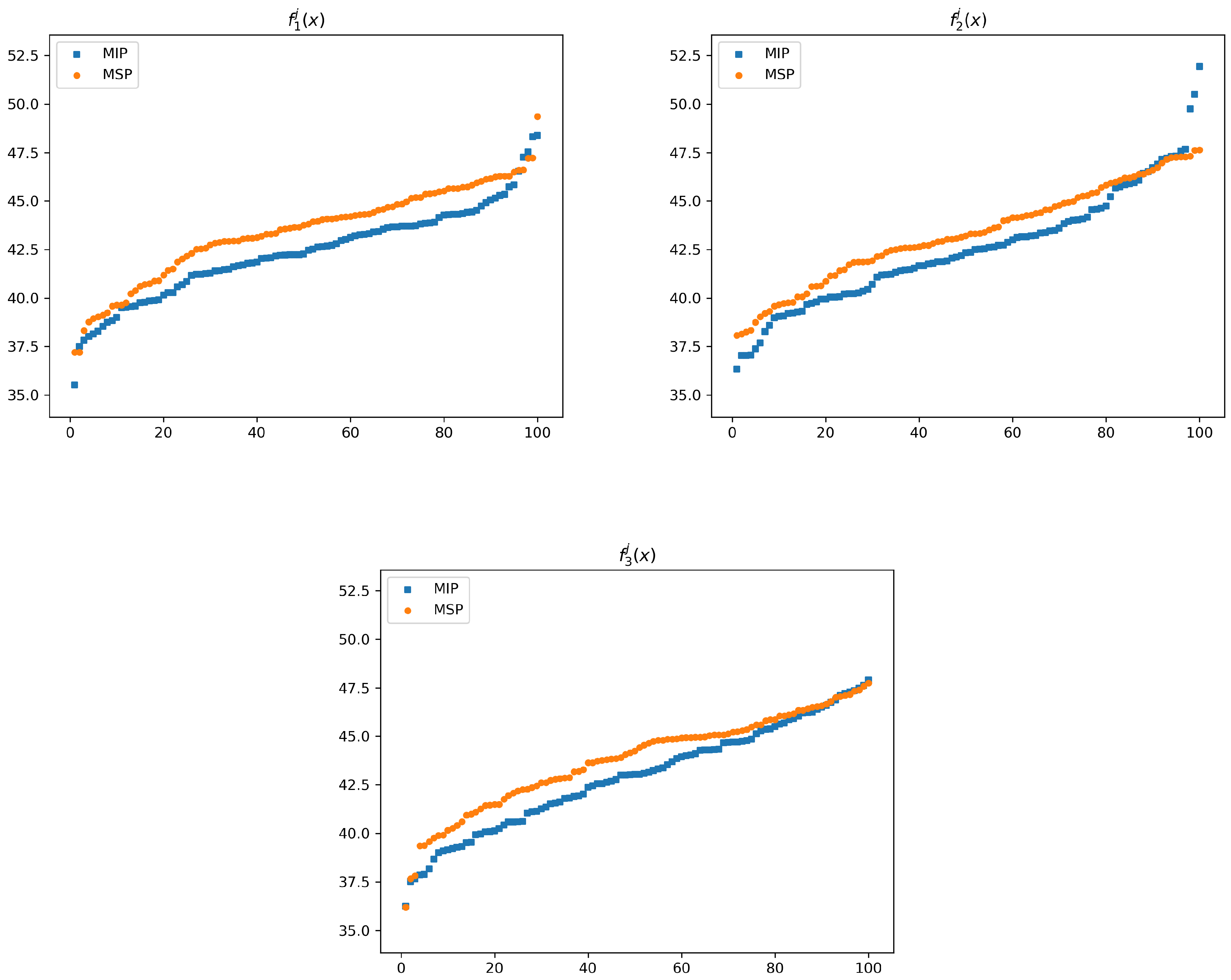
• $t_{\mathrm{MSP}},t_{\mathrm{MIP}}$: solution time in seconds of models (MSP) and (MIP). With them, the following value is calculated:

  $${\Delta }_{\mathrm{time}}:=\frac{t_{\mathrm{MSP}}}{t_{\mathrm{MIP}}}(time penalty factor)$$
  ${\Delta }_{\mathrm{time}}$, the time penalty factor, indicates the increase of computing time when solving model (MSP) rather than model (MIP).
• $z_{\mathrm{MSP}}^{*},z_{\mathrm{MIP}}^{*}$: optimal values of the models.
• $f_{\mathrm{MSP}}\left(x_{\mathrm{MIP}}^{*}\right),f_{\mathrm{MIP}}\left(x_{\mathrm{MSP}}^{*}\right)$: objective value of $x_{\mathrm{MIP}}^{*}$ in model (MSP) and vice versa.
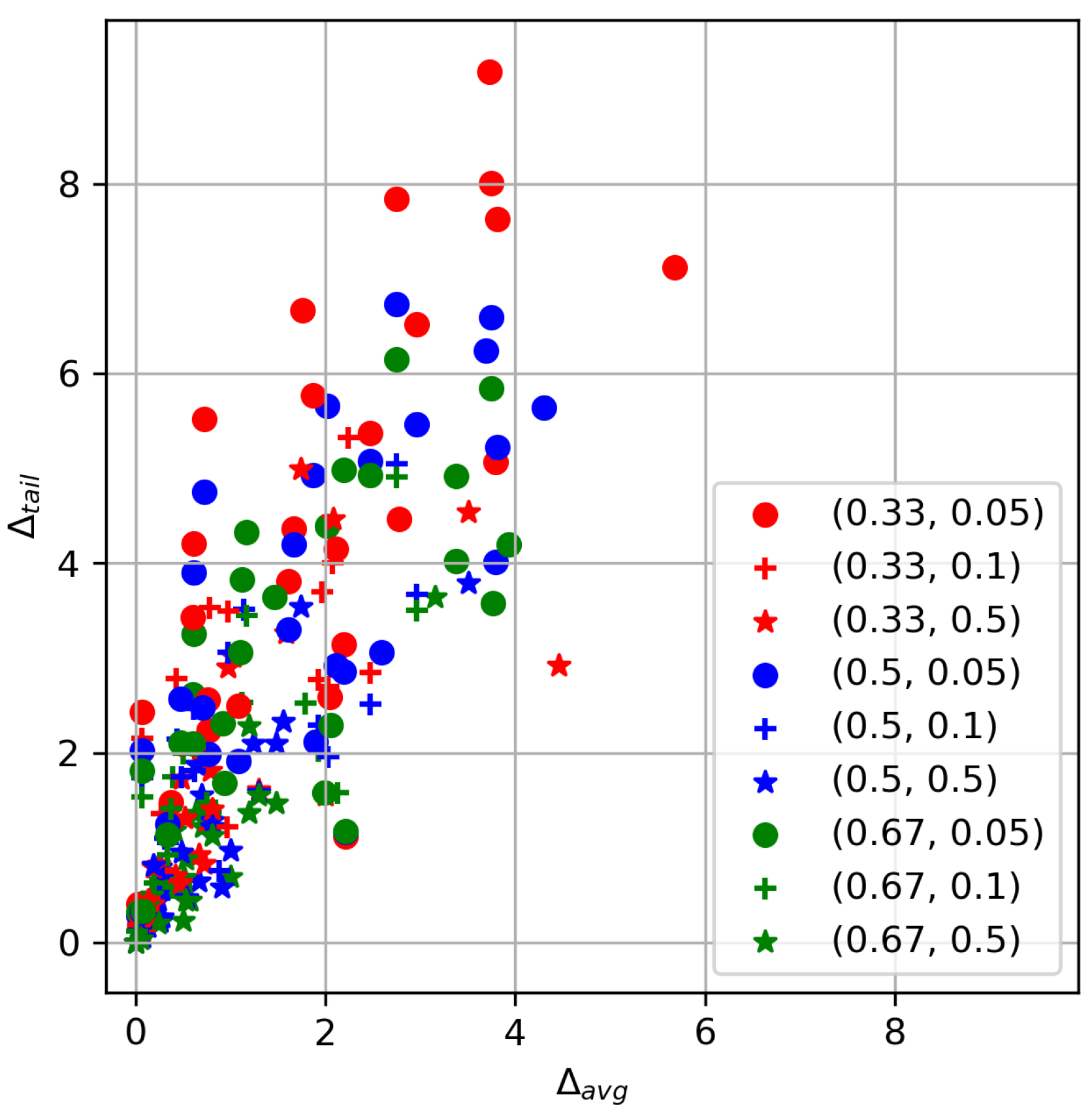
• To grasp the difference between the MSP and the naive approach, the following will be calculated:

  $$\begin{array}{cc}\hfill {\Delta }_{\mathrm{avg}}& :=100\frac{f_{\mathrm{MIP}}\left(x_{\mathrm{MSP}}^{*}\right)-z_{\mathrm{MIP}}^{*}}{z_{\mathrm{MIP}}^{*}}(deteriorating rate)\hfill \\ \hfill {\Delta }_{\mathrm{tail}}& :=100\frac{f_{\mathrm{MSP}}\left(x_{\mathrm{MIP}}^{*}\right)-z_{\mathrm{MSP}}^{*}}{f_{\mathrm{MSP}}\left(x_{\mathrm{MIP}}^{*}\right)}(improvement rate)\hfill \end{array}$$
  These quantities reflect what is the effect of making decision $x_{\mathrm{MSP}}^{*}$ instead of $x_{\mathrm{MIP}}^{*}$. Large values of ${\Delta }_{\mathrm{avg}}$ indicate high penalties for making decision $x_{\mathrm{MSP}}^{*}$ instead of $x_{\mathrm{MIP}}^{*}$ in average scenarios-criteria. Similarly, the larger ${\Delta }_{\mathrm{tail}}$, the higher benefit obtained from making decision $x_{\mathrm{MSP}}^{*}$ in tail events. They will be, respectively, called deteriorating rate and improvement rate.

The models are solved in GAMS 26.1.0 with solver IBM ILOG CPLEX 12.8.0.0, while using a personal computer with an Intel Core i7 processor and 16GB RAM.

• Experiment 1

The first experiment will consist on a full factorial design, in which the values of $\left|I\right|,\left|J\right|,\left|K\right|,r,\beta$ fall in these sets:

• $\left|I\right|\in \{50,100,200\}$
• $\left|J\right|\in \{5,25,100\}$
• $\left|K\right|\in \{3,6,9\}$
• $r\in \{0.33,0.5,0.67\}$
• $\beta \in \{0.05,0.1,0.5\}$

For each tuple $(I,J,K)$ a random instance will be generated using Algorithm 1, which will then be solved for every pair $(r,\beta )$. All of the criteria and scenarios are given the same importance and probabilities. That is, $w_k=\frac{1}{\left|K\right|}$, ${\pi }_j=\frac{1}{\left|J\right|}$. The time limit was set in two hours by instance, in which all but three of the $3^5=243$ configurations were solved to optimality.

• Experiment 2

For the next experiment, 100 random instances will be created, keeping the values of $\left|I\right|,\left|J\right|,\left|K\right|,r,\beta$ constant and equal to the median value of the previous experiment. That is, $\left|I\right|=100,\left|J\right|=25,\left|K\right|=6,r=0.5,\beta =0.1$. All of the criteria and scenarios are given the same importance and probabilities. All 100 instances were solved to optimality.

5.2. Results

• Experiment 1

Table A4. All instances of first experiment. The three instances with 200 objects, 100 scenarios, 6 criteria and $\beta =0.05$ did not reach the optimal solution in 2 h. The integrality gaps of the solution shown are $0.31\%,0.24\%$ and $0.19\%$ for $r=0.33,0.5$ and $0.67$ respectively.

$\mathit{\beta }\to$			0.05												0.1												0.5
$\mathit{r}\to$			0.33				0.5				0.67				0.33				0.5				0.67				0.33				0.5				0.67
|I|	|J|	|K|	${\mathit{t}}_{\mathbf{MSP}}$	${\mathit{t}}_{\mathbf{MIP}}$	${\Delta }_{\mathbf{avg}}$	${\Delta }_{\mathbf{tail}}$	${\mathit{t}}_{\mathbf{MSP}}$	${\mathit{t}}_{\mathbf{MIP}}$	${\Delta }_{\mathbf{avg}}$	${\Delta }_{\mathbf{tail}}$	${\mathit{t}}_{\mathbf{MSP}}$	${\mathit{t}}_{\mathbf{MIP}}$	${\Delta }_{\mathbf{avg}}$	${\Delta }_{\mathbf{tail}}$	${\mathit{t}}_{\mathbf{MSP}}$	${\mathit{t}}_{\mathbf{MIP}}$	${\Delta }_{\mathbf{avg}}$	${\Delta }_{\mathbf{tail}}$	${\mathit{t}}_{\mathbf{MSP}}$	${\mathit{t}}_{\mathbf{MIP}}$	${\Delta }_{\mathbf{avg}}$	${\Delta }_{\mathbf{tail}}$	${\mathit{t}}_{\mathbf{MSP}}$	${\mathit{t}}_{\mathbf{MIP}}$	${\Delta }_{\mathbf{avg}}$	${\Delta }_{\mathbf{tail}}$	${\mathit{t}}_{\mathbf{MSP}}$	${\mathit{t}}_{\mathbf{MIP}}$	${\Delta }_{\mathbf{avg}}$	${\Delta }_{\mathbf{tail}}$	${\mathit{t}}_{\mathbf{MSP}}$	${\mathit{t}}_{\mathbf{MIP}}$	${\Delta }_{\mathbf{avg}}$	${\Delta }_{\mathbf{tail}}$	${\mathit{t}}_{\mathbf{MSP}}$	${\mathit{t}}_{\mathbf{MIP}}$	${\Delta }_{\mathbf{avg}}$	${\Delta }_{\mathbf{tail}}$
50	5	3	0.12	0.13	3.75	8.01	0.15	0.12	3.75	8.01	0.18	0.14	3.51	4.54	0.14	0.14	3.75	6.59	0.12	0.12	3.75	6.59	0.20	0.17	3.51	3.79	0.12	0.12	3.75	5.84	0.12	0.12	3.75	5.84	0.13	0.12	3.16	3.64
		6	0.22	0.11	3.79	5.07	0.25	0.11	3.79	5.07	0.18	0.11	1.03	3.01	0.30	0.13	3.79	4.01	0.25	0.13	3.79	4.01	0.23	0.15	1.48	2.10	0.23	0.16	3.77	3.58	0.23	0.14	3.77	3.58	0.18	0.17	1.48	1.47
		9	0.28	0.14	1.76	6.67	0.36	0.14	1.76	6.67	0.20	0.15	1.58	3.26	0.22	0.14	2.02	5.66	0.21	0.14	2.02	5.66	0.22	0.14	1.24	2.10	0.20	0.15	2.02	4.39	0.22	0.13	2.02	4.39	0.25	0.15	1.20	1.37
	25	3	0.76	0.18	2.47	5.37	0.66	0.17	2.47	2.85	0.26	0.17	2.00	1.55	0.64	0.18	2.47	5.08	0.62	0.16	2.47	2.51	0.25	0.15	1.00	0.97	0.60	0.17	2.47	4.93	0.51	0.16	1.79	2.52	0.26	0.14	1.00	0.69
		6	1.20	0.16	1.87	5.77	0.91	0.29	1.96	3.70	0.49	0.18	0.79	1.81	1.15	0.18	1.87	4.93	0.74	0.18	1.14	3.51	0.41	0.18	0.70	1.55	0.93	0.16	1.17	4.33	0.78	0.18	1.17	3.45	0.38	0.16	0.71	1.22
		9	0.69	0.16	0.61	4.21	0.78	0.16	0.43	2.78	0.57	0.16	0.67	0.92	0.52	0.15	0.61	3.90	0.96	0.16	0.44	2.14	0.61	0.16	0.67	0.65	0.69	0.15	0.61	3.25	1.02	0.18	0.39	1.75	0.47	0.18	0.51	0.68
	100	3	1.15	0.15	0.07	2.43	0.78	0.15	0.07	2.15	0.44	0.14	0.07	0.16	1.07	0.14	0.07	2.02	0.83	0.19	0.07	1.74	0.34	0.14	0.07	0.16	1.14	0.15	0.07	1.81	0.85	0.16	0.07	1.53	0.36	0.14	0.07	0.14
		6	2.51	0.20	0.77	2.24	4.45	0.22	0.78	1.19	3.52	0.20	0.23	0.47	2.62	0.25	0.77	1.99	5.09	0.18	0.31	1.10	5.45	0.20	0.19	0.29	2.70	0.22	0.77	1.38	3.31	0.19	0.47	0.63	5.59	0.19	0.23	0.27
		9	4.06	0.18	0.03	0.41	1.47	0.17	0.03	0.30	1.07	0.16	0.00	0.00	2.75	0.17	0.03	0.29	1.12	0.16	0.03	0.30	1.11	0.16	0.00	0.00	2.06	0.19	0.03	0.32	1.10	0.16	0.03	0.18	1.16	0.17	0.00	0.00
100	5	3	1.24	0.26	3.81	7.63	1.29	0.20	3.81	7.63	0.37	0.22	2.08	4.47	0.72	0.18	3.81	5.22	0.66	0.18	3.81	5.22	0.32	0.27	1.56	2.33	0.74	0.19	3.38	4.02	1.13	0.23	3.38	4.02	0.28	0.20	0.63	1.36
		6	8.68	0.22	5.68	7.12	8.69	0.19	5.68	7.12	0.43	0.17	4.46	2.92	0.65	0.20	4.30	5.64	1.06	0.19	4.30	5.64	0.35	0.17	0.81	1.28	1.18	0.22	3.93	4.20	0.64	0.18	3.93	4.20	0.28	0.18	0.53	0.88
		9	3.31	0.18	2.19	3.14	3.26	0.20	2.19	3.14	0.67	0.18	0.97	2.90	1.04	0.20	2.19	2.86	0.96	0.20	2.19	2.86	0.23	0.14	0.64	1.88	1.02	0.17	0.92	2.31	0.90	0.17	0.92	2.31	0.24	0.18	0.41	1.18
	25	3	10.65	0.17	2.96	6.52	3.39	0.18	2.07	4.00	0.29	0.15	0.48	1.73	7.09	0.18	2.96	5.46	1.83	0.19	2.96	3.67	0.30	0.14	0.48	0.95	3.46	0.19	2.19	4.98	1.30	0.16	2.96	3.50	0.34	0.16	0.41	0.59
		6	32.12	0.20	2.78	4.47	9.18	0.19	0.78	3.53	0.44	0.18	0.52	1.31	26.53	0.18	2.59	3.06	3.64	0.22	0.61	2.47	0.32	0.15	0.26	0.79	12.77	0.17	0.60	2.62	0.90	0.17	0.50	2.00	0.41	0.17	0.26	0.65
		9	8.58	0.18	0.72	5.52	1.90	0.17	0.97	3.49	0.42	0.18	0.24	0.82	6.32	0.19	0.72	4.75	1.24	0.16	0.97	3.06	0.51	0.20	0.24	0.44	1.60	0.19	1.12	3.83	0.88	0.19	1.12	2.53	0.59	0.17	0.50	0.23
	100	3	51.23	0.22	2.21	1.12	1.67	0.21	0.27	1.36	0.82	0.18	0.09	0.25	22.70	0.21	2.21	1.16	1.22	0.19	0.34	1.05	0.81	0.18	0.05	0.17	18.75	0.16	2.21	1.17	0.84	0.22	0.34	0.92	0.75	0.18	0.05	0.13
		6	48.25	0.18	0.76	2.56	31.87	0.17	0.62	2.05	62.14	0.15	0.42	0.70	24.73	0.18	0.71	2.48	27.08	0.18	0.62	1.81	42.18	0.19	0.28	0.55	20.26	0.17	0.60	2.10	22.09	0.20	0.75	1.48	7.79	0.20	0.17	0.50
		9	2.16	0.19	0.37	1.48	3.34	0.18	0.29	0.77	1.84	0.17	0.18	0.41	1.80	0.17	0.34	1.25	2.87	0.20	0.28	0.69	2.22	0.19	0.26	0.22	1.67	0.18	0.34	1.14	2.77	0.19	0.20	0.63	3.09	0.16	0.08	0.13
200	5	3	146.24	0.23	1.61	3.81	140.12	0.20	1.61	3.81	7.71	0.23	1.30	1.61	151.22	0.21	1.61	3.30	135.09	0.24	1.61	3.30	4.60	0.21	1.30	1.58	83.44	0.22	1.10	3.06	89.20	0.21	1.10	3.06	4.21	0.22	1.30	1.55
		6	88.70	0.19	1.08	2.50	89.69	0.19	1.08	2.50	5.14	0.17	0.72	0.83	96.44	0.19	1.08	1.91	91.66	0.18	1.08	1.91	2.93	0.18	0.91	0.58	39.26	0.18	0.94	1.68	32.92	0.18	0.94	1.68	0.70	0.17	0.58	0.44
		9	468.37	0.15	3.73	9.18	484.89	0.14	3.73	9.18	29.46	0.16	1.74	4.99	304.04	0.16	3.69	6.24	305.90	0.16	3.69	6.24	2.71	0.16	1.74	3.54	110.03	0.15	3.38	4.92	107.34	0.14	3.38	4.92	0.91	0.17	1.20	2.28
	25	3	5629.58	0.33	2.75	7.84	4765.42	0.24	2.24	5.33	4.86	0.24	0.81	1.40	5430.90	0.25	2.75	6.73	3394.56	0.24	2.75	5.05	5.32	0.28	0.81	1.22	6896.05	0.25	2.75	6.15	2546.43	0.21	2.75	4.91	5.66	0.34	0.81	1.13
		6	2886.13	0.19	1.67	4.36	146.48	0.17	1.93	2.77	0.57	0.17	0.19	0.79	1651.91	0.21	1.67	4.20	15.06	0.22	1.93	2.29	0.71	0.21	0.19	0.81	93.66	0.19	1.46	3.64	19.36	0.19	1.93	2.02	0.55	0.18	0.12	0.40
		9	1235.12	0.32	2.05	2.59	342.32	0.22	0.96	1.22	1.99	0.21	0.22	0.26	404.70	0.29	1.90	2.12	28.09	0.21	0.88	0.76	0.82	0.20	0.13	0.17	99.73	0.21	1.99	1.58	2.23	0.22	0.39	0.58	0.87	0.20	0.06	0.08
	100	3	703.05	0.23	2.11	4.15	373.65	0.22	2.03	2.70	1.42	0.22	0.47	0.63	731.09	0.22	2.11	2.92	157.29	0.20	2.03	1.96	1.11	0.22	0.54	0.47	596.88	0.27	2.06	2.29	349.78	0.30	2.13	1.58	3.22	0.29	0.53	0.44
		6	7222.95	0.22	0.60	3.43	1814.25	0.18	0.48	2.08	22.11	0.21	0.13	0.44	7217.64	0.14	0.47	2.57	916.42	0.21	0.48	1.75	7.04	0.24	0.28	0.27	7216.94	0.15	0.47	2.11	656.48	0.20	0.37	1.41	7.89	0.22	0.24	0.20
		9	3321.23	0.34	0.07	0.28	16.40	0.20	0.02	0.18	2.33	0.17	0.08	0.08	198.14	0.19	0.07	0.32	14.84	0.21	0.02	0.13	2.31	0.21	0.08	0.05	47.16	0.23	0.08	0.33	9.77	0.21	0.01	0.12	2.63	0.20	0.06	0.04

(in the Appendix A) shows, for each of the 243 instances, the solution times of the MSP and the MIP models, and the deteriorating and improvement rates of using the MSP solution instead of the MIP solutions (measured in deviation to MIP solution).

Table 7. Objective values by scenario-criterion of solutions obtained with the multiobjective stochastic programming problem (MSP) and MIP models, for the first instance of the first experiment.

(a) MSP Solution				(b) MIP Solution
	$k_1$	$k_2$	$k_3$		$k_1$	$k_2$	$k_3$
$j_1$	11.97	11.26	11.00	$j_1$	9.65	10.75	9.71
$j_2$	11.96	9.92	13.71	$j_2$	11.19	10.17	14.90
$j_3$	13.48	13.51	10.92	$j_3$	14.05	13.55	9.40
$j_4$	13.62	13.13	13.71	$j_4$	14.12	13.00	13.35
$j_5$	12.94	11.35	13.47	$j_5$	13.64	10.33	11.42

shows the objective values, by scenario and criterion, of the first instance of the experiment. Such an instance contains 50 objects, five scenarios, three criteria, and the parameters r and $\beta$ are set to 0.33 and 0.05 respectively. Results show that the MSP solution (Table 7a) is more balanced through every scenario and criterion, with a worst value of 13.71. On the other hand, the MIP solution (Table 7b) attains larger (worse) values on some scenarios and criteria.

Table 8. Correlations.

	|I|	|J|	|K|	r	$\mathit{\beta }$
$t_{\mathrm{MSP}}$	0.34	0.09	−0.11	−0.05	−0.19
$t_{\mathrm{MIP}}$	0.51	0.18	−0.14	−0.03	−0.07
${\Delta }_{\mathrm{time}}$	0.31	0.11	−0.08	−0.02	−0.18
${\Delta }_{\mathrm{avg}}$	−0.05	−0.57	−0.28	−0.09	−0.36
${\Delta }_{\mathrm{tail}}$	−0.07	−0.56	−0.18	−0.21	−0.50

shows the correlations between the times and rates with the parameters of the instance. It can be seen how the MSP solution has a higher impact when fewer scenarios are considered. In addition to that, it can be appreciated that the MSP solution times decrease when $\beta$ increase, which is, when more scenarios are included in the $\beta$-average computation.

This observation is confirmed by

Table 9. MSP runtimes and increases as compared to MIP runtimes, grouped by $\beta$.

$\mathit{\beta }$	${\mathit{t}}_{\mathbf{MSP}}$					${\mathbf{\Delta }}_{\mathbf{time}}$
	Min	Mean	Median	Max	Std	Min	Mean	Median	Max	Std
0.05	0.12	659.49	6.32	7222.95	1787.07	0.94	3188.96	32.77	50473.04	9472.55
0.10	0.12	212.47	2.23	4765.42	728.49	0.98	1002.35	11.09	20192.48	3245.85
0.50	0.13	3.49	0.67	62.14	9.05	1.06	19.14	3.75	414.29	55.51

, in which it can be seen that the median time penalty factor (how much longer does it take to solve the MSP model than the MIP model) is much smaller when $\beta =0.5$ than when $\beta =0.05$.

The solution times of the MSP model are alarmingly high for some instances, due to the fact that the admissible integrality gap has been set to zero. If that is relaxed, it can be seen that all of the 243 instances reach an integrality gap smaller than 5% in about three seconds, 2% in about five seconds and 1% in about 88 seconds.

Table 10. Values of ${\Delta }_{\mathrm{avg}}$ and ${\Delta }_{\mathrm{tail}}$, grouped by r and $\beta$.

r	$\mathit{\beta }$	${\mathbf{\Delta }}_{\mathbf{avg}}$					${\mathbf{\Delta }}_{\mathbf{tail}}$
		Min	Mean	Median	Max	Std	Min	Mean	Median	Max	Std
0.33	0.05	0.03	1.94	1.87	5.68	1.42	0.28	4.37	4.21	9.18	2.43
	0.10	0.02	1.70	1.61	5.68	1.44	0.18	3.54	2.85	9.18	2.42
	0.50	0.00	0.93	0.52	4.46	1.08	0.00	1.57	0.92	4.99	1.46
0.50	0.05	0.03	1.87	1.90	4.30	1.30	0.29	3.58	3.30	6.73	1.89
	0.10	0.02	1.65	1.14	4.30	1.37	0.13	2.87	2.47	6.59	1.86
	0.50	0.00	0.72	0.54	3.51	0.75	0.00	1.07	0.79	3.79	1.01
0.67	0.05	0.03	1.64	1.17	3.93	1.24	0.32	3.04	3.06	6.15	1.62
	0.10	0.01	1.50	1.10	3.93	1.31	0.12	2.43	2.02	5.84	1.58
	0.50	0.00	0.60	0.50	3.16	0.66	0.00	0.80	0.59	3.64	0.81

groups instances by r and $\beta$, and shows the deteriorating and improvement rates. It can be seen that the improvement rate (in the tail) is generally higher than the deteriorating rate (in the average), especially in cases with small r and $\beta$.

This claim is also supported with Figure 2, where each of the 243 instances is shown according to the values of ${\Delta }_{\mathrm{avg}}$ and ${\Delta }_{\mathrm{tail}}$, and are grouped by the values of $(r,\beta )$. Almost all of the instances are above the imaginary line ${\Delta }_{\mathrm{avg}}={\Delta }_{\mathrm{tail}}$, which shows that considering the MSP solution improves in the tail more than it loses in the average situations. In addition to that, it can be seen that the largest improvements in the tail are on instances with $\beta =0.05$ (one of the usual values taken for CVaR), and especially with the smallest values of r. When r and $\beta$ grow, the differences between the MIP and MSP solutions are reduced.

Finally, Figure 3 shows the values of $f_k^j(x)$, where $x=x_{\mathrm{MIP}}^{*}$ in blue squares and $x=x_{\mathrm{MSP}}^{*}$ in orange circles, for just one of the created instances: 200 objects, 100 scenarios, three criteria, $r=0.33$, $\beta =0.05$. The values of $f_k^j(x)$ are represented for each criterion, sorting the scenarios from most to least favourable. It can be appreciated how $x_{\mathrm{MIP}}^{*}$ performs better than $x_{\mathrm{MSP}}^{*}$ in average criteria-scenarios, on the central part of the images; but, $x_{\mathrm{MSP}}^{*}$ is better with unfavourable situations, those with higher values of $f_k^j(x)$. This can be especially appreciated for the second criterion, in which there are three scenarios with objective values of $x_{\mathrm{MIP}}^{*}$ out of control.

• Experiment 2

Table A5. All instances of second experiment. $\left|I\right|=100,\left|J\right|=25,\left|K\right|=6,r=0.5,\beta =0.1$.

${\mathit{t}}_{\mathbf{MSP}}$	${\mathit{t}}_{\mathbf{MIP}}$	${\mathbf{\Delta }}_{\mathbf{avg}}$	${\mathbf{\Delta }}_{\mathbf{tail}}$	${\mathit{t}}_{\mathbf{MSP}}$	${\mathit{t}}_{\mathbf{MIP}}$	${\mathbf{\Delta }}_{\mathbf{avg}}$	${\mathbf{\Delta }}_{\mathbf{tail}}$
31.15	0.23	1.53	3.20	2.15	0.16	2.24	2.09
1.92	0.21	1.66	6.17	20.09	0.16	1.80	6.14
8.75	0.24	0.52	3.07	7.18	0.16	2.13	1.93
28.06	0.23	5.08	2.86	1.02	0.16	3.03	3.61
1.36	0.30	1.00	1.80	3.58	0.24	1.81	6.12
3.67	0.20	2.27	2.50	3.64	0.19	1.19	3.07
2.00	0.20	2.51	2.03	128.69	0.23	3.27	2.98
192.11	0.16	2.61	8.23	0.89	0.18	1.45	0.93
0.94	0.20	0.43	2.23	1.62	0.23	1.85	3.56
0.80	0.18	1.64	2.55	4.19	0.22	2.10	1.97
16.40	0.19	2.23	2.45	2.16	0.19	0.16	1.46
1.21	0.18	2.82	1.50	1.46	0.24	2.48	2.00
1.79	0.20	0.72	2.77	0.69	0.20	1.79	2.54
21.78	0.21	4.50	4.61	20.73	0.20	2.26	3.50
1.35	0.19	0.69	0.86	1.86	0.24	1.77	2.63
31.11	0.19	0.98	3.21	14.92	0.17	1.99	8.57
8.44	0.19	1.82	3.81	0.78	0.20	0.85	1.92
1.75	0.21	0.88	0.92	10.48	0.23	2.50	2.29
1.94	0.21	2.18	2.65	1.63	0.24	2.08	2.29
0.98	0.20	0.87	3.27	10.78	0.18	0.34	1.80
27.72	0.22	2.03	5.20	38.80	0.20	1.96	4.69
14.72	0.15	3.34	0.99	19.74	0.24	0.65	2.20
0.67	0.24	0.81	2.69	1.37	0.30	2.82	2.92
3.54	0.20	2.64	2.75	6.28	0.19	2.02	2.08
6.37	0.21	2.79	6.35	22.27	0.34	1.91	3.13
1.86	0.23	0.93	2.09	1.69	0.20	2.21	2.42
1.54	0.20	2.00	3.45	27.77	0.19	0.76	3.28
40.16	0.17	2.06	3.44	2.00	0.21	2.57	1.93
7.23	0.21	3.17	3.17	2.61	0.18	2.14	3.33
5.77	0.17	2.84	1.98	40.93	0.18	1.53	4.61
2.10	0.19	1.39	3.00	18.84	0.16	0.89	4.37
404.70	0.19	1.50	2.82	11.26	0.16	3.98	4.76
24.26	0.18	4.81	3.42	14.41	0.18	1.82	5.87
0.76	0.20	1.28	3.88	12.14	0.16	2.75	2.75
0.64	0.20	0.87	1.39	12.58	0.17	1.42	3.46
0.97	0.23	1.77	2.19	0.84	0.18	0.41	2.15
0.53	0.18	1.95	2.04	5.20	0.19	3.80	2.02
7.24	0.22	2.21	1.68	28.16	0.15	4.68	3.56
0.87	0.25	0.71	1.42	39.10	0.16	3.47	3.59
8.51	0.20	2.48	4.06	19.22	0.16	3.78	3.13
13.06	0.20	4.44	2.80	0.56	0.20	0.63	3.22
59.78	0.20	5.67	4.91	0.68	0.17	1.92	2.44
67.50	0.19	2.96	3.02	0.70	0.17	1.86	1.40
3.80	0.17	0.79	1.20	15.20	0.17	0.78	2.66
3.25	0.20	2.24	1.57	0.88	0.17	2.31	2.13
5.23	0.16	1.14	4.91	0.59	0.15	1.78	1.68
0.71	0.17	0.89	3.01	1.08	0.20	2.21	3.14
4.19	0.17	3.09	2.32	1.14	0.17	0.76	2.48
3.53	0.18	1.37	6.33	1.58	0.19	1.45	3.14
19.99	0.14	3.48	5.05	13.48	0.18	1.71	5.41

(in the appendix) contains the results for each of the 100 instances, all of them with constant parameters $\left|I\right|=100,\left|J\right|=25,\left|K\right|=6,r=0.5,\beta =0.1$.

Table 11. Summary of experiment 2.

	${\mathit{t}}_{\mathbf{MSP}}$	${\mathit{t}}_{\mathbf{MIP}}$	${\mathbf{\Delta }}_{\mathbf{time}}$	${\mathbf{\Delta }}_{\mathbf{avg}}$	${\mathbf{\Delta }}_{\mathbf{tail}}$
mean	16.98	0.20	91.31	2.03	3.09
std	46.57	0.03	254.68	1.12	1.49
min	0.53	0.14	2.81	0.16	0.86
25%	1.37	0.17	6.73	1.18	2.09
50%	3.74	0.19	19.72	1.93	2.81
75%	15.50	0.21	86.19	2.52	3.51
max	404.70	0.34	2175.82	5.67	8.57

contains a summary of the results, where it is again seen that the improvements in the tail are better than the loses in the average situations. Although single instances might take a long computing time, the median MSP solution time (3.74 s) is definitely satisfactory. It is worth mentioning that the models were implemented without providing any extra bounds or known cuts that could reduce the solution times.

6. Conclusions

In this paper, a new concept of solution has been proposed for Multiobjective Stochastic Programming problems, exploiting risk-aversion. The proposed concept combines the notions of conditional value-at-risk and ordered weighted averaging operator to find solutions protected against risks due to the uncertainty and under-achievement of criteria. Thus, this concept can be particularly useful in real-life situations, where there exists a great concern with respect to unfavourable situations, such as emergency management or portfolio optimization.

The solution concept is supported by an efficient way to compute it by a Mathematical Programming problem. This model is linear, provided that the underlying problem can be linearly representable. Numerical experiments have been conducted for validating this approach, solving a multiobjective stochastic knapsack problem.

The research has shown that the improvements in the tail (unfavourable situations) are consistently higher than loses on average situations, especially when small values of the parameters $\beta$ and r are chosen. These differences, although clearly noticeable, are not as high as one could expect. This is possibly due to the randomness of the data. It is reasonable to assume that, in actual real-life problems, there are choices that are more conservative for every scenario and criterion, and thus being preferable for risk-averse attitudes.

The results have shown that there is a clear increase in computational time as compared with risk neutral methods; however, this is arguably acceptable as a price to pay for being risk-averse. Furthermore, this could also be due to the random nature of the data. Nevertheless, it was also shown that allowing for even rather small integrality gaps (1%) leads to a drastic improvement in computing times.

References

1. Rommelfanger, H. The Advantages of Fuzzy Optimization Models in Practical Use. Fuzzy Optim. Decis. Mak. 2004, 3, 295–309. [Google Scholar] [CrossRef]
2. Gutjahr, W.; Nolz, P. Multicriteria optimization in humanitarian aid. Eur. J. Oper. Res. 2016, 252, 351–366. [Google Scholar] [CrossRef]
3. Ferrer, J.; Martín-Campo, F.; Ortuño, M.; Pedraza-Martínez, A.; Tirado, G.; Vitoriano, B. Multi-criteria optimization for last mile distribution of disaster relief aid: Test cases and applications. Eur. J. Oper. Res. 2018, 269, 501–515. [Google Scholar] [CrossRef]
4. Sun, G.; Zhang, H.; Fang, J.; Li, G.; Li, Q. A new multi-objective discrete robust optimization algorithm for engineering design. Appl. Math. Model. 2018, 53, 602–621. [Google Scholar] [CrossRef]
5. Karsu, Ö.; Morton, A. Inequity averse optimization in operational research. Eur. J. Oper. Res. 2015, 245, 343–359. [Google Scholar] [CrossRef] [Green Version]
6. Angilella, S.; Mazzù, S. The financing of innovative SMEs: A multicriteria credit rating model. Eur. J. Oper. Res. 2015, 244, 540–554. [Google Scholar] [CrossRef] [Green Version]
7. Fotakis, D. Multi-objective spatial forest planning using self-organization. Ecol. Inform. 2015, 29, 1–5. [Google Scholar] [CrossRef]
8. Guido, R.; Conforti, D. A hybrid genetic approach for solving an integrated multi-objective operating room planning and scheduling problem. Comput. Oper. Res. 2017, 87, 270–282. [Google Scholar] [CrossRef]
9. Eiselt, H.; Marianov, V. Location modeling for municipal solid waste facilities. Comput. Oper. Res. 2015, 62, 305–315. [Google Scholar] [CrossRef]
10. Liberatore, F.; Camacho-Collados, M. A Comparison of Local Search Methods for the Multicriteria Police Districting Problem on Graph. Math. Prob. Eng. 2016, 2016, 3690474. [Google Scholar] [CrossRef] [Green Version]
11. Bast, H.; Delling, D.; Goldberg, A.; Müller-Hannemann, M.; Pajor, T.; Sanders, P.; Wagner, D.; Werneck, R. Route planning in transportation networks. In Lecture Notes in Computer Science (Including Subseries Lecture Notes in Artificial Intelligence and Lecture Notes in Bioinformatics); Springer: Cham, Switzerland, 2016; pp. 19–80. [Google Scholar]
12. Samà, M.; Meloni, C.; D’Ariano, A.; Corman, F. A multi-criteria decision support methodology for real-time train scheduling. J. Rail Transp. Plan. Manag. 2015, 5, 146–162. [Google Scholar] [CrossRef]
13. Spina, L.; Scrivo, R.; Ventura, C.; Viglianisi, A. Urban renewal: Negotiation procedures and evaluation models. In Lecture Notes in Computer Science (Including Subseries Lecture Notes in Artificial Intelligence and Lecture Notes in Bioinformatics); Springer: Cham, Switzerland, 2015; pp. 88–103. [Google Scholar]
14. Carli, R.; Dotoli, M.; Pellegrino, R. A decision-making tool for energy efficiency optimization of street lighting. Comput. Oper. Res. 2018, 96, 223–235. [Google Scholar] [CrossRef]
15. Ehrgott, M. Multicriteria Optimization, 2nd ed.; Springer: Berlin/Heidelberg, Germay, 2005. [Google Scholar]
16. Birge, J.R.; Louveaux, F. Introduction to Stochastic Programming; Springer: New York, NY, USA, 2011. [Google Scholar]
17. Ben-Tal, A.; Nemirovski, A. Robust solutions of uncertain linear programs. Oper. Res. Lett. 1999, 25, 1–13. [Google Scholar] [CrossRef] [Green Version]
18. Chen, X.; Sim, M.; Sun, P. A Robust Optimization Perspective on Stochastic Programming. Oper. Res. 2007, 55, 1058–1071. [Google Scholar] [CrossRef]
19. Klamroth, K.; Köbis, E.; Schöbel, A.; Tammer, C. A unified approach to uncertain optimization. Eur. J. Oper. Res. 2017, 260, 403–420. [Google Scholar] [CrossRef]
20. Gabrel, V.; Murat, C.; Thiele, A. Recent advances in robust optimization: An overview. Eur. J. Oper. Res. 2014, 235, 471–483. [Google Scholar] [CrossRef]
21. Yao, H.; Li, Z.; Lai, Y. Mean–CVaR portfolio selection: A nonparametric estimation framework. Comput. Oper. Res. 2013, 40, 1014–1022. [Google Scholar] [CrossRef]
22. Mansini, R.; Ogryczak, W.; Speranza, M.G. Linear and Mixed Integer Programming for Portfolio Optimization; Springer International Publishing: Berlin/Heidelberg, Germany, 2015. [Google Scholar]
23. Liu, X.; Küçükyavuz, S.; Noyan, N. Robust multicriteria risk-averse stochastic programming models. Ann. Oper. Res. 2017, 259, 259–294. [Google Scholar] [CrossRef] [Green Version]
24. Dixit, V.; Tiwari, M.K. Project portfolio selection and scheduling optimization based on risk measure: A conditional value at risk approach. Ann. Oper. Res. 2020, 285, 9–33. [Google Scholar] [CrossRef]
25. Fernández, E.; Hinojosa, Y.; Puerto, J.; da Gama, F.S. New algorithmic framework for conditional value at risk: Application to stochastic fixed-charge transportation. Eur. J. Oper. Res. 2019, 277, 215–226. [Google Scholar] [CrossRef]
26. Rockafellar, R.; Uryasev, S. Conditional value-at-risk for general loss distributions. J. Bank. Financ. 2002, 26, 1443–1471. [Google Scholar] [CrossRef]
27. Goicoechea, A. Deterministic Equivalents for Use in Multiobjective, Stochastic Programming. IFAC Proc. Vol. 1980, 13, 31–40. [Google Scholar] [CrossRef]
28. Leclercq, J.P. Stochastic programming: An interactive multicriteria approach. Eur. J. Oper. Res. 1982, 10, 33–41. [Google Scholar] [CrossRef]
29. Caballero, R.; Cerdá, E.; Muñoz, M.M.; Rey, L. Stochastic approach versus multiobjective approach for obtaining efficient solutions in stochastic multiobjective programming problems. Eur. J. Oper. Res. 2004, 158, 633–648. [Google Scholar] [CrossRef] [Green Version]
30. Aouni, B.; Ben Abdelaziz, F.; Martel, J.M. Decision-maker’s preferences modeling in the stochastic goal programming. Eur. J. Oper. Res. 2005, 162, 610–618. [Google Scholar] [CrossRef]
31. Ben Abdelaziz, F.; Masri, H. A compromise solution for the multiobjective stochastic linear programming under partial uncertainty. Eur. J. Oper. Res. 2010, 202, 55–59. [Google Scholar] [CrossRef]
32. Ben Abdelaziz, F.; Aouni, B.; Fayedh, R.E. Multi-objective stochastic programming for portfolio selection. Eur. J. Oper. Res. 2007, 177, 1811–1823. [Google Scholar] [CrossRef]
33. Muñoz, M.M.; Luque, M.; Ruiz, F. INTEREST: A reference-point-based interactive procedure for stochastic multiobjective programming problems. OR Spectr. 2010, 32, 195–210. [Google Scholar] [CrossRef]
34. Ben Abdelaziz, F. Solution approaches for the multiobjective stochastic programming. Eur. J. Oper. Res. 2012, 216, 1–16. [Google Scholar] [CrossRef]
35. Gutjahr, W.J.; Pichler, A. Stochastic multi-objective optimization: A survey on non-scalarizing methods. Ann. Oper. Res. 2013, 236, 475–499. [Google Scholar] [CrossRef]
36. Engau, A.; Sigler, D. Pareto solutions in multicriteria optimization under uncertainty. Eur. J. Oper. Res. 2020, 281, 357–368. [Google Scholar] [CrossRef]
37. Álvarez-Miranda, E.; Garcia-Gonzalo, J.; Ulloa-Fierro, F.; Weintraub, A.; Barreiro, S. A multicriteria optimization model for sustainable forest management under climate change uncertainty: An application in Portugal. Eur. J. Oper. Res. 2018, 269, 79–98. [Google Scholar] [CrossRef]
38. Díaz-García, J.A.; Bashiri, M. Multiple response optimisation: An approach from multiobjective stochastic programming. Appl. Math. Model. 2014, 38, 2015–2027. [Google Scholar] [CrossRef]
39. Teghem, J.; Dufrane, D.; Thauvoye, M.; Kunsch, P. Strange: An interactive method for multi-objective linear programming under uncertainty. Eur. J. Oper. Res. 1986, 26, 65–82. [Google Scholar] [CrossRef]
40. Bath, S.K.; Dhillon, J.S.; Kothari, D.P. Stochastic Multi-Objective Generation Dispatch. Electr. Power Compon. Syst. 2004, 32, 1083–1103. [Google Scholar] [CrossRef]
41. Gazijahani, F.S.; Ravadanegh, S.N.; Salehi, J. Stochastic multi-objective model for optimal energy exchange optimization of networked microgrids with presence of renewable generation under risk-based strategies. ISA Trans. 2018, 73, 100–111. [Google Scholar] [CrossRef] [PubMed]
42. Claro, J.; De Sousa, J. A multiobjective metaheuristic for a mean-risk multistage capacity investment problem. J. Heurist. 2010, 16, 85–115. [Google Scholar] [CrossRef]
43. Manopiniwes, W.; Irohara, T. Stochastic optimisation model for integrated decisions on relief supply chains: Preparedness for disaster response. Int. J. Prod. Res. 2016, 55, 979–996. [Google Scholar] [CrossRef]
44. Bastian, N.; Griffin, P.; Spero, E.; Fulton, L. Multi-criteria logistics modeling for military humanitarian assistance and disaster relief aerial delivery operations. Optim. Lett. 2016, 10, 921–953. [Google Scholar] [CrossRef]
45. Şakar, C.T.; Köksalan, M. A stochastic programming approach to multicriteria portfolio optimization. J. Glob. Optim. 2012, 57, 299–314. [Google Scholar] [CrossRef]
46. Salas-Molina, F.; Rodriguez-Aguilar, J.A.; Pla-Santamaria, D. A stochastic goal programming model to derive stable cash management policies. J. Glob. Optim. 2020, 76, 333–346. [Google Scholar] [CrossRef]
47. Yager, R. On ordered weighted averaging aggregation operators in multicriteria decisionmaking. IEEE Trans. Syst. Man Cybern. 1988, 18, 183–190. [Google Scholar] [CrossRef]
48. Fernández, F.; Puerto, J. Análisis de sensibilidad de las soluciones del problema lineal múltiple ordenado. TOP 1992, 7, 17–29. [Google Scholar]
49. Nickel, S.; Puerto, J. A unified approach to network location problems. Networks 1999, 34, 283–290. [Google Scholar] [CrossRef]
50. Yager, R.R.; Alajlan, N. Some issues on the OWA aggregation with importance weighted arguments. Knowl. Based Syst. 2016, 100, 89–96. [Google Scholar] [CrossRef]
51. Puerto, J.; Rodríguez-Chía, A.M.; Tamir, A. Revisiting k-sum optimization. Math. Program. 2017, 165, 579–604. [Google Scholar] [CrossRef]
52. Kalcsics, J.; Nickel, S.; Puerto, J.; Tamir, A. Algorithmic results for ordered median problems. Oper. Res. Lett. 2002, 30, 149–158. [Google Scholar] [CrossRef]
53. Blanco, V.; Ali, S.E.H.B.; Puerto, J. Minimizing ordered weighted averaging of rational functions with applications to continuous location. Comput. Oper. Res. 2013, 40, 1448–1460. [Google Scholar] [CrossRef]
54. Blanco, V.; Puerto, J.; El Haj Ben Ali, S. Revisiting Several Problems and Algorithms in Continuous Location with τ Norms. Comput. Optim. Appl. 2014, 58, 563–595. [Google Scholar] [CrossRef]
55. Ponce, D.; Puerto, J.; Ricca, F.; Scozzari, A. Mathematical programming formulations for the efficient solution of the k-sum approval voting problem. Comput. Oper. Res. 2018, 98, 127–136. [Google Scholar] [CrossRef] [Green Version]
56. Filippi, C.; Ogryczak, W.; Speranza, M.G. Bridging k-sum and CVaR optimization in MILP. Comput. Oper. Res. 2019, 105, 156–166. [Google Scholar] [CrossRef]
57. Nickel, S.; Puerto, J. Location Theory; Springer: Berlin/Heidelberg, Germany, 2005. [Google Scholar]
58. Bilbao-Terol, A.; Arenas-Parra, M.; Cañal-Fernández, V. Selection of Socially Responsible Portfolios using Goal Programming and fuzzy technology. Inf. Sci. 2012, 189, 110–125. [Google Scholar] [CrossRef]
Figure 1. The results from illustrative example. (a) Optimal alternative for some values of r and β , where each of the four alternatives is colour-coded. (b) Optimal values of function h r β ( x ) for some values of r and β .
Mathematics 08 02026 g001
Figure 2. Values Δ avg and Δ tail for each of the 243 instances, grouped by values of ( r , β ) .
Mathematics 08 02026 g002
Figure 3. Single instance with 100 scenarios and three criteria. For each k, sorted values of f k j ( x ) , where x = x MIP * in blue squares and x = x MSP * in orange circles.
Mathematics 08 02026 g003