Solving Generalized Equations with Bounded Variables and Multiple Residuated Operators

Abstract

This paper studies the resolution of sup-inequalities and sup-equations with bounded variables such that the sup-composition is defined by using different residuated operators of a given distributive biresiduated multi-adjoint lattice. Specifically, this study has analytically determined the whole set of solutions of such sup-inequalities and sup-equations. Since the solvability of these equations depends on the character of the independent term, the resolution problem has been split into three parts distinguishing among the bottom element, join-irreducible elements and join-decomposable elements.

1. Introduction

The problem of solving equations with bounded variables and general/flexible operators is an interesting topic nowadays [1,2,3,4,5,6,7,8,9,10]. For example, these kinds of equations arise when imprecise data need to be modeled, such as trying to handle fuzzy sets. Lotfi A. Zadeh introduced fuzzy sets and fuzzy logic in the sixties [11] with the main goal of mathematically interpreting imprecise predicates—i.e., names of non-precisely determined classes of objects. This imprecision is usually modeled considering a degree (also called truth-value) between the two classical “falsum” (0) and “verum” (1) values for the properties describing every object. The possible set of truth-values ranges from the unit interval or some granularity of it (a finite subset) [12,13] to a general partially ordered set, such as a lattice or a multilattice [14,15,16].

One of the most studied theories based on fuzzy sets is fuzzy relation equations (FRE), which was introduced by E. Sanchez in the eighties [17]. The resolution of FRE arises naturally in problems associated with imprecise, incomplete and/or vague data, as J. A. Goguen explained in his seminal paper [18]:

“The importance of relations is almost self-evident. Science is, in a sense, the discovery of relations between observables … Difficulties arise in the so-called “soft” sciences because the relations involved do not appear to be “hard” as they are, say, in classical physics … We suggest that further difficulties might be cleared up through a systematic exploitation of fuzziness”.

From its introduction, this theory has been developed from both theoretical and applied points of view [19,20]. For example, Sanchez used FRE for medical diagnosis [21] and fuzzy control [19]. Besides, negations have recently been considered in FRE for modelling bipolar information [4,7,22,23], and applied to optimization problems [5,6], enterprise architecture [10,24], decision support [3], etc.

On the other hand, the multi-adjoint philosophy arose at the beginning of this century [25,26] as a general flexible mathematical framework based on adjustable robust operators, called adjoint pairs and triples. This philosophy has been applied to diverse theories, such as logic programming [27,28], formal concept analysis [15,29,30], rough set theory [31,32], fuzzy relation equations [33,34], mathematical morphology [1,9], etc. The resulting multi-adjoint settings are more flexible than the previous ones, reducing the requirements to be satisfied by the considered operators. In the particular framework of multi-adjoint FRE, Díaz-Moreno et al. introduced a novel relationship with the property-oriented and object-oriented concept lattices in [35], which provided, among other achievements, a characterization of the whole set of solutions of a multi-adjoint relation equation [36]. The computation of the covering problem has also been related to the resolution of FRE [8,37]. Moreover, the use of “dual” residuated implications was fundamental for analytically determining the minimal solutions of FRE [2,34,38].

The main goal of the current manuscript is to study the resolution of a primitive form of multi-adjoint FRE: multi-adjoint sup-equations. Namely, multi-adjoint FRE can be seen as systems of multi-adjoint sup-equations. Therefore, the investigation of such sup-equations is instrumental to comprehend and deepen into the nature of multi-adjoint FRE, thus leading to their resolution. To the best of our knowledge, Refs. [34,38] are the current papers with the most general frameworks in which the analytical expression of the minimal solutions of FRE are given. The author in [38] deals with equations defined from a triangular norm in a complete distributive lattice, providing their solution set, whilst [34] considers a general setting based on a sup-preserving conjunction, but all minimal solutions of the FRE are not characterized, in general.

Our approach is based on the point of view considered by B. De Baets in [38]. In this aforementioned paper, the following sup-equations

$$\underset{j\in \{1,\dots ,m\}}{\bigvee }{a}_j \& x_j=b\mathrm{and}\underset{j\in \{1,\dots ,m\}}{\bigvee }{x}_j \& a_j=b$$

as well as their corresponding sup-inequalities

$$\underset{j\in \{1,\dots ,m\}}{\bigvee }{a}_j \& x_j⪯b,\underset{j\in \{1,\dots ,m\}}{\bigvee }{x}_j \& a_j⪯b,\underset{j\in \{1,\dots ,m\}}{\bigvee }{a}_j \& x_j⪰b,\underset{j\in \{1,\dots ,m\}}{\bigvee }{x}_j \& a_j⪰b$$

were considered, where the conjunction & is a t-norm defined on a complete distributive lattice. Applying the philosophy of the multi-adjoint paradigm, we analyse the resolution of sup-equations and sup-inequalities allowing the use of different conjunctions of a given distributive biresiduated multi-adjoint lattice. The current contribution notably reduce the required properties of these conjunctions. In particular, neither commutativity nor associativity are required. Hence, the results shown here extend the work carried out in [38] in two ways. On the one hand, providing an extra grade of flexibility to the conjunctions in the algebraic framework, and on the other hand, allowing different conjunctions appearing in the same equation.

Focusing on the right-hand side of multi-adjoint sup-equations and sup-inequalities, the resolution strategy shown here differentiates among the bottom element, join-irreducible elements and join-decomposable elements, which are all possible kinds of elements in a lattice satisfying the descendent chain condition [39]. Hence, for all scenarios in these general kind of lattices, the whole solution set is analytically determined in this paper. Therefore, the solvability and the computation of the whole set of solutions of multi-adjoint sup-equations and sup-inequalities is characterized. Thus, the current manuscript significantly broadens the scope of the results presented in [34], fixing a general multi-adjoint framework where all minimal solutions are characterized. Moreover, from a theoretical perspective, this work may have a significant impact on the resolution of multi-adjoint relation equations, as well as on the study of bipolar fuzzy relation equations.

In what regards the applicative potential of the results, handling a general framework enables modelling a wide range of real problems. Furthermore, computing all solutions of a multi-adjoint sup-equation immediately sets an appealing starting point to develop real applications of this manuscript in fields such as forensics analysis, medical diagnosis and decision support, among others.

2. Preliminary Notions

The following notions and results aim to facilitate the comprehension of this paper. To begin with, some definitions related to lattice theory are shown below [39,40,41].

Definition 1.

Let $(L,⪯)$ be a partially ordered set (poset). We say that $(L,⪯)$ is a lattice if $x\vee y,x\wedge y\in L$ for all $x,y\in L$. Besides, if the supremum and the infimum of S exist for all $S\subseteq L$, then $(L,⪯)$ is called a complete lattice.

A lattice is said to be distributive when its inner operators, that is the join and the meet, distribute each other. In formal terms:

Definition 2.

A lattice $(L,⪯)$ is a distributive lattice if the following property holds, for all $x,y,z\in L$:

$$x\wedge (y\vee z)=(x\wedge y)\vee (x\wedge z)$$

A well-known characterization of distributive lattices is stated by the $M_3$–$N_5$ Theorem.

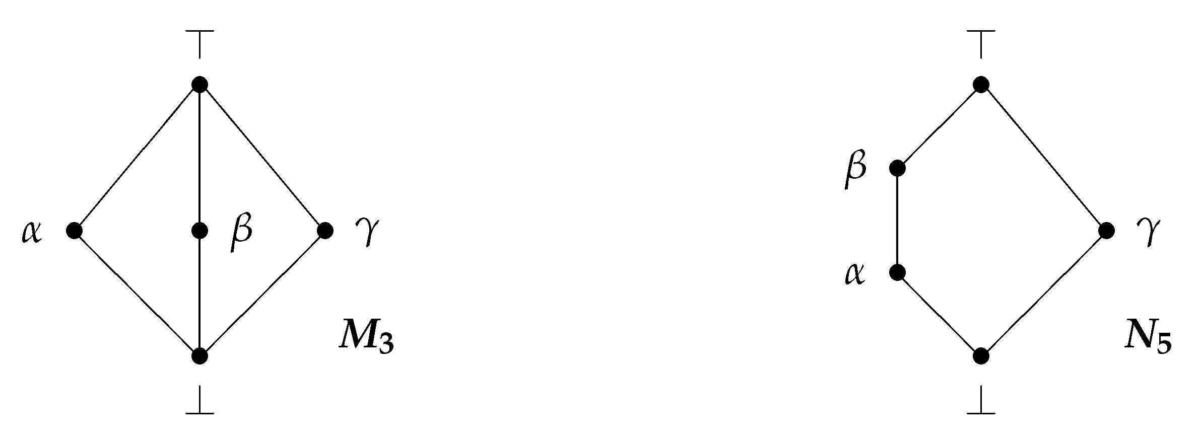
Theorem 1.

[41] A lattice $(L,⪯)$ is distributive if and only if neither $M_3$ nor $N_5$ is a sublattice of $(L,⪯)$, being $M_3$ and $N_5$ the lattices whose Hasse diagrams are given in Figure 1.

Since the current paper deals with the resolution of sup-equations, the lattice join operator plays a key role in its development. We will distinguish between the elements that can be written as the join of two other elements and the elements which cannot.

Definition 3.

Let $(L,⪯)$ be a lattice. An element $x\in L$ is said to be:

• Join-irreducible if $x\ne \perp$ and $x=a\vee b$ implies $x=a$ or $x=b$, for all $a,b\in L$.
• Join-reducible or join-decomposable if there exists a subset of join-irreducible elements $A\subseteq L$, with $\left|A\right|\ge 2$, such that $\bigvee A=x$. Besides, we say that A is a join-decomposition of x.

Notice that, all elements in a finite lattice are either join-irreducible or join-decomposable, except for the bottom element. This partition also arises in lattices satisfying the descendent chain condition (DCC) [39]. Another notion based on the join operator is given next.

Definition 4.

Let $(L,⪯)$ be a lattice. An element $x\in L$ is said to be join-prime if $x⪯y\vee z$ implies $x⪯y$ or $x⪯z$.

Clearly, all join-prime elements in a lattice are join-irreducible. Indeed, these two kind of elements coincide in distributive lattices. Furthermore, the following property holds for join-irreducible elements of a distributive lattice.

Proposition 1

([40]). Let $(L,⪯)$ be a distributive lattice and $b\in L$ a join-irreducible element. Given $a_1,\dots ,a_m\in L$, then $b⪯a_1\vee \cdots \vee a_m$ if and only if there exists $j\in \{1,\dots ,m\}$ such that $b⪯a_j$.

Lattice homomorphisms, as it name suggests, are mappings which preserve the lattice join and meet operators.

Definition 5.

Let $(L,⪯)$ be a lattice and $f:L\to L$ a mapping. We say that f is a lattice homomorphism, or simply a homomorphism, if $f(supA)=sup\left(f\right(A\left)\right)$ and $f(infA)=inf\left(f\right(A\left)\right)$, for each $A\in \mathcal{P}\left(L\right)\backslash \{⌀\}$.

The notion of lattice homomorphism can be naturally extended to mappings whose domain is $L^n$ as follows.

Definition 6.

Let $(L,⪯)$ be a lattice and $f:L^n\to L$ a mapping. We say that f is a lattice homomorphism, or simply a homomorphism, if the partial mappings of f are homomorphisms.

The classical notion of fuzzy implication is stated as a binary mapping ← that is order-preserving in the consequent and order-reversing in the antecedent. Unfortunately, as P. Hájek argued in [12], this definition is not powerful enough to model the modus ponens inference rule, which is the main deductive argument form in logic. To this aim, adjoint pairs were introduced in [25] as a couple of binary mappings $(\&,\leftarrow )$ representing a conjunction and an implication, respectively. It needs to be stressed that neither commutativity nor associativity are required on &. Indeed, if & is non-commutative, there are two ways to define ←. This fact gives rise to a more general definition than adjoint pairs, known as adjoint triple.

Definition 7

([42]). Let $(L,⪯)$ be a lattice. Given three mappings $\&,\swarrow ,\nwarrow :L\times L\to L$, we say that $(\&,\swarrow ,\nwarrow )$ is an adjoint triple with respect to L if the following double equivalence holds:

$$x⪯z\swarrow yifandonlyifx \& y⪯zifandonlyify⪯z\nwarrow x$$

The previous double equivalence is called adjoint property and the mappings $\swarrow ,\nwarrow$ are called the residuated implications of $\&$.

The proposition below shows some properties of adjoint triples. Among others, the form of the residuated implications of an adjoint triple is provided.

Proposition 2

([42,43]). Let $(L,⪯)$ be a complete lattice and $(\&,\swarrow ,\nwarrow )$ an adjoint triple with respect to L. The following statements hold:

1 

$\&$ is order-preserving on both arguments.

2 

↙ and ↖ are order-preserving on the first argument and order-reversing on the second argument.

3 

$(z\swarrow y) \& y⪯z$ for each $x,y,z\in L$.

4 

$x \& (z\nwarrow x)⪯z$ for each $x,y,z\in L$.

5 

$x \& \perp =\perp \& x=\perp$ for each $x\in L$.

6 

The residuated implications of $\&$ are unique, and they are defined as $z\swarrow y=max\{x\in L\mid x \& y⪯z\}$ and $z\nwarrow x=max\{y\in L\mid x \& y⪯z\}$.

A complete lattice endowed with a finite number of adjoint pairs is usually called multi-adjoint lattice. Similarly, a biresiduated multi-adjoint lattice was defined in [13] as a complete lattice enriched with a finite number of adjoint triples. In this paper, we will also require the boundary conditions with the top element of the lattice.

Definition 8.

The tuple $(L,⪯,{\&}_1,{\swarrow }^1,{\nwarrow }_1,\dots ,{\&}_n,{\swarrow }^{\kappa },{\nwarrow }_{\kappa })$ is a biresiduated multi-adjoint lattice if the following properties are verified:

• $(L,⪯)$ is a complete lattice.
• $({\&}_i,{\swarrow }^i,{\nwarrow }_i)$ is an adjoint triple, for each $i\in \{1,\dots ,\kappa \}$.
• ⊤ is the identity element of ${\&}_i$ for each $i\in \{1,\dots ,\kappa \}$, that is, $\top {\&}_i x=x {\&}_i \top =x$, for each $x\in L$.

Given a biresiduated multi-adjoint lattice $(L,⪯,{\&}_1,{\swarrow }^1,{\nwarrow }_1,\dots ,{\&}_{\kappa },{\swarrow }^{\kappa },{\nwarrow }_{\kappa })$, following the approach taken in [38], we will associate each ${\&}_i$ with two extra operators. Specifically, for each $i\in \{1,\dots ,\kappa \}$, we define the mappings $,{⤣}_i:L\times L\to L$ as:

(1)

Since $(L,⪯)$ is a complete lattice, the mappings $,{⤣}_i$ are well-defined. Clearly, both mappings coincide when ${\&}_i$ is a commutative operator, as well as ${\swarrow }^i$ and ${\nwarrow }_i$ coincide. Notice that, unlike the definition of ${\swarrow }^i$ and ${\nwarrow }_i$ as a maximum, and ${⤣}_i$ cannot be defined as the minimum of the sets $\{x\in L\mid z⪯x {\&}_i y\}$ and $\{y\in L\mid z⪯x {\&}_i y\}$, respectively, because these sets might be empty [34]. For instance, this occurs if $y\prec z$ or $x\prec z$, respectively.

3. Multi-Adjoint Sup-Inequalities and Sup-Equations

Let $(L,⪯,{\&}_1,{\swarrow }^1,{\nwarrow }_1,\dots ,{\&}_{\kappa },{\swarrow }^{\kappa },{\nwarrow }_{\kappa })$ be a biresiduated multi-adjoint lattice and $\sigma :\{1,\dots ,m\}\to \{1,\dots ,\kappa \}$ be a mapping which associates each index $j\in \{1,\dots ,m\}$ with some particular conjunction in the biresiduated multi-adjoint lattice. A multi-adjoint sup-equation is an expression of the form

$$\underset{j\in \{1,\dots ,m\}}{\bigvee }{a}_j {\&}_{\sigma \left(j\right)} x_j=b\mathrm{or}\underset{j\in \{1,\dots ,m\}}{\bigvee }{x}_j {\&}_{\sigma \left(j\right)} a_j=b$$

In similar terms, considering ⪯ or ⪰ instead of =, multi-adjoint sup-inequalities are defined.

Suppose that there exists $h\in \{1,\dots ,m\}$ such that $b⪯a_h$ and $b{⤣}_{\sigma \left(h\right)}{a}_h⪯b{\nwarrow }_{\sigma \left(h\right)}{a}_h$. According to the definition of ${⤣}_{\sigma \left(h\right)}$ and ${\nwarrow }_{\sigma \left(h\right)}$, since ${\&}_{\sigma \left(h\right)}$ is order-preserving, we have that

$$b⪯a_h {\&}_{\sigma \left(h\right)}\left(b{⤣}_{\sigma \left(h\right)}{a}_h\right)⪯a_h {\&}_{\sigma \left(h\right)}\left(b{\nwarrow }_{\sigma \left(h\right)}{a}_h\right)⪯b$$

and so, we can assert that

$$a_h {\&}_{\sigma \left(h\right)}\left(b{⤣}_{\sigma \left(h\right)}{a}_h\right)=a_h {\&}_{\sigma \left(h\right)}\left(b{\nwarrow }_{\sigma \left(h\right)}{a}_h\right)=b$$

Furthermore, in that case, the elements $b{⤣}_{\sigma \left(h\right)}{a}_h$ and $b{\nwarrow }_{\sigma \left(h\right)}{a}_h$ can be redefined as:

$$\begin{array}{ccc}\hfill b{⤣}_{\sigma \left(h\right)}{a}_h& =& inf\{x\in L\mid a_h {\&}_{\sigma \left(h\right)} x=b\}\hfill \\ \hfill b{\nwarrow }_{\sigma \left(h\right)}{a}_h& =& max\{x\in L\mid a_h {\&}_{\sigma \left(h\right)} x=b\}\hfill \end{array}$$

In other words, $b{⤣}_{\sigma \left(h\right)}{a}_h$ and $b{\nwarrow }_{\sigma \left(h\right)}{a}_h$ are the least and greatest elements from which b can be obtained on the h-th component, respectively. As a result, in brief, our proposal consists of using the mappings , ${⤣}_i$ to deduce the minimal solutions of a multi-adjoint sup-equation and the residuated implications ${\swarrow }^i$, ${\nwarrow }_i$ to obtain the greatest solution of a multi-adjoint sup-equation. Specifically, the mappings ${\nwarrow }_i$ and ${⤣}_i$ will be used to solve the sup-equation

$$\underset{j\in \{1,\dots ,m\}}{\bigvee }{a}_j {\&}_{\sigma \left(j\right)} x_j=b$$

(2)

whilst ${\swarrow }^i$ and will be employed to solve the sup-equation

$$\underset{j\in \{1,\dots ,m\}}{\bigvee }{x}_j {\&}_{\sigma \left(j\right)} a_j=b$$

(3)

The problem of solving a multi-adjoint sup-equation will be split into three subproblems. Namely, depending on the right-hand side of the equation, we will distinguish between the cases: ⊥, join-irreducible and join-decomposable.

3.1. The Bottom Element in the Right-Hand Side

According to the definition of the bottom element, it makes no sense considering multi-adjoint sup-inequalities with right-hand side ⊥. Indeed, the following inequality is straightforwardly satisfied for any tuple $(x_1,\dots ,x_m)$:

$$\underset{j\in \{1,\dots ,m\}}{\bigvee }{a}_j {\&}_{\sigma \left(j\right)} x_j⪰\perp$$

whilst the inequality

$$\underset{j\in \{1,\dots ,m\}}{\bigvee }{a}_j {\&}_{\sigma \left(j\right)} x_j⪯\perp$$

is equivalent to the multi-adjoint sup-equation

$$\underset{j\in \{1,\dots ,m\}}{\bigvee }{a}_j {\&}_{\sigma \left(j\right)} x_j=\perp$$

Hence, in what follows, we limit to the resolution of a multi-adjoint sup-equation with right-hand side ⊥.

Notice that the expression

$$\underset{j\in \{1,\dots ,m\}}{\bigvee }{a}_j {\&}_{\sigma \left(j\right)} x_j=\perp$$

holds if and only if $a_j {\&}_{\sigma \left(j\right)} x_j=\perp$ for each $j\in \{1,\dots ,m\}$. Taking into account the definition of the residuated implication ${\nwarrow }_{\sigma \left(j\right)}$, the greatest value such that $a_j {\&}_{\sigma \left(j\right)} x_j=\perp$ is $x_j=\perp {\nwarrow }_{\sigma \left(j\right)}{a}_j$. Hence, as ${\&}_{\sigma \left(j\right)}$ is order-preserving, the range of possible values for the component $x_j$ is $[\perp ,\perp {\nwarrow }_{\sigma \left(j\right)}{a}_j]$. This reasoning leads to the following theorem, which characterizes the solution set of a multi-adjoint sup-equation with right-hand side ⊥.

Theorem 2.

Let $(L,⪯,{\&}_1,{\swarrow }^1,{\nwarrow }_1,\dots ,{\&}_{\kappa },{\swarrow }^{\kappa },{\nwarrow }_{\kappa })$ be a biresiduated multi-adjoint lattice and $\sigma :\{1,\dots ,m\}\to \{1,\dots ,\kappa \}$. Given $a_1,\dots ,a_m,b\in L$, the solution set of the sup-equation

$$\underset{j\in \{1,\dots ,m\}}{\bigvee }{a}_j {\&}_{\sigma \left(j\right)} x_j=\perp$$

(4)

equals $[\mathbf{\perp },g]$, where $\mathbf{\perp }=(\perp ,\dots ,\perp )$ and $g=(g_1,\dots ,g_m)$ with $g_j=\perp {\nwarrow }_{\sigma \left(j\right)}{a}_j$ for each $j\in \{1,\dots ,m\}$.

Proof. 

Applying Proposition 2, $a_j {\&}_{\sigma \left(j\right)} g_j=a_j {\&}_{\sigma \left(j\right)} (\perp {\nwarrow }_{\sigma \left(j\right)}{a}_j)⪯\perp$, for each $j\in \{1,\dots ,m\}$. Equivalently, $a_j {\&}_{\sigma \left(j\right)} g_j=\perp$, for each $j\in \{1,\dots ,m\}$, and thus g is a solution of (4). Moreover, since ${\&}_{\sigma \left(j\right)}$ is order-preserving, for each $j\in \{1,\dots ,m\}$, we can assert that x is a solution of (4) for each $x⪯g$.

Lastly, notice that, if , by definition of residuated implication we obtain that

In other words, by definition of the bottom element, $\perp \prec a_j {\&}_{\sigma \left(j\right)} x_j$. Hence, we conclude that the solution set of (4) is $[\mathbf{\perp },g]$. □

An analogous result arises to sup-equation (3), with $b=\perp$.

Theorem 3.

Let $(L,⪯,{\&}_1,{\swarrow }^1,{\nwarrow }_1,\dots ,{\&}_{\kappa },{\swarrow }^{\kappa },{\nwarrow }_{\kappa })$ be a biresiduated multi-adjoint lattice and $\sigma :\{1,\dots ,m\}\to \{1,\dots ,\kappa \}$. Given $a_1,\dots ,a_m,b\in L$, the solution set of the sup-equation

$$\underset{j\in \{1,\dots ,m\}}{\bigvee }{x}_j {\&}_{\sigma \left(j\right)} a_j=\perp$$

(5)

equal $[\mathbf{\perp },g]$, where $\mathbf{\perp }=(\perp ,\dots ,\perp )$ and $g=(g_1,\dots ,g_m)$ with $g_j=\perp {\swarrow }^{\sigma \left(j\right)}{a}_j$ for each $j\in \{1,\dots ,m\}$.

Proof. 

The proof is dual to the proof of Theorem 2. □

3.2. A Join-Irreducible Element in the Right-Hand Side

Let b be a join-irreducible element of L. According to the concept of join-irreducible, we can assert that

$$\underset{j\in \{1,\dots ,m\}}{\bigvee }{a}_j {\&}_{\sigma \left(j\right)} x_j=b$$

implies that $a_j {\&}_{\sigma \left(j\right)} x_j=b$ for some $j\in \{1,\dots ,m\}$. On the other hand, following the same reasoning as at the beginning of Section 3, if there exists $h\in \{1,\dots ,m\}$ such that $b⪯a_h$ and $b{⤣}_{\sigma \left(h\right)}{a}_h⪯b{\nwarrow }_{\sigma \left(h\right)}{a}_h$, then $a_h {\&}_{\sigma \left(h\right)} x_h=b$ for each $x_h\in [b{⤣}_{\sigma \left(h\right)}{a}_h,b{\nwarrow }_{\sigma \left(h\right)}{a}_h]$. Notice that, fixing $x_h$, a tuple $(x_1,\dots ,x_m)$ is a solution of the sup-equation whenever $a_j {\&}_{\sigma \left(j\right)} x_j⪯b$ for each $j\ne h$. Equivalently, if $x_j\in [\perp ,b{\nwarrow }_{\sigma \left(j\right)}{a}_j]$ for each $j\ne h$. This leads to an interval of solutions for each $h\in \{1,\dots ,m\}$ satisfying $b⪯a_h$ and $b{⤣}_{\sigma \left(h\right)}{a}_h⪯b{\nwarrow }_{\sigma \left(h\right)}{a}_h$.

The following theorem formalizes the preceding intuition, providing the solution set of a multi-adjoint sup-equation with join-irreducible right-hand side, as well as the solution set of the multi-adjoint sup-inequalities:

$$\underset{j\in \{1,\dots ,m\}}{\bigvee }{a}_j {\&}_{\sigma \left(j\right)} x_j⪯b$$

and

$$b⪯\underset{j\in \{1,\dots ,m\}}{\bigvee }{a}_j {\&}_{\sigma \left(j\right)} x_j$$

To this aim, besides distributivity on the lattice, the conjunctions will be required to preserve the join and the meet.

Theorem 4.

Let $(L,⪯,{\&}_1,{\swarrow }^1,{\nwarrow }_1,\dots ,{\&}_{\kappa },{\swarrow }^{\kappa },{\nwarrow }_{\kappa })$ be a distributive biresiduated multi-adjoint lattice and $\sigma :\{1,\dots ,m\}\to \{1,\dots ,\kappa \}$. Given $a_1,\dots ,a_m\in L$ and a join-irreducible element $b\in L$, if ${\&}_1,\dots ,{\&}_{\kappa }$ are homomorphisms then:

(a) 

The solution set of the sup-inequality

$$\underset{j\in \{1,\dots ,m\}}{\bigvee }{a}_j {\&}_{\sigma \left(j\right)} x_j⪯b$$

(6)

equals $[\mathbf{\perp },g]$, where $\mathbf{\perp }=(\perp ,\dots ,\perp )$ and $g=(g_1,\dots ,g_m)$ with $g_j=b{\nwarrow }_{\sigma \left(j\right)}{a}_j$ for each $j\in \{1,\dots ,m\}$.

(b) 

The solution set of the sup-inequality

$$b⪯\underset{j\in \{1,\dots ,m\}}{\bigvee }{a}_j {\&}_{\sigma \left(j\right)} x_j$$

(7)

equals ${\displaystyle \bigcup _{b⪯a_h}[s^h,\mathbf{\top }]}$, being $\mathbf{\top }=(\top ,\dots ,\top )$ and $s^h=(s_1^h,\dots ,s_m^h)$ with

$$s_j^h=\left\{\begin{array}{cc}b{⤣}_{\sigma \left(h\right)}{a}_h& ifj=h\hfill \\ \perp & \mathit{otherwise}\hfill \end{array}\right.$$

(c) 

The solution set of the sup-equation

$$\underset{j\in \{1,\dots ,m\}}{\bigvee }{a}_j {\&}_{\sigma \left(j\right)} x_j=b$$

(8)

equals ${\displaystyle \bigcup _{s^h\in S}[s^h,g]}$, where $S=\{s^h\mid h\in \{1,\dots m\},b⪯a_h,b{⤣}_{\sigma \left(h\right)}{a}_h⪯b{⤣}_{\sigma \left(h\right)}{a}_h\}$ and g and $s^h$ are defined according to (a) and (b), respectively.

Proof. 

(a)

The tuple ⊥ straigthforwardly satisfies (6), since Proposition 2 implies that $a_j {\&}_{\sigma \left(j\right)} \perp =\perp$ for all $j\in \{1,\dots ,m\}$. Consequently, according to the definition of g, it is sufficient to see that g is a solution of (6) to conclude that its solution set is given by $[\mathbf{\perp },g]$.

By Proposition 2, for every $j\in \{1,\dots ,m\}$, $g_j=b{\nwarrow }_{\sigma \left(j\right)}{a}_j$ is the greatest solution of $a_j {\&}_{\sigma \left(j\right)} x_j⪯b$. As a consequence, we obtain that

$$\underset{j\in \{1,\dots ,m\}}{\bigvee }{a}_j {\&}_{\sigma \left(j\right)} g_j⪯b$$

and no other solution of this sup-inequality can be greater than g.

(b)

Clearly, if (7) is not solvable, then

Hence, for all $j\in \{1,\dots ,m\}$, from which the solution set ${\displaystyle \bigcup _{b⪯a_h}[s^h,\top ]}$ is empty, and thus the thesis is satisfied.

Suppose now that (7) is solvable, and let $(x_1,\dots ,x_m)$ be a solution. By Proposition 1, as b is join-irreducible, there exists $h\in \{1,\dots ,m\}$ satisfying $b⪯a_h {\&}_{\sigma \left(h\right)} x_h$. On the one hand, since ${\&}_{\sigma \left(h\right)}$ is order-preserving, this implies that

$$b⪯a_h {\&}_{\sigma \left(h\right)} x_h⪯a_h {\&}_{\sigma \left(h\right)} \top =a_h$$

(9)

On the other hand, by definition of ${⤣}_{\sigma \left(h\right)}$, we obtain that $b{⤣}_{\sigma \left(h\right)}{a}_h⪯x_h$ and so, $s^h⪯(x_1,\dots ,x_m)$.

Taking into account the previous assertions, in order to prove that the solution set of (7) is ${\displaystyle \bigcup _{b⪯a_h}[s^h,\mathbf{\top }]}$, it is sufficient to see that $s^h$ is a solution of (7), for each $h\in \{1,\dots ,m\}$ such that $b⪯a_h$. Notice that, the set $\{x\in L\mid b⪯a_h {\&}_{\sigma \left(h\right)} x\}$ is non-empty, since ⊤ belongs to such set by (9). As ${\&}_{\sigma \left(h\right)}$ is a homomorphism, we deduce then that

$$\begin{array}{ccc}b\hfill & ⪯& inf\{a_h {\&}_{\sigma \left(h\right)} x\mid b⪯a_h {\&}_{\sigma \left(h\right)} x,x\in L\}\hfill \\ \hfill & =& a_h {\&}_{\sigma \left(h\right)}inf\{x\in L\mid b⪯a_h {\&}_{\sigma \left(h\right)} x\}\hfill \\ \hfill & =& a_h {\&}_{\sigma \left(h\right)}\left(b{⤣}_{\sigma \left(h\right)}{a}_h\right)\hfill \end{array}$$

Hence, we conclude that $s^h$ is a solution of (7)—indeed, it accurately is a minimal solution of sup-inequality (7).

(c)

Obviously, a tuple is a solution of (8) if and only if it is a solution of (6) and (7). Applying then (a) and (b), the solution set of (8) equals

$$[\mathbf{\perp },g]\cap \bigcup _{b⪯a_h}[s^h,\mathbf{\top }]$$

that is

$$\bigcup _{b⪯a_h}\left([\mathbf{\perp },g]\cap [s^h,\mathbf{\top }]\right)$$

Notice that, given $h\in \{1,\dots ,m\}$ and $s^h$, it holds $s_j^h=\perp$ for each $j\ne h$. As a result, the set $[\mathbf{\perp },g]\cap [s^h,\mathbf{\top }]=[s^h,g]$ is non-empty if and only if $s_h^h⪯g_h$. Equivalently, according to the definition of $s^h$ and g, if and only if

$$b{⤣}_{\sigma \left(h\right)}{a}_h=s_h^h⪯g_h=b{\nwarrow }_{\sigma \left(h\right)}{a}_h$$

Hence, we conclude that the solution set of (8) is given by ${\bigcup }_{s^h\in S}[s^h,g]$, being

$$S=\{s^h\mid h\in \{1,\dots ,m\},b⪯a_h,b{⤣}_{\sigma \left(h\right)}{a}_h⪯b{\nwarrow }_{\sigma \left(h\right)}{a}_h\}$$

□

A dual result is obtained when the unknown values appear in the left-hand side of the conjunctions.

Theorem 5.

Let $(L,⪯,{\&}_1,{\swarrow }^1,{\nwarrow }_1,\dots ,{\&}_{\kappa },{\swarrow }^{\kappa },{\nwarrow }_{\kappa })$ be a distributive biresiduated multi-adjoint lattice and $\sigma :\{1,\dots ,m\}\to \{1,\dots ,\kappa \}$. Given $a_1,\dots ,a_m\in L$ and a join-irreducible element $b\in L$, if ${\&}_1,\dots ,{\&}_{\kappa }$ are homomorphisms then:

(a) 

The solution set of the sup-inequality

$$\underset{j\in \{1,\dots ,m\}}{\bigvee }{x}_j {\&}_{\sigma \left(j\right)} a_j⪯b$$

(10)

equals $[\mathbf{\perp },g]$, where $\mathbf{\perp }=(\perp ,\dots ,\perp )$ and $g=(g_1,\dots ,g_m)$ with $g_j=b{\swarrow }^{\sigma \left(j\right)}{a}_j$ for each $j\in \{1,\dots ,m\}$.

(b) 

The solution set of the sup-inequality

$$b⪯\underset{j\in \{1,\dots ,m\}}{\bigvee }{x}_j {\&}_{\sigma \left(j\right)} a_j$$

(11)

equals ${\displaystyle \bigcup _{b⪯a_h}[s^h,\top ]}$, being $\mathbf{\top }=(\top ,\dots ,\top )$ and $s^h=(s_1^h,\dots ,s_m^h)$ with

(c) 

The solution set of the sup-equation

$$\underset{j\in \{1,\dots ,m\}}{\bigvee }{x}_j {\&}_{\sigma \left(j\right)} a_j=b$$

(12)

equals ${\displaystyle \bigcup _{s^h\in S}[s^h,g]}$, whereand g and $s^h$ are defined according to (a) and (b), respectively.

Proof. 

The proof is dual to the proof of Theorem 4. □

3.3. A Join-Decomposable Element in the Right-Hand Side

The underlying idea in the resolution of a multi-adjoint sup-equation with join-decomposable right-hand side is essentially the same as in the join-irreducible case. Nevertheless, since a join-decomposable element $b\in L$ can be written as the join of different elements of L, that is ${\displaystyle b=\underset{k\in K}{\bigvee }{b}_k}$ with $b_k\in L$ join-irreducible for each $k\in K$, we need to take this fact into account in the resolution of an equation of the form

$$\underset{j\in \{1,\dots ,m\}}{\bigvee }{a}_j {\&}_{\sigma \left(j\right)} x_j=b$$

More precisely, in this case, we do not need to obtain exactly b in some of the arguments of the equation, but it is sufficient to reach every $b_k$ with $k\in K$ in the different arguments. For this reason, the mapping ${⤣}_{\sigma \left(h\right)}$ will be applied to $b_k$ instead of b, and the interval of solutions corresponding to the h-th argument is computed by taking the intersection of the intervals related to each $b_k$, or equivalently by taking the supremum of their left-bound.

The following theorem provides the solution set of a multi-adjoint sup-equation and of a multi-adjoint sup-inequality with join-decomposable right-hand side. Observe that, the resolution of the inequality

$$\underset{j\in \{1,\dots ,m\}}{\bigvee }{a}_j {\&}_{\sigma \left(j\right)} x_j⪯b$$

is not affected by the fact of b being join-irreducible or join-decomposable.

Theorem 6.

Let $(L,⪯,{\&}_1,{\swarrow }^1,{\nwarrow }_1,\dots ,{\&}_{\kappa },{\swarrow }^{\kappa },{\nwarrow }_{\kappa })$ be a distributive biresiduated multi-adjoint lattice and $\sigma :\{1,\dots ,m\}\to \{1,\dots ,\kappa \}$. Given $a_1,\dots ,a_m\in L$ and a join-decomposable element $b\in L$ with join-decomposition ${\displaystyle b=\underset{k\in K}{\bigvee }{b}_k}$, if ${\&}_1,\dots ,{\&}_{\kappa }$ are homomorphisms then:

(a) 

The solution set of the sup-inequality

$$\underset{j\in \{1,\dots ,m\}}{\bigvee }{a}_j {\&}_{\sigma \left(j\right)} x_j⪯b$$

(13)

equals $[\mathbf{\perp },g]$, where $\mathbf{\perp }=(\perp ,\dots ,\perp )$ and $g=(g_1,\dots ,g_m)$ with $g_j=b{\nwarrow }_{\sigma \left(j\right)}{a}_j$ for each $j\in \{1,\dots ,m\}$.

(b) 

The solution set of the sup-inequality

$$b⪯\underset{j\in \{1,\dots ,m\}}{\bigvee }{a}_j {\&}_{\sigma \left(j\right)} x_j$$

(14)

equals

$$\left\{\left[\underset{k\in K}{\bigvee }{s}^{hk},\mathbf{\top }\right]\mid s^{hk}\in S^k\mathit{with}k\in K\right\}$$

where $S^k=\{s^{hk}\mid h\in \{1,\dots m\},b_k⪯a_h\}$, $\mathbf{\top }=(\top ,\dots ,\top )$ and $s^{hk}=(s_1^{hk},\dots ,s_m^{hk})$ with

$$s_j^{hk}=\left\{\begin{array}{cc}{b}_k{⤣}_{\sigma \left(h\right)} a_h& ifj=h\hfill \\ \perp & \mathit{otherwise}\hfill \end{array}\right.$$

(c) 

The solution set of the sup-equation

$$\underset{j\in \{1,\dots ,m\}}{\bigvee }{a}_j {\&}_{\sigma \left(j\right)} x_j=b$$

(15)

equals

$$\left\{\left[\underset{k\in K}{\bigvee }{s}^{hk},g\right]\mid s^{hk}\in S^k\mathit{with}k\in K\right\}$$

where $S^k=\{s^{hk}\mid h\in \{1,\dots m\},b_k⪯a_h,b_k{⤣}_{\sigma \left(h\right)} a_h⪯b{\nwarrow }_{\sigma \left(h\right)}{a}_h\}$.

Proof. 

(a)

The proof is analogous to Statement (a) in Theorem 4.

(b)

By definition of supremum, sup-inequality (14) holds if and only if, for each $k\in K$:

$$b_k⪯\underset{j\in \{1,\dots ,m\}}{\bigvee }{a}_j {\&}_{\sigma \left(j\right)} x_j$$

(16)

In other words, the solution set of (14) is equivalent to the intersection in K of the solution set of (16). Hence, applying Theorem 4, we can assert that the solution set of (14) is given by

$$\bigcap _{k\in K}\left(\bigcup _{s^{hk}\in S^k}[s^{hk},\mathbf{\top }]\right)$$

where $S^k=\{s^{hk}\mid h\in \{1,\dots m\},b_k⪯a_h\}$ and $s^{hk}=(s_1^{hk},\dots ,s_m^{hk})$ with

$$s_j^{hk}=\left\{\begin{array}{cc}{b}_k{⤣}_{\sigma \left(h\right)} a_h& \mathrm{if}j=h\hfill \\ \perp & \mathrm{otherwise}\hfill \end{array}\right.$$

As a result, applying elementary set operations, the solution set of (14) can be rewritten as

$$\left\{\left[\underset{k\in K}{\bigvee }{s}^{hk},\mathbf{\top }\right]\mid s^{hk}\in S^k\mathrm{with}k\in K\right\}$$

(c)

Clearly, sup-equation (15) is solvable if and only if sup-inequalities (13) and (14) are solvable. Hence, applying Statements (a) and (b), the solution set of (15) is given by

$$\left\{\left[\underset{k\in K}{\bigvee }{s}^{hk},g\right]\mid s^{hk}\in S^k\mathrm{with}k\in K\right\}$$

where $S^k=\{s^{hk}\mid h\in \{1,\dots m\},b_k⪯a_h\}$ and g and $s^{hk}$ are defined according to (a) and (b), respectively. Notice that, $[\underset{k\in K}{\bigvee }{s}^{hk},g]\ne ⌀$ if and only if

$$b_k{⤣}_{\sigma \left(h\right)}{a}_h⪯b{\nwarrow }_{\sigma \left(h\right)}{a}_h$$

for each $k\in K$. Hence, the solution set of (15) can be rewritten as

$$\left\{\left[\underset{k\in K}{\bigvee }{s}^{hk},g\right]\mid s^{hk}\in S^k\mathrm{with}k\in K\right\}$$

being $S^k=\{s^{hk}\mid h\in \{1,\dots m\},b_k⪯a_h,b_k{⤣}_{\sigma \left(h\right)} a_h⪯b{\nwarrow }_{\sigma \left(h\right)}{a}_h\}$.

 □

When the unknown values appear in the left-hand side of the conjunctions, the following result arises.

Theorem 7.

Let $(L,⪯,{\&}_1,{\swarrow }^1,{\nwarrow }_1,\dots ,{\&}_{\kappa },{\swarrow }^{\kappa },{\nwarrow }_{\kappa })$ be a distributive biresiduated multi-adjoint lattice and $\sigma :\{1,\dots ,m\}\to \{1,\dots ,\kappa \}$. Given $a_1,\dots ,a_m\in L$ and a join-decomposable element $b\in L$ with join-decomposition ${\displaystyle b=\underset{k\in K}{\bigvee }{b}_k}$, if ${\&}_1,\dots ,{\&}_{\kappa }$ are homomorphisms then:

(a) 

The solution set of the sup-inequality

$$\underset{j\in \{1,\dots ,m\}}{\bigvee }{x}_j {\&}_{\sigma \left(j\right)} a_j⪯b$$

(17)

equals $[\mathbf{\perp },g]$, where $\mathbf{\perp }=(\perp ,\dots ,\perp )$ and $g=(g_1,\dots ,g_m)$ with $g_j=b{\swarrow }^{\sigma \left(j\right)}{a}_j$ for each $j\in \{1,\dots ,m\}$.

(b) 

The solution set of the sup-inequality

$$b⪯\underset{j\in \{1,\dots ,m\}}{\bigvee }{x}_j {\&}_{\sigma \left(j\right)} a_j$$

(18)

equals

$$\left\{\left[\underset{k\in K}{\bigvee }{s}^{hk},\mathbf{\top }\right]\mid s^{hk}\in S^k\mathit{with}k\in K\right\}$$

where $S^k=\{s^{hk}\mid h\in \{1,\dots m\},b_k⪯a_h\}$, $\mathbf{\top }=(\top ,\dots ,\top )$ and $s^{hk}=(s_1^{hk},\dots ,s_m^{hk})$ with

(c) 

The solution set of the sup-equation

$$\underset{j\in \{1,\dots ,m\}}{\bigvee }{x}_j {\&}_{\sigma \left(j\right)} a_j=b$$

(19)

equals

$$\left\{\left[\underset{k\in K}{\bigvee }{s}^{hk},g\right]\mid s^{hk}\in S^k\mathit{with}k\in K\right\}$$

where.

Proof. 

The proof is dual to the one given to Theorem 6. □

3.4. Practical Examples

This section includes two practical examples to illustrate the main results presented in the current manuscript as well as to instantiate the potential of the developed technique in real case problems. Both examples lie in the field of forensics analysis. The first example is based on Belnap’s four-valued logic [44], which serves as a basic framework to handle a forensics problem. Then, in the second example, the interpretation of the problem becomes more refined, giving rise to a richer algebraic structure composed of a finite lattice endowed with two adjoint triples. With the aim of deciding whether a certain suspect is a potential culprit of a crime, we analyse the resolution of different multi-adjoint sup-equations whose right-hand side is ⊥, join-irreducible or join-decomposable.

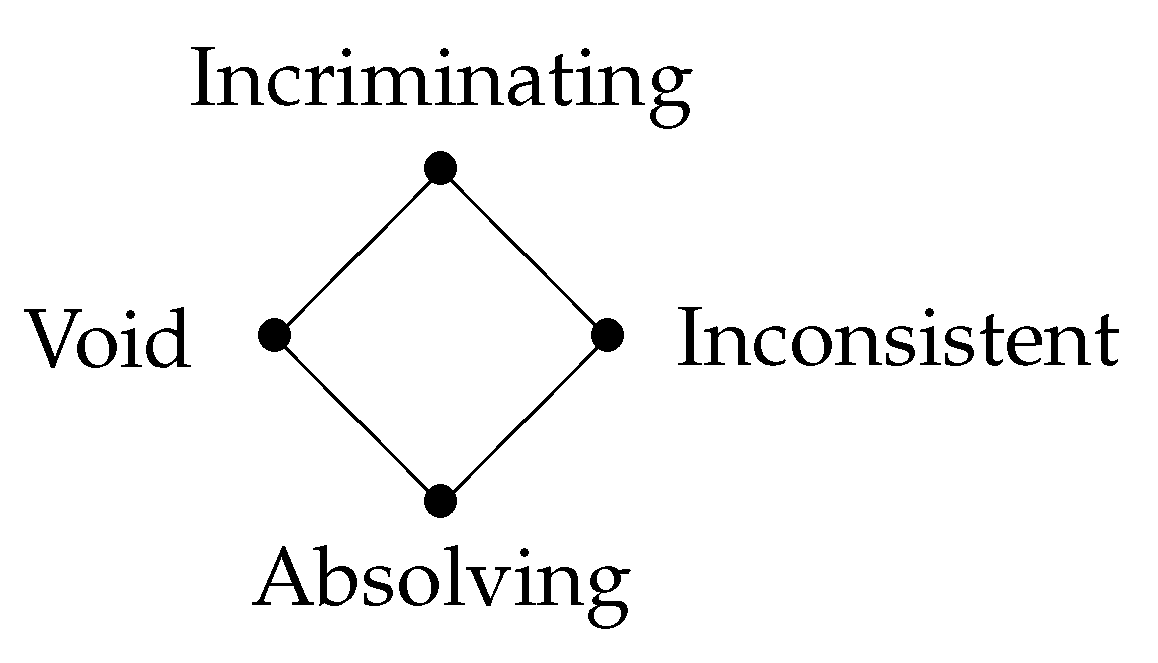
Example 1.

We are interested in applying the philosophy of Belnap’s four-valued logic [44] into forensics analysis. To this aim, any evidence in a forensics procedure will be associated with a truth-value in such logic, depending on what the evidence implies regarding the culpability of a certain suspect. In Belnap’s four-valued logic, the truth-values are: True, False, None (neither True nor False) and Both (both True and False). In our approach, these values are, respectively, interpreted as follows: Incriminating, Absolving, Void and Inconsistent. The resulting four-valued lattice is illustrated in Figure 2. Note that, Incriminating is a join-decomposable element, Absolving behaves like the bottom element and Void and Inconsistent are join-irreducible elements of $(L,⪯)$.

The meaning of Incriminating and Absolving is clear. In what concerns the truth-value Void, it may be caused for two reasons: either there is no evidence or there is a false evidence, that is, the information has been created or obtained illegally. Finally, evidence is considered to be Inconsistent if there are indications that the suspect is guilty and there are also indications that the suspect is innocent. For instance, this may happen if the evidence is collected twice, resulting in different outcomes. Undoubtedly, the nature of Void and Inconsistent is different, and therefore we must define them as different truth-values. Nevertheless, both values represent lack of verdict, and thus they are incomparable from the point of view of incrimination.

Now, assume that there are three kind of evidences in a certain criminal investigation: witness, video and DNA. The three of them can be related to a pair of values in $(L,⪯)$, one representing the content of the corresponding evidence, and the other one concerning the reliability of the evidence. Concretely, the witness is associated with the pair $(a_1,x_1)$ and video is related to $(a_2,x_2)$, where $a_1$/$a_2$ contains the grade of incrimination which the testimony/video record suggests, whilst $x_1$/$x_2$ indicates its reliability (the witness/video might be corrupted by noise, location, etc.). Similarly, DNA is related to the pair $(a_3,x_3)$, where $a_3$ represents the DNA matching and $x_3$ the level of reliability of the evidence. For instance, $x_3$ will be greater (more compromising) if there are plenty of DNA traces and they are found in key locations of the crime scene. Evidence is assumed to incriminate a suspect if both $a_j$ and $x_j$ incriminate the suspect. In other words, the level of incrimination of an evidence may be computed as the infimum of $a_j$ and $x_j$. Notice that the infimum operator of the lattice $(L,⪯)$ represented in Figure 2 coincides with the conjunction in Belnap’s logic. Besides, one piece of incriminating evidence is enough to blame the suspect. As a result, we may join the suggested incrimination of the evidences by taking the supremum.

The values $a_1,a_2,a_3$ can be collected in a first stage of a criminal investigation. However, deepening of the reliability of the evidences entails more efforts and time. As a consequence, it would be advantageous having a method to decide, from $a_1$, $a_2$ and $a_3$, if a certain suspect is a potential culprit of the crime, or if the evidence is not strong enough to question his innocence. Sup-equations can be used for this purpose. For instance, consider the sup-equation

$$(a_1 \& x_1)\vee (a_2 \& x_2)\vee (a_3 \& x_3)=\mathrm{Absolving}$$

(20)

where $\&$ represents the infimum operator. The solution set of (20) represents the number of possibilities to the suspect being innocent. Similarly, the solution set of the sup-equation

$$(a_1 \& x_1)\vee (a_2 \& x_2)\vee (a_3 \& x_3)=\mathrm{Incriminating}$$

(21)

would inform us about the feasibility of the suspect being the culprit of the crime.

According to the solution set of the preceding Equations (20) and (21), the forensics team could agree to collect more evidence, evaluate the reliability of the evidences or maybe investigate other suspects.

In the foregoing example, & is the unique conjunction appearing in (20) and (21), and the infimum operator & is a t-norm in the sense of [38]; that is, it is a commutative and associative operator. Hence, the theory developed in [38] is strong enough to solve (20) and (21), as well as similar equations with Void or Inconsistent in the right-hand side. Nevertheless, some situations require to work with a non-commutative and/or non-associative operator. Furthermore, in certain problems, different variables demand to use different conjunctions. In that case, the arising equations are not within the scope of the results in [38]. In what follows, as an extension of Example 1, we provide a forensics science context which gives rise to multi-adjoint sup-equations, and we employ the theory developed in this manuscript to solve such equations.

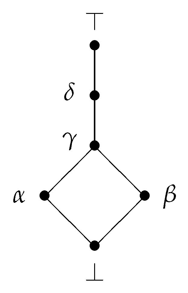
Example 2.

Consider the forensics context presented in Example 1. From a practical point of view, it would be desirable to have different grades of incrimination. Consequently, hereinafter we granulate the truth-value Incriminating according to the fortitude of the evidence, differentiating among Doubting innocence, Indicating involvement and Inculpating.

In order to model the new set of truth-values, we will make use of the complete lattice $(L,⪯)$, whose Hasse diagram is portrayed in Figure 3. Namely, the elements $\perp ,\alpha ,\beta ,\gamma ,\delta ,\top \in L$ represent the truth-values Absolving, Void, Inconsistent, Doubting innocence, Indicating involvement and Inculpating, respectively. Notice that, the lattice $(L,⪯)$ contains the bottom element ⊥; the join-irreducible elements $\alpha ,\beta ,\delta ,\top$; the join-decomposable element γ, which can be written as $\gamma =\alpha \vee \beta$.

Concerning the evidence—witness, video and DNA—we may have that witness and video deserve a treatment separate from DNA. For instance, the coincidence and the reliability of DNA are objective features. Nevertheless, if both the content and the reliability of a testimony or a video record are corrupted, then it is considered extenuating evidence in favour of the suspect. In other words, if the truth value of $a_1$ and $x_1$ is equal to α, then the conjunction of $a_1$ and $x_1$ is equal to ⊥, and similarly for $a_2$ and $x_2$. Since this does not hold for DNA, we require, then, two different conjunctions: A conjunction ${\&}_1$ to work with witness and video evidence and a generalization of Belnap’s conjunction ${\&}_2$ to work with the DNA evidence, satisfying $\alpha {\&}_1 \alpha =\perp$ and $\alpha {\&}_2 \alpha =\alpha$. This fact was not taken into account in Example 1 in order to set a preliminary forensics contextualization.

Other than that, if the testimony or a video record of a trusted source is corrupted—i.e., $a_1=\alpha$ and $x_1=\delta$ or $a_2=\alpha$ and $x_2=\delta$, the evidence is also considered to extenuate the suspect from the crime, that is, $\alpha {\&}_1 \delta =\perp$. This does not apply if the reliability of incriminating content is corrupted—i.e., $a_1=\delta$ and $x_1=\alpha$ or $a_2=\delta$ and $x_2=\alpha$. Thus, $\delta {\&}_1 \alpha =\alpha$, from which ${\&}_1$ is a non-commutative operator.

In what follows, we will make use of multi-adjoint sup-equations to answer the following questions:

(A) 

How possible it is a video record indicates that an innocent is involved in a crime?

(B) 

Provided a lightly inculpating testimony, an inconsistent video record and highly coincident DNA traces, what are the chances to the suspect being innocent? What about the possibilities to doubt about the innocence of the suspect?

Regarding the first query, we assume lack of witnesses and DNA traces. Hence, $a_1=a_3=\alpha$ and $a_2=\delta$ by hypothesis. Observe that the possibilities of the suspect being innocent are equivalent to the solution set of the multi-adjoint sup-equation

$$(\alpha {\&}_1 x)\vee (\gamma {\&}_1 y)\vee (\alpha {\&}_2 z)=\perp$$

(22)

Hereinafter, we will apply the results developed throughout this manuscript to solve (22), where the mappings ${\&}_1,{\&}_2:L\times L\to L$ are defined by Table 1. Note that, since the table corresponding to ${\&}_2$ is symmetric, the operator ${\&}_2$ is commutative. In what regards ${\&}_1$, as aforementioned, it is non-commutative since $\alpha {\&}_1 \delta =\perp$ whilst $\delta {\&}_1 \alpha =\alpha$. It is easy to check that the tuples $({\&}_1,{\swarrow }^1,{\nwarrow }_1)$ and $({\&}_2,{\swarrow }^2,{\nwarrow }_2)$ form adjoint triples, where the definition of ${\swarrow }^1,{\nwarrow }_1$ is detailed in Table 2 and the mappings ${\swarrow }^2,{\nwarrow }_2$ are given in Table 3. Obviously, as ${\&}_2$ is commutative, its residuated implications ${\swarrow }^2,{\nwarrow }_2$ coincide. Additionally, making the corresponding computations, the mappings ${⤣}_1$, , ${⤣}_2$, can be obtained, whose definitions are specified in Table 4.

Clearly, the lattices $M_3$ and $N_5$ are not sublattices of $(L,⪯)$ and thus, applying Theorem 1, $(L,⪯)$ is a distributive lattice. This leads us to assert that the tuple $(L,⪯,{\&}_1,{\swarrow }^1,{\nwarrow }_1,{\&}_2,{\swarrow }^2,{\nwarrow }_2)$ is a distributive biresiduated multi-adjoint lattice. Furthermore, we can check that the operators ${\&}_1,{\&}_2$ preserve the join and the meet, that is, they are homomorphisms. Hence, in short, the considered algebraic structure satisfies the hypothesis of the results developed in this manuscript.

According to Theorem 2, we obtain that the solution set of (22) is the interval $[\mathbf{\perp },(\perp {\nwarrow }_1\alpha ,\perp {\nwarrow }_1\gamma ,\perp {\nwarrow }_2\alpha )]$, that is, making the corresponding computations, the interval $\left[\right(\perp ,\perp ,\perp ),(\delta ,\alpha ,\beta \left)\right]$. Indeed, paying attention to Table 1, we can see that $\alpha {\&}_1 x=\perp$, for each $x\in \{\perp ,\alpha ,\beta ,\gamma ,\delta \}$; $\gamma {\&}_1 y=\perp$, for each $y\in \{\perp ,\alpha \}$, and $\alpha {\&}_2 z=\perp$, for each $z\in \{\perp ,\beta \}$.

Consequently, answering (A), we can assert that there are substantial possibilities for having a video record indicating that an innocent is involved in a crime. In what regards query (B), we will analyse the resolution of the sup-equation:

$$(\gamma {\&}_1 x)\vee (\beta {\&}_2 y)\vee (\delta {\&}_1 z)=\alpha$$

(23)

Notice that, in this case, (23) is a multi-adjoint sup-equation with join-irreducible right-hand side. In order to apply Theorem 4 to (23), let us check whether $s^1$, $s^2$ or $s^3$ belong to the set $S=\{s^h\mid \alpha ⪯a_h,\alpha {⤣}_{\sigma \left(h\right)}{a}_h⪯\alpha {\nwarrow }_{\sigma \left(h\right)}{a}_h\}$. Obviously, as , then $s^2\notin S$. In what regards $s^1$ and $s^3$, we have that $\alpha ⪯\gamma$ and $\alpha ⪯\delta$, respectively. On the one hand:

Therefore, we deduce that $s^1\notin S$. On the other hand, the following chain holds:

$$\begin{array}{ccc}\hfill \alpha {⤣}_1\delta & =\alpha ⪯\alpha =& \alpha {\nwarrow }_1\delta \hfill \end{array}$$

As a consequence, we conclude that $S=\left\{s^1\right\}=\left\{(\perp ,\perp ,\alpha {⤣}_1\delta )\right\}=\left\{(\perp ,\perp ,\alpha )\right\}$. Taking into account the aforementioned Theorem 4, the solution set of (23) is then the interval

$$[(\perp ,\perp ,\alpha ),(\alpha {\nwarrow }_1\gamma ,\alpha {\nwarrow }_2\beta ,\alpha {\nwarrow }_1\delta )]=[(\perp ,\perp ,\alpha ),(\alpha ,\alpha ,\alpha )]$$

In other words, the solutions of (23) are the tuples $(\perp ,\perp ,\alpha )$, $(\alpha ,\perp ,\alpha )$, $(\perp ,\alpha ,\alpha )$ and $(\alpha ,\alpha ,\alpha )$.

Coming back to query (B), we have found only four possibilities leading to no knowledge about the participation of the suspect in the crime. Thus, in most occasions, a lightly inculpating testimony, an inconsistent video record and highly coincident DNA traces will lead to some kind of verdict, either blaming or absolving, or some inconsistency.

From a theoretical point of view, the key role needs to be stressed, which plays the non-commutativity of ${\&}_1$ in the solvability of (23). In fact, if we consider its dual equation, it turns out to be unsolvable. Namely, let the multi-adjoint sup-equation

$$(x {\&}_1 \gamma )\vee (y {\&}_2 \beta )\vee (z {\&}_1 \delta )=\alpha$$

(24)

In this case, we have that

As a result, the corresponding set S of (24) is empty, and thus by Theorem 5 the solution set of (24) is also empty. Finally, in order to see the chances to blame the suspect at some grade of culpability, consider the multi-adjoint sup-equation given next:

$$(\gamma {\&}_1 x)\vee (\beta {\&}_2 y)\vee (\delta {\&}_1 z)=\gamma$$

(25)

Note that the coefficients of (25) coincide with the coefficients of (23). Nevertheless, the right-hand side of (25) has a different nature from the right-hand side of (23), since γ is a join-decomposable element of $(L,⪯)$. In particular, the set $\{\alpha ,\beta \}$ is a join-decomposition of γ—i.e., $\gamma =\alpha \vee \beta$.

In what follows, we will apply Theorem 6 to compute the solution set of (25). Following the notation of the mentioned theorem, we will use $S^1$ to denote the corresponding set of α and $S^2$ to denote the corresponding set of β. In other words, $S^1=\{s^{h1}\mid \alpha ⪯a_h,\alpha {⤣}_{\sigma \left(h\right)}{a}_h⪯\gamma {\nwarrow }_{\sigma \left(h\right)}{a}_h\}$ and $S^2=\{s^{h2}\mid \beta ⪯a_h,\beta {⤣}_{\sigma \left(h\right)}{a}_h⪯\gamma {\nwarrow }_{\sigma \left(h\right)}{a}_h\}$. Regarding $S^1$, we straightforwardly obtain that $s^{21}\notin S^1$, because . On the contrary, both $s^{11}$ and $s^{31}$ belong to $S^1$, since $\alpha ⪯\gamma$, $\alpha ⪯\delta$ and the following expressions hold:

$$\begin{array}{ccc}\hfill \alpha {⤣}_1\gamma & =\delta ⪯\top =& \gamma {\nwarrow }_1\gamma \hfill \\ \hfill \alpha {⤣}_1\delta & =\alpha ⪯\delta =& \gamma {\nwarrow }_1\delta \hfill \end{array}$$

As far as $S^2$ is concerned, we have that $\beta ⪯\gamma$, $\beta ⪯\beta$ and $\beta ⪯\delta$. Furthermore, the next inequalities are verified:

$$\begin{array}{ccc}\hfill \beta {⤣}_1\gamma & =\beta ⪯\top =& \gamma {\nwarrow }_1\gamma \hfill \\ \hfill \beta {⤣}_2\beta & =\beta ⪯\top =& \gamma {\nwarrow }_2\beta \hfill \\ \hfill \beta {⤣}_1\delta & =\beta ⪯\delta =& \gamma {\nwarrow }_1\delta \hfill \end{array}$$

Hence, we can assert that

$$\begin{array}{ccc}\hfill S^1& =& \{s^{11},s^{31}\}=\{(\alpha {⤣}_1\gamma ,\perp ,\perp ),(\perp ,\perp ,\alpha {⤣}_1\delta )\}=\{(\delta ,\perp ,\perp ),(\perp ,\perp ,\alpha )\}\hfill \\ \hfill S^2& =& \{s^{12},s^{22},s^{32}\}=\{(\beta {⤣}_1\gamma ,\perp ,\perp ),(\perp ,\beta {⤣}_2\beta ,\perp ),(\perp ,\perp ,\beta {⤣}_1\delta )\}=\{(\beta ,\perp ,\perp ),(\perp ,\beta ,\perp ),(\perp ,\perp ,\beta )\}\hfill \end{array}$$

Similarly, the tuple g related to (25) is defined as $g=(\gamma {\nwarrow }_1\gamma ,\gamma {\nwarrow }_2\beta ,\gamma {\nwarrow }_1\delta )=(\top ,\top ,\delta )$. We are now in a position to apply Theorem 6, from which the solution set of (25) can be written as

$$\bigcup _{\begin{array}{c}s\in S^1\\ t\in S^2\end{array}}\left[s\vee t,g\right]$$

Making the corresponding computations, we conclude that the solution set of (25) equals

$$\left[\right(\delta ,\perp ,\perp ),(\top ,\top ,\delta \left)\right]\cup \left[\right(\perp ,\perp ,\gamma ),(\top ,\top ,\delta \left)\right]\cup \left[\right(\beta ,\perp ,\alpha ),(\top ,\top ,\delta \left)\right]\cup \left[\right(\perp ,\beta ,\alpha ),(\top ,\top ,\delta \left)\right]$$

We conclude then that there is a great number of options to blame a suspect from a lightly inculpating testimony, an inconsistent video record and highly coincident DNA traces.

Notice that the minimal solutions $(\beta ,\perp ,\alpha )$ and $(\perp ,\beta ,\alpha )$ cannot be obtained from the results presented in [34], since those results only characterize minimal solutions with a single non-bottom component.

4. Conclusions

This paper has extended the results and properties introduced in [34,38] to the multi-adjoint framework. To the best of our knowledge, these papers considered the most general frameworks in which the analytical expression of the minimal solutions of FRE was given. The use of different conjunctions of a given distributive biresiduated multi-adjoint lattice has been allowed in the resolution of sup-equations and sup-inequalities. This fact notably extends the contribution presented in [38], since a more flexible framework can be considered where neither commutativity nor associativity are required on the conjunctions. In [34] the multi-adjoint character was not considered either. It is also important to mention that the results obtained for the minimal solutions of multi-adjoint sup-inequalities and multi-adjoint sup-equations improve the ones given in [34]. For instance, giving a complete characterization of all minimal solutions of the sup-equations.

Specifically, in this paper, the whole set of solutions of multi-adjoint sup-inequalities and multi-adjoint sup-equations has been analytically determined using a “dual” notion of residuated implication. Moreover, the solvability is based on the character of the independent term as the bottom, join-irreducible or join-decomposable element. Therefore, the whole set of solutions of all sup-equations and sup-inequalities on distributive biresiduated multi-adjoint lattices satisfying the descendent chain condition, has been analytically characterized. Thus, the results in this paper provide a general framework to model real applications, such as forensic analysis, medical diagnosis, decision support, among others, with a great level of flexibility and solve the obtained equations, computing all solutions immediately.

In the future, systems of multi-adjoint sup-equations and systems of multi-adjoint sup-inequalities will be studied, giving rise then to the resolution of multi-adjoint relation equations. Furthermore, the comparison with the methodologies based on concept lattices and the covering problem will be studied. Finally, we are interested in the consideration of negations in the sup-equations and sup-inequalities, with the aim of enhancing the knowledge on bipolar fuzzy relation equations [4,22,23].