Abstract
The Scher–Montroll model successfully describes subdiffusive photocurrents in homogeneously disordered semiconductors. The present paper generalizes this model to the case of fractal spatial disorder (self-similar random distribution of localized states) under the conditions of the time-of-flight experiment. Within the fractal model, we calculate charge carrier densities and transient current for different cases, solving the corresponding fractional-order equations of dispersive transport. Photocurrent response after injection of non-equilibrium carriers by the short laser pulse is expressed via fractional stable distributions. For the simplest case of one-sided instantaneous jumps (tunneling) between neighboring localized states, the dispersive transport equation contains fractional Riemann–Liouville derivatives on time and longitudinal coordinate. We discuss the role of back-scattering, spatial correlations induced by quenching of disorder, and spatiotemporal non-locality produced by the fractal trap distribution and the finite velocity of motion between localized states. We derive expressions for the photocurrent and transit time that allow us to determine the fractal dimension of the distribution of traps and the dispersion parameter from the time-of-flight measurements.
1. Introduction
In 1975, Scher and Montroll [] successfully interpreted the experimental data of the time-of-flight (TOF) experiment in amorphous semiconductors and, within the framework of a statistical model, explained the main laws governing the dispersive transport of charge carriers. The TOF technique is still a popular and important method to study charge drift and diffusion in low-conductivity semiconductors. In particular, it is utilized to study the features of charge transfer in perovskite solar cells [] and organic bulk heterojunctions []. In the usual TOF method, the photocurrent response is registered after the injection of non-equilibrium charge carriers by a short laser pulse near one of the electrodes. Between electrodes, a strong electric field (> V/cm) close to breakdown conditions is applied to the sample to eliminate the space charge effects and reduce the contribution of diffusion to the observed response. However, as we know from the Scher–Montroll model, strong dispersion can occur even for the case of one-sided motion due to the localization of charge carriers. The correct interpretation of the TOF measurements in inhomogeneous structures is still relevant and important. Various factors and characteristics affect the photocurrent relaxation. Among these factors are the density of states, inhomogeneities in the spatial distributions of localized states and the electric field, the morphology of the percolation region, recombination, etc. [,,,].
In various disordered semiconductors (amorphous, porous, heavily doped, etc.), a specific transient current signal is often observed, and it consists of two sections with power-law behavior,
The exponent called the dispersion parameter depends on the medium characteristics and may depend on temperature, and less often on field intensity. By analogy with normal transients, the parameter is called the transit time or time-of-flight, although it has a slightly different physical meaning. The experimentally established fact is that for dispersive transport:
where U is an applied voltage.
In studies [,], it was observed that the transient current curves in the – scale have the same form for different values of applied voltage and sample width. This property is inherent in many materials, and it was called the universality of transient current curves (see the details in []). The observation of these features for various disordered materials confirms the universality of transport properties and indicates the prevailing role of statistical laws. The statistical model proposed by Scher and Montroll [] successfully describes subdiffusive photocurrents in homogeneously disordered semiconductors. Carrier transfer in the Scher–Montroll model is a jump-like random walk process (so-called continuous time random walk (CTRW)) on the lattice, and charge carriers change their positions abruptly at random times. The carrier jumps in the direction of the applied external voltage are independent of each other, and the waiting times between consecutive jumps are independent, identically distributed random variables . For the realization of the main features of dispersive transport, the waiting times have to be characterized by a heavy-tailed power-law distribution:
As mentioned above, the Scher–Montroll model is developed for the case of spatially homogeneous disorder. However, some experiments and numerical simulations indicate that the disorder in complex semiconducting systems can be of a fractal (self-similar) type [,,,,,]. In the present work, the Scher–Montroll model is generalized to the case of the dispersive transport of photo-injected carriers in semiconducting nanocomposites with a fractal distribution of localized states over the sample. The conditions of the time-of-flight experiment are assumed. Within the generalized Scher–Montroll model taking the power-law distribution of distances between traps into account, we calculate charge carrier densities and transient current for different cases, solving the corresponding fractional-order diffusion equation.
2. Anomalous Diffusion Equation for Fractal Hopping
We consider a modification of the stochastic model of dispersive transport taking into account ballistic transfer and hopping with power-law distributions of jump lengths. The calculations are carried out mainly for the time-of-flight experiment. However, the solutions and transport equations can be modified and applied to the interpretation of other experimental techniques, including the method of space charge limited current (SCLC) and charge extraction by linearly increasing voltage (CELIV). In addition, the results of this work can be used to generalize the models of charge injection, transfer, and recombination in organic solar cells, FETs, and OLEDs in the case of using CNT nanocomposites instead of organic semiconductors.
The scheme of the TOF experiment is shown in Figure 1. Using photoexcitation with a short laser pulse, a spatially narrow layer of electron-hole pairs is created near one of the electrodes. The generated electron-hole pairs dissociate at the nearest electrode. Depending on the applied voltage, carriers of a certain type (for example, electrons) leave the film through this electrode, and carriers of another type (holes) are forced to pass through the film to the counter electrode. Using the detected transient current, one can determine the average time-of-flight of charge carriers (transit time) to the opposite contact, where is drift mobility, L the sample thickness, and F the electric field. To observe the relevant TOF signal, the following conditions have to be satisfied []. The dielectric relaxation time is large, and the time constant is small, compared with the transit time ; the concentration of non-equilibrium charge carriers is small enough, and the charges do not interact, while the SCLC-regime does not take place.
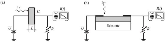
Figure 1.
The time-of-flight method in the vertical (a) and coplanar (b) structure.
The most important point of the Scher–Montroll theory is the power-law distribution of the localization times of charge carriers in physical models of hopping or multiple trapping. In more general CTRW models, applied not only to the dispersive transport problem, the jump lengths with a diverging second or first moment and correlations between jump lengths and waiting times are considered. We consider the application of generalized Scher–Montroll models to the description of dispersive transport and consider the possibility of identifying these modes using the TOF experiment.
The one-dimensional, decoupled version of the CTRW model [] assumes that the different jump lengths and waiting times between two consecutive jumps are independent random variables. For the description of anomalous diffusion, it is usually assumed that the distributions of the jump length and waiting time have the following (heavy-tailed) asymptotics:
If and , normal diffusion takes place in the diffusion limit (, ). All other values of and lead to anomalous diffusion with characteristic exponents . The Scher–Montroll model [] for dispersive transport in amorphous semiconductors corresponds to the case and . There was no evidence of the fractal distribution of localized states over a sample. Later experiments and numerical simulations indicated that the disorder in complex semiconducting systems can be of the fractal (self-similar) type [,,,,,]. In this work, we do not reject the case for dispersive transport of charge carriers and compute the corresponding TOF characteristics for the cases of instantaneous hops and for asymmetric Lévy walks with finite velocity.
For the given distributions of jump lengths and waiting times, the main asymptotic term of the probability density function satisfies the fractional diffusion equation (see, e.g., [,]):
Here:
is the Riemann–Liouville fractional derivative of order and is a fractional operator that can be defined via its Fourier transform or expressed via the Feller operator (see details in []). Here, is an asymmetry parameter. For the symmetric case, is a one-dimensional fractional Laplacian.
The solution of this fractional partial differential equation has a self-similar form and can be expressed via fractional stable densities [,]:
where:
is expressed through the Lévy stable densities, and . The latter densities can be determined by their characteristic functions [],
Here, is the asymmetry parameter, where . The width of the anomalous diffusion packet is . If , we have a subdiffusive regime, and when , superdiffusion is observed.
An important case for this study is the one-sided random walk, characterized by the probability density:
The papers [,,] considered a random walk of a particle along a one-dimensional stochastic fractal (so-called Lévy–Lorentz gas). This Lévy–Lorentz gas is a set of points located on an axis along which the particle walks. Each fractal implementation is constructed in such a way that random distances between different pairs of neighbors are independent and identically distributed according to the heavy-tailed power distribution with the exponent . A particle performs instantaneous jumps between neighboring sites that delay and hold it for a random period of T. Successive periods are independent, identically distributed random variables characterized by a power-type distribution with exponent . In [], an asymptotic solution of the diffusion problem on such a fractal was found for the general case of an asymmetric walk. The basic equations for diffusion on fractals were obtained. The results were compared with fractal walks, when the lengths of successive jumps are independent of their directions. Due to correlations of successive jumps of a walker, in the general case, the fundamental solutions of diffusion on a fractal and fractal diffusion differ significantly from each other, but both solutions are expressed in terms of stable Lévy densities and satisfy diffusion equations with fractional derivatives [].
3. Transient Current for One-Sided Fractal Hopping
The TOF method implies measuring the photocurrent response after injection of nonequilibrium carriers by a short laser pulse. As a rule, a strong electric field (> V/cm) is applied to the sample, close to the breakdown conditions of the dielectric, in order to avoid the effects of space charge and bipolar carrier transport and to reduce the contribution of diffusion. For the one-sided case, when and , the correlations between jump lengths in the model of a random walk on the Lévy–Lorentz fractal gas disappear, and the solutions in both models coincide [,].
The photocurrent can be calculated by integrating the electric current density,
It can be expressed in terms of the concentration of injected nonequilibrium carriers according to the following formula:
which can be obtained from the previous one with the continuity equation:
where N is the number of photoinjected carriers and is the probability density function of the charge carrier coordinate.
For a given carrier concentration:
the electric current density is:
Therefore, for the transient current (6), we obtain:
There are several special cases for specific parameter values. The transient current for the one-sided Lévy flight has the form:
If , we have:
In the case of subdiffusive transport () in a homogeneous 1D system,
For a special case of dispersive transport () in a fractal sample (),
For normal drift, a current step is observed:
where is the Heaviside step function.
For asymptotic estimates of Formula (8), it is necessary to know the asymptotic behavior of the fractional stable density. It is known that for the one-sided fractional stable density [],
Using the latter expression and Formula (8), we derive the expression for the asymptotic behavior of the transient current:
Thus, the transient current curves on a double logarithmic scale consist of two linear sections and the region corresponding to the transition mode. These curves have a universal shape, as in the case of the usual dispersive transport [].
The transit time corresponds to a kink in the log-log plot of the transient current and can be found by crossing the asymptotic behavior of the photocurrent (13) at small and large times,
The latter formula shows that at a constant temperature and field strength, the transit time scaling is .
The transient current curves calculated using Formulas (9)–(12) are presented in Figure 2. There are four important cases, normal drift , dispersive drift , one-sided Lévy flight with trapping , and the Lévy flight with the exponential distribution of waiting times . The slopes of in the log-log scale are determined by the dispersion parameter and are independent of . For the Lévy flight with trapping, we observe a longer smoothed transition period between two asymptotic decays. Thus, dispersion parameter can be determined from the slopes of in the log-log scale, and fractal parameter can be extracted from the scale dependence of the transit time on sample width L ().
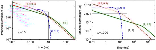
Figure 2.
Transient current curves for different pairs (; ). (Left) ; (right) .
4. Transient Current for the Lévy Walk
In the previous section, we obtained an expression for the transient current within the fractal walk model with instantaneous hops. In this section, we will consider motion with a finite constant velocity (Lévy walk). The integral equation for the one-sided random walk with trapping and free motion with constant velocity has the form:
where the densities of transitions from the localized state to the state of motion and vice versa are related by the following relations:
Here, we assume the initial condition . The particle starts from a localized state with probability and from a delocalized state with probability .
Usually, the Fourier transform in the coordinate and the Laplace transform in time are applied in order to pass from integral equations to algebraic ones. In our case, the functions are defined on , and we apply the double Laplace transformation with respect to x and time t.
From Equation (14), we obtain:
For the transforms of transitions densities, we have the following system:
Solving the latter system, we arrive at expressions for and ,
Substituting the latter formulae into (15), we get the following transform:
Under the assumption that all charge carriers started the process from a localized state , , the expression is simplified:
Under the assumption of power-law distributions of waiting times in traps and the power-law distribution of path lengths,
After substituting the latter expressions in the transform of the asymptotic solution (17), we obtain:
Introducing and rewriting the latter expression in the form:
Inverting it, we arrive at the following equation:
containing the fractional Riemann–Liouville derivative of order with respect to time and the material derivative of fractional order . We find the solution by inverting the transform:
using the known expressions for fractional stable densities []. Given that:
we find:
The rule for permuting the indices of a one-sided fractional stable distribution has the form []:
For densities, it can be written as:
As a result, we arrive at the following asymptotic solution for one-sided Levy walks:
Figure 3 demonstrates the comparison of these pdfs for different values of and K with the results of the Monte Carlo simulation. Thus, we made sure that Formula (18) perfectly describes the asymptotic distribution densities of charges for a one-sided Lévy walk with trapping. For the simulation of waiting times and path lengths, we use densities in the form of “fractional exponentials” (see, e.g., []),
for which expressions for the Monte Carlo simulation are known []:
Here, and are one-sided stable random variables of order and .
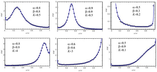
Figure 3.
Charge carrier distribution (pdf) for different values of and K in comparison with the Monte Carlo simulation results.
If , the fractional stable density is expressed in terms of elementary functions:
and the solution represents the Lamperti function:
In the particular case of , the solution takes the form:
Substituting these solutions into expression:
we compute the transient current density for different situations.
The calculated transient current curves compared with the Monte Carlo simulation are presented in Figure 4. The excellent agreement is a consequence of valid solutions (18). The family of transient current curves for various values of and K is demonstrated in Figure 5.
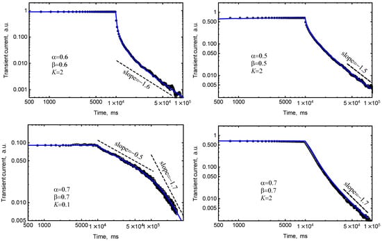
Figure 4.
Transient current curves for various values of and K in comparison with the Monte Carlo simulation results.
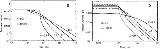
Figure 5.
Theoretical transient current curves for various values of (a) and K (b). Other parameters are indicated in figure.
In the asymptotics of , the solution (18) goes into the following:
If , the expression (19) is valid for the entire concentration of nonequilibrium carriers inside the sample. Up to the normalization constant, the solution (19) coincides with the solution (7) for instantaneous hopping. The time point corresponds to the passage time of the sample boundary by a ballistic front. A kink in the transient current curves corresponding to the transit time obtained in Section 3 should also be observed in the case of Lévy walks. In other words, on the transient current curves for Lévy walks, two kinks can be observed corresponding to the time the front reaches the boundary and the time the “center of gravity” of charge carriers crosses the boundary . The presence of these two kinks is well observed for the case (see Figure 6).

Figure 6.
Transient current curves for different values of and K.
It is important to note that the obtained transient current curves combine the features characteristic of normal transport (the presence of a plateau and ballistic transit time) and the dispersive power-law tail.
Simulations show that back-scattering results in smearing of the transient current curves and to the smoother kinks indicated above. Moreover, back-scattering leads to the increased role of correlations between consecutive jump lengths in the case of fixed localized states []. However, these nuances require additional research.
5. Conclusions
The Scher–Montroll model of dispersive transport in samples with spatially homogeneous disorder is successfully applied to describe the transient photocurrent in semiconductors with an amorphous structure, including organic ones. In this work, the Scher–Montroll model is generalized to the case of the dispersive transport of photo-injected carriers in nanocomposites with a fractal distribution of localized states. The influence of ballistic transport is taken into account in the framework of the hopping model with heavy-tailed distributions of jumps. The calculations are carried out within the framework of the time-of-flight method. Criteria are established that make it possible to determine the fractal dimension of the distribution of traps from the transition current curves. The dispersion parameter can be determined from the slopes of on a double logarithmic scale, as in the standard model of dispersive transport, and the fractal distribution parameter can be extracted from the power-law dependence of the transit time on the sample width L. For the case of the Lévy walk with a finite velocity, transient current curves with a plateau and a slowly decaying power-law tail are predicted. In nanocomposites, the plateau can arises due to ballistic transport along nanotubes, or the molecular chains of a conjugated polymer, and power-law relaxation due to the localization of charge carriers. For Lévy walks, two kinks in the transient current curves can be observed corresponding to the time the front reaches the boundary and the time the “center of gravity” of charge carriers crosses the boundary . The presence of these two kinks is well identified for the case . The obtained transient current curves combine the features characteristic of normal transport (the presence of a plateau and ballistic transit time) and the dispersive power-law tail.
Funding
This research was funded by the Russian Science Foundation (grant 19-71-10063). The author acknowledges financial support from the Ministry of Science and Higher Education of the Russian Federation (Project 0004-2019-0001).
Conflicts of Interest
The author declares no conflict of interest.
References
- Scher, H.; Montroll, E.W. Anomalous transit-time dispersion in amorphous solids. Phys. Rev. B 1975, 12, 2455. [Google Scholar] [CrossRef]
- Maynard, B.; Qi, L.; Schiff, E.A.; Yang, M.; Zhu, K.; Kottokkaran, R.; Abbas, H.; Dalal, V.L. Electron and hole drift mobility measurements on methylammonium lead iodide perovskite solar cells. Appl. Phys. Lett. 2016, 108, 173505. [Google Scholar] [CrossRef]
- Morfa, A.J.; Nardes, A.M.; Shaheen, S.E.; Kopidakis, N.; Van De Lagemaat, J. Time-of-Flight Studies of Electron-Collection Kinetics in Polymer: Fullerene Bulk-Heterojunction Solar Cells. Adv. Funct. Mater. 2011, 21, 2580–2586. [Google Scholar] [CrossRef]
- Bonch-Bruevich, V.; Enderlein, R.; Esser, B.; Keiper, R.; Mironov, A.; Zvyagin, I. Electron Theory of Disordered Semiconductors; VEB Deutscher Verlag der Wissenschaften: Berlin, Germany, 1984. [Google Scholar]
- Tiedje, T.; Rose, A. A physical interpretation of dispersive transport in disordered semiconductors. Solid State Commun. 1981, 37, 49–52. [Google Scholar] [CrossRef]
- Zvyagin, I. Kinetic Phenomena in Disordered Semiconductors; Moscow State University Press: Moscow, Russia, 1984. (In Russian) [Google Scholar]
- Bulyarskii, S.; Grushko, N. Generalized model of recombination in inhomogeneous semiconductor structures. J. Exp. Theor. Phys. 2000, 91, 1059–1065. [Google Scholar] [CrossRef]
- Pfister, G.; Scher, H. Dispersive (non-Gaussian) transient transport in disordered solids. Adv. Phys. 1978, 27, 747–798. [Google Scholar] [CrossRef]
- Pook, W.; Janßen, M. Multifractality and scaling in disordered mesoscopic systems. Z. Phys. B Condens. Matter 1991, 82, 295–298. [Google Scholar] [CrossRef]
- Hegger, H.; Huckestein, B.; Hecker, K.; Janssen, M.; Freimuth, A.; Reckziegel, G.; Tuzinski, R. Fractal conductance fluctuations in gold nanowires. Phys. Rev. Lett. 1996, 77, 3885. [Google Scholar] [CrossRef] [PubMed]
- Barthelemy, P.; Bertolotti, J.; Wiersma, D.S. A Lévy flight for light. Nature 2008, 453, 495. [Google Scholar] [CrossRef] [PubMed]
- Kohno, H.; Yoshida, H. Multiscaling in semiconductor nanowire growth. Phys. Rev. E 2004, 70, 062601. [Google Scholar] [CrossRef] [PubMed]
- Kohno, H. Self-organized nanowire formation of Si-based materials. In One-Dimensional Nanostructures; Springer: Berlin/Heidelberg, Germany, 2008; pp. 61–78. [Google Scholar]
- Raboutou, A.; Peyral, P.; Lebeau, C.; Rosenblatt, J.; Burin, J.P.; Fouad, Y. Fractal vortices in disordered superconductors. Phys. A Stat. Mech. Appl. 1994, 207, 271–279. [Google Scholar] [CrossRef]
- Köhler, A.; Bässler, H. Electronic Processes in Organic Semiconductors: An Introduction; John Wiley & Sons: Hoboken, NJ, USA, 2015. [Google Scholar]
- Montroll, E.W.; Weiss, G.H. Random walks on lattices. II. J. Math. Phys. 1965, 6, 167–181. [Google Scholar] [CrossRef]
- Saichev, A.I.; Zaslavsky, G.M. Fractional kinetic equations: Solutions and applications. Chaos Interdiscip. J. Nonlinear Sci. 1997, 7, 753–764. [Google Scholar] [CrossRef] [PubMed]
- Metzler, R.; Klafter, J. The random walk’s guide to anomalous diffusion: A fractional dynamics approach. Phys. Rep. 2000, 339, 1–77. [Google Scholar] [CrossRef]
- Uchaikin, V.V. Self-similar anomalous diffusion and Levy-stable laws. Physics-Uspekhi 2003, 46, 821. [Google Scholar] [CrossRef]
- Kolokoltsov, V.; Korolev, V.; Uchaikin, V. Fractional stable distributions. J. Math. Sci. 2001, 105, 2569–2576. [Google Scholar] [CrossRef]
- Uchaikin, V.V.; Zolotarev, V.M. Chance and Stability: Stable Distributions and their Applications; Walter de Gruyter: Berlin, Germany, 1999. [Google Scholar]
- Barkai, E.; Fleurov, V.; Klafter, J. One-dimensional stochastic Lévy-Lorentz gas. Phys. Rev. E 2000, 61, 1164. [Google Scholar] [CrossRef] [PubMed]
- Uchaikin, V. Anomalous diffusion on a one-dimensional fractal Lorentz gas with trapping atoms. In Emergent Nature: Patterns, Growth and Scaling in the Sciences; World Scientific: Singapore, 2001; pp. 411–421. [Google Scholar]
- Uchaikin, V.; Sibatov, R. Lévy Walks on a One-Dimensional Fractal Lorentz Gas with Trapping Atoms; Mathematics and Statistics Research Report Series; The Nottingham Trent University Preprints: Nottingham, UK, 2004. [Google Scholar]
- Uchaikin, V.V.; Cahoy, D.O.; Sibatov, R.T. Fractional processes: From Poisson to branching one. Int. J. Bifurc. Chaos 2008, 18, 2717–2725. [Google Scholar] [CrossRef]
Publisher’s Note: MDPI stays neutral with regard to jurisdictional claims in published maps and institutional affiliations. |
© 2020 by the author. Licensee MDPI, Basel, Switzerland. This article is an open access article distributed under the terms and conditions of the Creative Commons Attribution (CC BY) license (http://creativecommons.org/licenses/by/4.0/).