Article

A Meshless Method Based on the Laplace Transform for the 2D Multi-Term Time Fractional Partial Integro-Differential Equation

1
Department of Mathematics, Islamia College Peshawar, Peshawar 25000, Khyber Pakhtoon Khwa, Pakistan
2
Department of Mathematics, University of Lakki Marwat, Lakki Marwat 28420, Khyber Pakhtunkhwa, Pakistan
3
KMUTT Fixed Point Research Laboratory, Room SCL 802 Fixed Point Laboratory, Science Laboratory Building, Department of Mathematics, Faculty of Science, King Mongkut’s University of Technology Thonburi (KMUTT), 126 Pracha-Uthit Road, Bang Mod, Thung Khru, Bangkok 10140, Thailand
4
Department of Medical Research, China Medical University Hospital, China Medical University, Taichung 40402, Taiwan
5
College of Science Department of Mathematics, Northern Border University, Arar 73222, Saudi Arabia
*
Author to whom correspondence should be addressed.
Mathematics 2020, 8(11), 1972; https://doi.org/10.3390/math8111972
Submission received: 8 October 2020 / Revised: 1 November 2020 / Accepted: 3 November 2020 / Published: 6 November 2020
(This article belongs to the Special Issue Applications of Partial Differential Equations in Engineering)

Abstract

:
In this article, we propose a localized transform based meshless method for approximating the solution of the 2D multi-term partial integro-differential equation involving the time fractional derivative in Caputo’s sense with a weakly singular kernel. The purpose of coupling the localized meshless method with the Laplace transform is to avoid the time stepping procedure by eliminating the time variable. Then, we utilize the local meshless method for spatial discretization. The solution of the original problem is obtained as a contour integral in the complex plane. In the literature, numerous contours are available; in our work, we will use the recently introduced improved Talbot contour. We approximate the contour integral using the midpoint rule. The bounds of stability for the differentiation matrix of the scheme are derived, and the convergence is discussed. The accuracy, efficiency, and stability of the scheme are validated by numerical experiments.

1. Introduction

Recently, the theory fractional calculus has gained significant attention in the field of engineering and other sciences because of its various applications in modeling numerous phenomena. For example numerous phenomena in the mathematical biology, physics, and engineering fields can be described by fractional integro-differential equations (FIDEs), fractional partial integro-differential equations (FPIDEs), and fractional partial differential equations (FPDEs). In particular, several phenomena give rise to fractional partial integro-differential equations such as viscoelastic phenomena, signal processing, and fluid mechanics (see [1,2,3,4] and the references therein).
Finding exact or numerical solutions of FPIDEs with weakly singular kernels is an important task. Due to the possible singularities of the kernel function at the origin [5], sharp changes will occur in the solution, so the exact/analytic solution may be difficult to obtain [6]. Therefore, the alternate way is to develop an accurate numerical scheme. The approximation of FPIDEs and partial integro-differential equations (PIDEs) has been considered by many researchers, such as the authors in [7,8,9,10], who used the finite difference (FDM) and finite element (FEM) methods for the approximation of PIDEs. The authors in [11,12] used spline collocation methods for approximating PIDEs of the parabolic and hyperbolic type, respectively. Huang [13] solved parabolic PIDEs using the time discretization scheme. In [3], the B-spline solution of FPIDEs was found. The authors in [4] used the reproducing kernel method for the approximation of FPIDEs. A backward Euler difference scheme was constructed for the approximation of the partial integro-differential equation with multi-term kernels [14]. Other valuable work on integro-differential equations can be found in [15,16,17,18,19,20,21,22,23,24,25,26] and the references therein. Recently, the meshless methods have attracted researchers and become the primary tool for interpolating multidimensional scattered data.
In the literature, we can find a large number of meshless methods developed for the numerical treatment of different PDEs or PIDEs such as the authors in [27], who proposed the RBF-FD method for the approximation of PIDEs. In [28], a local method was developed for the approximation of PIDEs. In [29], the nonlinear PIDEs were approximated via the RBF and theta method. Similarly, the authors in [30] proposed a local method with the optimal shape parameter for PIDEs.
In this article, the Laplace transform and localized meshless method are combined for the approximation of the solution of FPIDEs with a weakly singular kernel. In the literature, we can find some valuable work on the Laplace transform coupled with other methods in [31,32,33,34,35,36,37,38,39] and the references therein. We consider an FPIDE of the form [40]:
ρ = 1 m d ρ D τ γ ρ U ( ζ , τ ) ( α ) L U ( ζ , τ ) = f ( ζ , τ ) , ζ Ω , and τ [ 0 , T ] ,
subject to the initial and boundary conditions:
U ( ζ , 0 ) = Θ ( ζ ) , ζ Ω , B U ( ζ , τ ) = h ( ζ , τ ) , ζ Ω , τ [ 0 , T ] .
where 0 < γ 1 γ 2 γ m 1 , d ρ > 0 , m N ,   Ω = [ 0 , L ] 2 , Θ is a given function,  L = Δ , and B is the boundary operators. D τ γ is the Caputo derivative of order γ defined as [41,42]:
D τ γ U ( τ ) = 1 Γ ( p γ ) 0 τ ( τ θ ) p γ 1 d p d θ p U ( θ ) d θ , p 1 γ p , p N ;
in particular for p = 1 , we have:
D τ γ U ( τ ) = 1 Γ ( 1 γ ) 0 τ ( τ θ ) γ d d θ U ( θ ) d θ , 0 γ 1 ,
and the α th integral ( α ) U ( τ ) is defined as [42]:
( α ) U ( τ ) = 1 Γ ( α ) 0 τ ( τ θ ) α 1 U ( θ ) d θ .
The Laplace transform of U ( τ ) is defined by:
U ^ ( s ) = L { U ( τ ) } = 0 e s τ U ( τ ) d τ ,
and the Laplace transform of D τ γ is given by:
L { D τ γ U ( τ ) } = s γ U ^ ( s ) i = 0 m 1 s γ i 1 U ( i ) ( 0 ) ,
while the Laplace transform of ( α ) U ( τ ) is given by:
L { ( α ) U ( τ ) } = 1 Γ ( α ) Γ ( α ) U ^ ( s ) s α .
Equation (1) involves multi-term time fractional derivatives, which are helpful in modeling complex physical systems such as the physical multi-rate phenomenon [43], fractional Zener model [44], heavily damped motion, Newtonian fluid [42,45], and anomalous relaxation process [46]. The integral term represents the viscosity part of Equation (1) [40]. Equation (1) can be obtained from the partial integro-differential equation:
U ( ζ , τ ) τ ( α ) L U ( ζ , τ ) = f ( ζ , τ ) , ζ Ω , τ [ 0 , T ] ,
by replacing the first order time derivative by a linear combination of fractional derivatives of different orders [47]. For m = 1 , Equation (1) becomes the single term FPIDE of the form:
d 1 D τ γ 1 U ( ζ , τ ) ( α ) L U ( ζ , τ ) = f ( ζ , τ ) , ζ Ω , τ [ 0 , T ] ,
and for α = 1 , Equation (1) becomes the fractional multi-term diffusion equation:
ρ = 1 m d ρ D τ γ ρ U ( ζ , τ ) L U ( ζ , τ ) = f ( ζ , τ ) , ζ Ω , τ [ 0 , T ] .

2. Proposed Numerical Scheme

Taking the Laplace transform of Equations (1) and (2), we have:
d 1 s γ 1 U ^ ( ζ , s ) d 1 s γ 1 1 Θ ( ζ ) + d 2 s γ 2 U ^ ( ζ , s ) d 2 s γ 2 1 Θ ( ζ ) + + d m s γ m U ^ ( ζ , s ) d m s γ m 1 Θ ( ζ ) s α L U ^ ( ζ , s ) = f ^ ( ζ , s ) ,
B { U ^ ( ζ , s ) } = h ^ ( ζ , s ) ;
combining the like terms, we obtain the following system:
( d 1 s γ 1 I + d 2 s γ 2 I + d m s γ m I s α L ) U ^ ( ζ , s ) = g ^ ( ζ , s ) ,
B { U ^ ( ζ , s ) } = h ^ ( ζ , s ) ,
where:
g ^ ( ζ , s ) = d 1 s γ 1 1 Θ ( ζ ) + d 2 s γ 2 1 Θ ( ζ ) + + d m s γ m 1 Θ ( ζ ) + f ^ ( ζ , s ) ,
where I is the identity operator and L and B are the governing and the boundary differential operators. In order to solve the system given in (11) and (12), first, we employ the local meshless method to discretize the operators L and B . When we are done with the discretization of these two operators, the system of Equations (11) and (12) is solved in parallel for each point s along some suitable path Γ in the complex plane (see, e.g., [16,34]). Finally, the solution of the original problem (1) and (2) is obtained using the inverse Laplace transform. The local meshless method for the discretization of the given differential operators L and B is described in the next section.

2.1. Localized Meshless Method

In the localized meshless method for a given set of nodes { ζ i } i = 1 N Ω , the local meshless approximate of the function U ^ ( ζ ) has the form [48]:
U ^ ( ζ i ) = ζ h Ω i λ h i ϕ ( ζ i ζ h ) ,
where ϕ ( r ) is a radial kernel, r = ζ i ζ h is the distance between ζ i and ζ h , λ i = { λ h i } h = 1 n is the vector of expansion coefficients, Ω is the global domain, and Ω i is a local domain containing ζ i , and n nodes around it. Hence, we obtain N linear systems of order n × n given by:
U ^ i = Φ i λ i , i = 1 , 2 , 3 , , N ;
the elements of the system matrix Φ i are b l j i = ϕ ( ζ l ζ h ) , where ζ l , ζ h Ω i , and the unknowns λ i = { λ h i } h = 1 n are found by solving each n × n system. Next, the operator L U ^ ( ζ ) is approximated by:
L U ^ ( ζ i ) = ζ h Ω i λ h i L ϕ ( ζ i ζ h ) .
The above Equation (15) can be expressed as:
L U ^ ( ζ i ) = λ i · ν i ,
where λ i is an n-column vector and ν i is an n-row vector with entries:
ν i = L ϕ ( ζ i ζ h ) , ζ h Ω i ;
solving Equation (14), for λ i , we have,
λ i = ( Φ i ) 1 U ^ i .
From Equation (18), we use λ i in Equation (16) and get,
L U ^ ( ζ i ) = ν i ( Φ i ) 1 U ^ i = w i U ^ i ,
where,
w i = ν i ( Φ i ) 1 .
Thus, the local meshless approximation for the differential operator L at each center ζ i is given as:
L U ^ D U ^ .
The differentiation matrix D is sparse and has order N × N containing n number of non-zero entries, where n Ω i . The matrix D approximates the linear differential operator L . The approximation for the boundary differential operator B can be done in the same way.

3. Numerical Inversion of the Laplace Transform

Following the discretization by the local meshless method of the linear differential and boundary operators L and B , respectively, the system (11) and (12) is solved in parallel for each point s along some suitably chosen path in the complex plane. Finally, we get the solution of the problem (1) and (2) using the inversion formula:
U ( ζ , τ ) = 1 2 π i σ i σ + i e s τ U ^ ( ζ , s ) d s = 1 2 π ι Γ e s τ U ^ ( ζ , s ) d s , σ > σ 0 ,
where σ 0 R is called the converging abscissa and Γ is an initially appropriately chosen line connecting σ i to σ + i . This means all the singularities of U ^ ( ζ , s ) lie in the half plane R e s < σ . The approximation of the integral (22) is hard because of the slow decaying transform U ^ ( ζ , s ) and the highly oscillatory exponential factor e s τ . To handle these issues, we use the strategy suggested by Talbot [49]. He suggested the deformation of the contour of integration Γ . In particular, he suggested that the contour Γ be deformed in such a way that its real part starts and ends in the left half plane, and it encloses all the singularities of the transform U ^ ( ζ , s ) . Cauchy’s theorem allows such a deformation provided that U ^ ( ζ , s ) has no singularities on the contour [49]. On such contours, the exponential factor decays rapidly, which makes the integral in Equation (22) suitable for approximation using the midpoint or trapezoidal rule [49,50,51]. We consider a Hankel contour with the parametric form given by [50]:
Γ : s = s ( ϑ ) , π ϑ π ,
where R e s ( ± π ) = , and s ( ϑ ) is defined as:
s ( ϑ ) = M τ θ ( ϑ ) , θ ( ϑ ) = σ + μ ϑ cot ( γ ϑ ) + ν ι ϑ ,
where the parameters σ , γ , μ , and ν are to be described by the user. From Equations (22) and (24), we have:
U ( ζ , τ ) = 1 2 π i Γ e s τ U ^ ( ζ , s ) d s = 1 2 π i π π e s ( ϑ ) τ U ^ ( ζ , s ( ϑ ) ) s ( ϑ ) d ϑ .
We use the M-panel midpoint rule with uniform spacing k = 2 π M to approximate the integral in Equation (25) as:
U k ( ζ , τ ) = 1 M i j = 1 M e s j τ U ^ ( ζ , s j ) s ´ j , for ϑ j = π + ( j 1 2 ) k , s j = s ( ϑ j ) , s j = s ( ϑ j ) .

4. Convergence and Accuracy

In order to approximate the solution of FPIDEs using our proposed numerical scheme, the Laplace transform and local meshless method are used. In our numerical scheme, we employ the Laplace transform to the time dependent equation, which eliminates the time variable, and this process causes no error. Then, the local meshless method is utilized for approximating the time independent equation. The error estimate for local meshless method is of order O ( η 1 ϵ h ) ; 0 < η < 1 ; ϵ is the shape parameter; and h is the fill distance [52]. In the process of approximating the integral in Equation (25), we achieve the convergence at different rates depending on the path Γ . While approximating the integral in Equation (25), the convergence order relies on the step k of the quadrature rule and the time domain [ t 0 , T ] for Γ . In order to achieve high accuracy, we need to search for the most favorable values of the parameters involved in Equation (24). The authors [50] obtained the most suitable values of the parameters given as:
σ = 0.6122 , μ = 0.5017 , ν = 0.2645 , and γ = 0.6407 ,
with the corresponding error estimate as:
Error Estimate = | U ( ζ , τ ) U k ( ζ , τ ) | = O ( e 1.358 M ) .
The optimal contour is supposed to pass neither too close to nor too far from the singularities, in which case e s τ becomes too large. Moreover, to achieve the desired accuracy, the quadrature points are required to extend far enough into the left half plane. However, their contributions must not be less than the required accuracy.
The necessary steps of our method are presented in the following Algorithm 1.
Algorithm 1.
1:
Input: The computational domain, the fractional order derivative in [0,1], the final time, the contour of integration, the initial shape parameter and the other parameter of the given model, the inhomogeneous function, and other conditions.
2:
Step 1: Apply the Laplace transform to the problem (1) and (2), and obtain the time independent problem (11) and (12).
3:
Step 2: Discretize the linear differential operator L and boundary operator B using (21).
4:
Step 3: Solve the system of Equations (11) and (12) in parallel for each point s along the contour of integration Γ given in (18).
5:
Step 4: Compute the approximate solution using (25).
6:
Output: The approximate solution is U k ( ζ , τ ) .

5. Stability Analysis

In order to investigate the system (11) and (12) stability, we represent the system in discrete form as:
Y U ^ = b ,
where Y N × N is the sparse differentiation matrix obtained using the local meshless method described in Section 2.1. For the system (27), the constant of stability is given by:
C = sup U ^ 0 U ^ Y U ^ ,
where the constant C is finite for any discrete norm . defined on R N . From (28), we may write:
Y 1 U ^ Y U ^ C ,
Similarly, for the pseudoinverse Y of Y, we can write:
Y = sup v 0 Y v v .
Thus, we have:
Y sup v = Y U ^ 0 Y Y U ^ Y U ^ = sup U ^ 0 U ^ Y U ^ = C .
We can see that Equations (29) and (31) confirm the bounds for the stability constant C. Calculating the pseudoinverse for approximating the system in Equation (27) numerically can be difficult computationally, but it ensures the stability. MATLAB’s function condest can be used to estimate Y 1 in the case of square systems; thus, we have:
C = c o n d e s t ( Y ) Y .

6. Numerical Results and Discussion
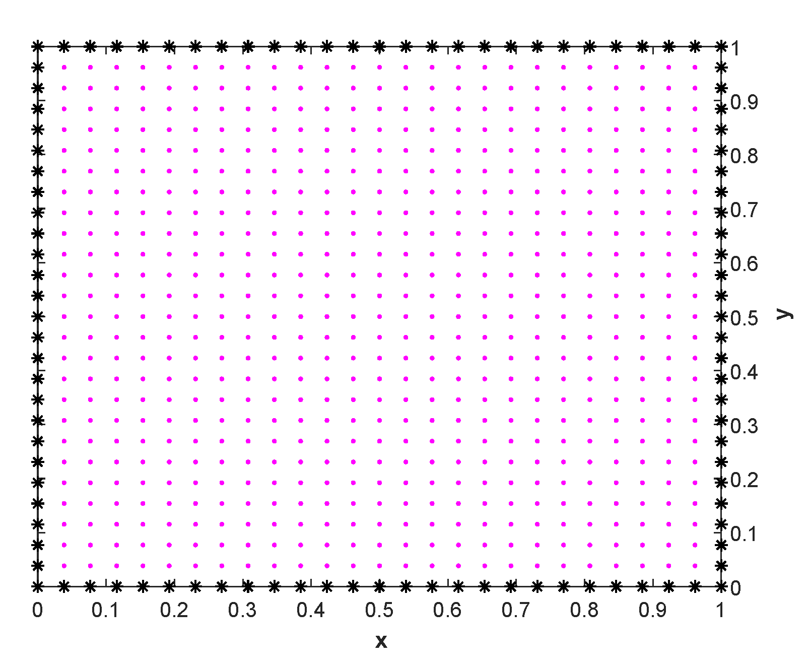
The proposed Laplace transform based local meshless method is tested on 2D linear multi-term FPIDEs. In our numerical experiments, we utilized the multiquadric (MQ) radial kernel defined by ϕ ( r , ε ) = 1 + ( ε r ) 2 . For the optimal shape parameter, the uncertainty principle due to [53] (e.g., in RBF methods, we cannot have both good accuracy and good conditioning at the same time) is utilized. We performed our experiments in MATLAB R2019a on a Windows 10(64 bit) PC equipped with an Intel(R) Core(TM) i5-3317U CPU @ 1.70 GHz and with 4 GB of RAM. We chose L = T = 1 , and d ρ = 1 , for ρ = 1 , 2 , 3 , , m . Let U ( ζ , τ ) be the exact solution and U k ( ζ , τ ) be the numerical solution. To validate the theoretical results, we used the L error defined as:
L = U ( ζ i , τ ) U k ( ζ i , τ ) = max 1 i N ( U ( ζ i , τ ) U k ( ζ i , τ ) ) .
In our numerical experiments, we consider the problem (1) with initial condition Θ = 0 , and the inhomogeneous term is given as:
f ( x , y , τ ) = Γ 9 5 τ 4 5 γ 1 Γ ( 9 5 γ 1 ) + τ 4 5 γ 2 Γ ( 9 5 γ 2 ) + 2 π 2 τ 4 5 + α Γ ( 9 5 + α ) sin ( π x ) sin ( π y ) .
The problem is solved with two types of boundary conditions, the Dirichlet boundary conditions generated from the exact solution given by:
U ( x , y , τ ) = τ 4 5 sin ( π x ) sin ( π y ) ,
and the Robin boundary conditions given as:
U ( x , y , τ ) + U ( x , y , τ ) · n = G ( x , y , τ ) , x , y Ω , τ [ 0 , 1 ] .
We solve the problem in the square domain, nut-shaped domain, and L-shaped domain.

6.1. Square Domain

In the first test, the problem is solved in square domain [ 0 , 1 ] 2 with Dirichlet boundary conditions. The domain is discretized with regularly distributed nodes, as shown in the Figure 1. Then, the proposed scheme is applied to the 2D multi-term FPIDE. The exact and approximate solutions of the problem are presented in Figure 2a,b. The computational results obtained for various points N Ω , n Ω i , and quadrature points M along the contour Γ are given in Table 1. The L error, shape parameter ε , error estimate, condition number κ , and the computational time (CPU (s)) are shown in Table 1. The obtained results ensure the efficiency and stability of the method.

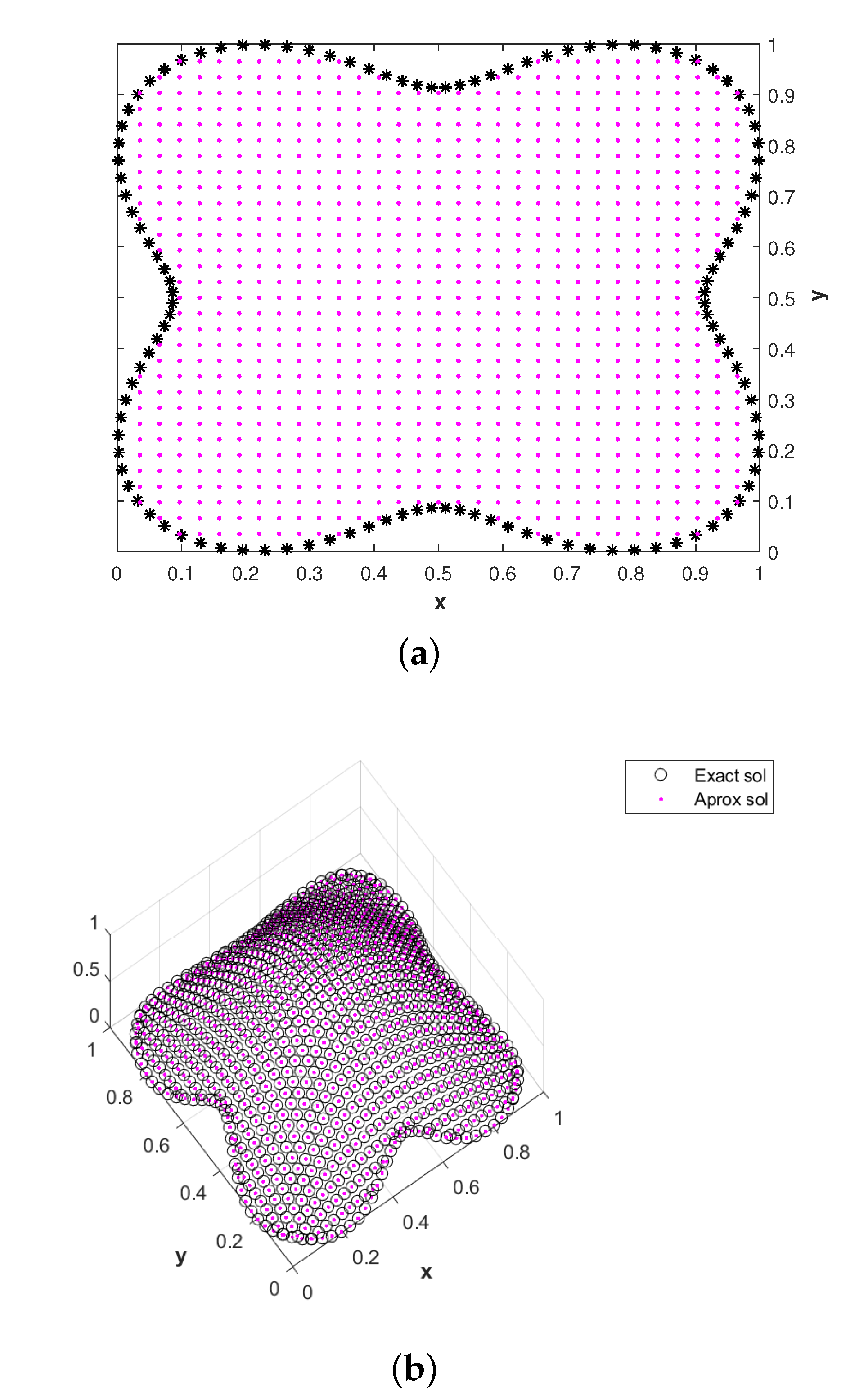
6.2. Nut-Shaped Domain

In the second test, the problem is solved in the nut-shaped domain with Dirichlet boundary conditions. The domain is discretized with regularly distributed nodes, as shown in the Figure 3a. Then, the proposed scheme is applied to the 2D multi-term FPIDE. The exact and the numerical solutions of the problem are presented in Figure 3b. The computational results obtained for various points N Ω , n Ω i , and quadrature points M along the contour Γ are shown in Table 2. The L error, shape parameter ε , error estimate, condition number κ , and the computational time (CPU (s)) are shown in Table 2. The obtained results ensure the efficiency of the proposed method for problems defined in irregular domains.

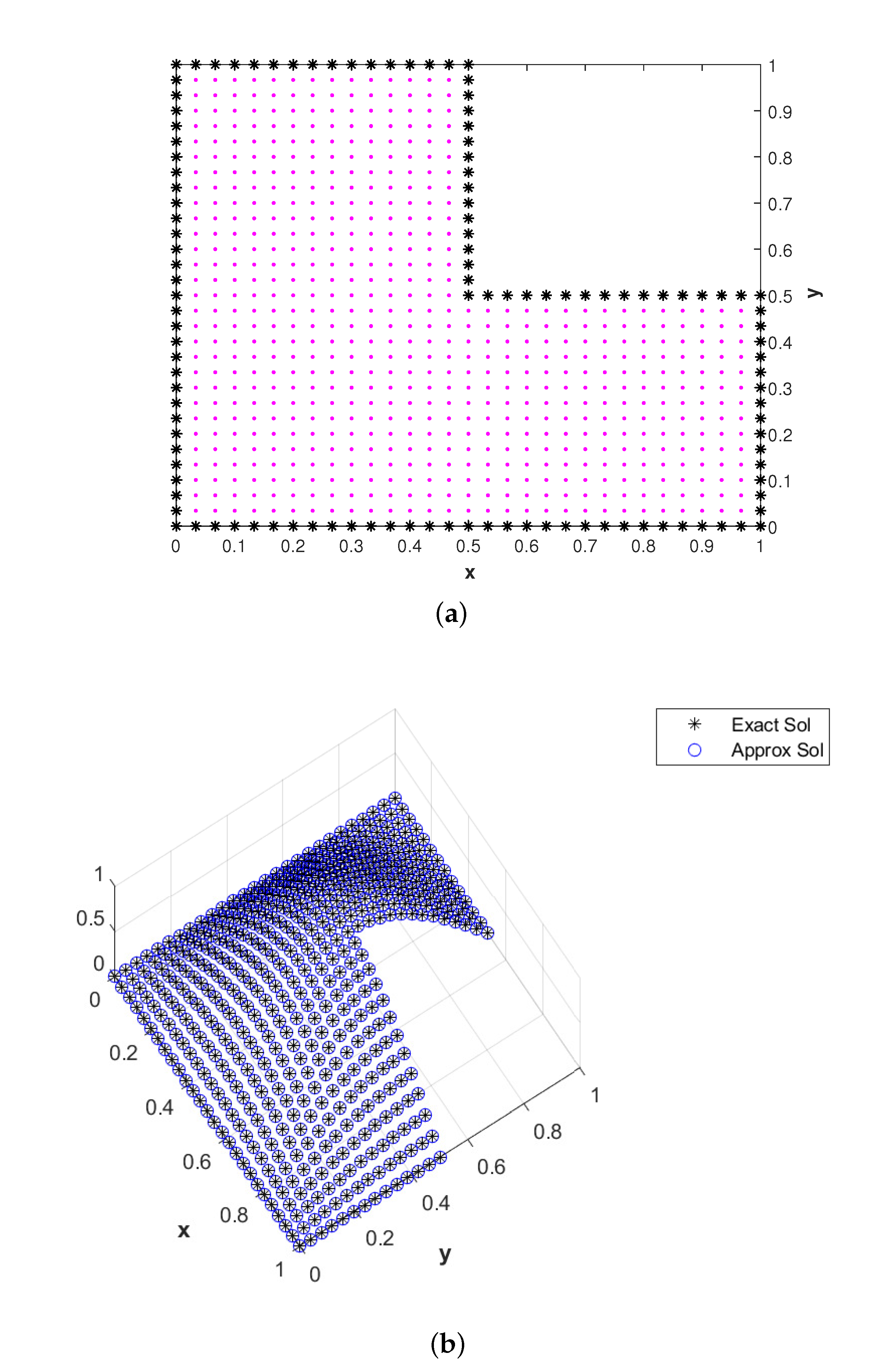
6.3. L-Shaped Domain

In the third test, the problem is solved in the L-shaped domain with Dirichlet and Robin boundary conditions. The domain is discretized with regularly distributed nodes, as shown in the Figure 4a. Then, the proposed method is applied to the 2D multi-term FPIDE. The exact and the numerical solutions of the problem are presented in Figure 4b. The computational results obtained for various points N Ω , n Ω i , and quadrature points M along the contour Γ with Dirichlet boundary conditions are shown in Table 3. The L error, shape parameter ε , error estimate, condition number κ , and the computational time (CPU (s)) are shown in Table 3. Figure 5 shows the absolute error obtained using Robin boundary conditions. The obtained results ensure the efficiency of the proposed method for problems defined in irregular domains.

7. Conclusions

We successfully coupled the Laplace transform and localized meshless method for the approximation of the solution of the multi-term 2D FPIDE. The time stepping procedure was avoided via the Laplace transform, and the issues arising due to dense differentiation matrices were resolved via the localized meshless method. For the contour integration, we utilized the recently introduced improved Talbot’s contour. The convergence and stability of the method were discussed. To validate the numerical scheme and check its efficiency, the numerical experiments were carried out in the square, nut-shaped, and L-shaped domains. From the results obtained, it was observed that the proposed numerical scheme is efficient and has better accuracy compared to other available work. It was observed that the improved Talbot’s method is computationally more useful than other available methods. The results led us to the conclusion that the proposed method is capable of solving FPIDEs without time instability in less computation time.

Author Contributions

Conceptualization, K. and Z.S.; Data curation, Z.S.; Funding acquisition, Z.S. and P.K.; Investigation, K. and Z.S.; Methodology, K., Z.S. and P.K.; Project administration, Z.S. and P.K.; Software, K. and N.A.A.; Supervision, Z.S.; Validation, Z.S., P.K. and N.A.A.; Visualization, N.A.A.; Writing—original draft, K.; Writing—review & editing, P.K. and N.A.A. All authors have read and agreed to the published version of the manuscript.

Funding

This research received no external funding.

Acknowledgments

The authors acknowledge the financial support provided by the Center of Excellence in Theoretical and Computational Science (TaCS-CoE), KMUTT.

Conflicts of Interest

The authors declare no conflict of interest.

References

  1. Renardy, M. Mathematical analysis of viscoelastic flows. Ann. Rev. Fluid Mech. 1989, 21, 21–36. [Google Scholar] [CrossRef]
  2. Al-Smadi, M.; Arqub, O.A. Computational algorithm for solving Fredholm time-fractional partial integro-differential equations of Dirichlet functions type with error estimates. Appl. Math. Comput. 2019, 342, 280–294. [Google Scholar]
  3. Arshed, S. B-spline solution of fractional integro partial differential equation with a weakly singular kernel. Numer. Methods Partial Differ. Equ. 2017, 33, 1565–1581. [Google Scholar] [CrossRef]
  4. Arqub, O.A.; Al-Smadi, M. Numerical algorithm for solving time-fractional partial integro-differential equations subject to initial and Dirichlet boundary conditions. Numer. Methods Partial Differ. Equ. 2018, 34, 1577–1597. [Google Scholar] [CrossRef]
  5. Tang, T. A finite difference scheme for partial integro-differential equations with a weakly singular kernel. Appl. Numer. Math. 1993, 11, 309–319. [Google Scholar] [CrossRef]
  6. Long, W.; Xu, D.; Zeng, X. Quasi wavelet based numerical method for a class of partial integro-differential equation. Appl. Math. Comput. 2012, 218, 11842–11850. [Google Scholar] [CrossRef]
  7. Chen, C.; Thome, V.; Wahlbin, L.B. Finite element approximation of a parabolic integro-differential equation with a weakly singular kernel. Math. Comput. 1992, 58, 587–602. [Google Scholar] [CrossRef]
  8. Xu, D. On the discretization in time for a parabolic integro-differential equation with a weakly singular kernel I: Smooth initial data. Appl. Math. Comput. 1993, 58, 1–27. [Google Scholar]
  9. Wulan, L.; Xu, D. Finite central difference/finite element approximations for parabolic integro-differential equations. Computing 2010, 90, 89–111. [Google Scholar]
  10. EL-Asyed, A.M.A.; Soliman, A.F.; El-Azab, M.S. On the numerical solution of partial integro-differential equations. Math. Sci. Lett. 2012, 1, 71–80. [Google Scholar]
  11. Fairweather, G. Spline collocation methods for a class of hyperbolic partial integro-differential equations. SIAM J. Numer. Anal. 1994, 31, 444–460. [Google Scholar] [CrossRef]
  12. Siddiqi, S.S.; Arshed, S. Cubic B-spline for the Numerical Solution of Parabolic Integro-differential Equation with a Weakly Singular Kernel. Res. J. Appl. Sci. Eng. Technol. 2014, 7, 2065–2073. [Google Scholar] [CrossRef]
  13. Huang, Y.Q. Time discretization scheme for an integro-differential equation of parabolic type. J. Comput. Math. 1994, 12, 259–263. [Google Scholar]
  14. Hu, S.; Qiu, W.; Chen, H. A backward Euler difference scheme for the integro-differential equations with the multi-term kernels. Int. J. Comput. Math. 2020, 97, 1254–1267. [Google Scholar] [CrossRef]
  15. Kılıçman, A.; Ahmood, W.A. Solving multi-dimensional fractional integro-differential equations with the initial and boundary conditions by using multi-dimensional Laplace Transform method. Tbilisi Math. J. 2017, 10, 105–115. [Google Scholar] [CrossRef]
  16. Gu, X.M.; Wu, S.L. A parallel-in-time iterative algorithm for Volterra partial integral-differential problems with weakly singular kernel. J. Comput. Phys. 2020, 417, 109576. [Google Scholar] [CrossRef]
  17. Saadatmandi, A.; Khani, A.; Azizi, M.R. A sinc-Gauss-Jacobi collocation method for solving Volterra’s population growth model with fractional order. Tbilisi Math. J. 2018, 11, 123–137. [Google Scholar] [CrossRef]
  18. Moradi, L.; Mohammadi, F.; Conte, D. A discrete orthogonal polynomials approach for coupled systems of nonlinear fractional order integro-differential equations. Tbilisi Math. J. 2019, 12, 21–38. [Google Scholar] [CrossRef]
  19. Alsaedi, A.; Agarwal, R.P.; Ntouyas, S.K.; Ahmad, B. Fractional-Order Integro-Differential Multivalued Problems with Fixed and Nonlocal Anti-Periodic Boundary Conditions. Mathematics 2020, 8, 1774. [Google Scholar] [CrossRef]
  20. Ahmad, B.; Broom, A.; Alsaedi, A.; Ntouyas, S.K. Nonlinear integro-differential equations involving mixed right and left fractional derivatives and integrals with nonlocal boundary data. Mathematics 2020, 8, 336. [Google Scholar] [CrossRef] [Green Version]
  21. Amin, R.; Nazir, S.; García-Magariño, I. A Collocation Method for Numerical Solution of Nonlinear Delay Integro-Differential Equations for Wireless Sensor Network and Internet of Things. Sensors 2020, 20, 1962. [Google Scholar] [CrossRef] [Green Version]
  22. Nemati, S.; Torres, D.F. Application of Bernoulli Polynomials for Solving Variable-Order Fractional Optimal Control-Affine Problems. Axioms 2020, 9, 114. [Google Scholar] [CrossRef]
  23. Holhos, A.; Rosca, D. Orhonormal wavelet bases on the 3D ball via volume preserving map from the regular octahedron. arXiv 2019, arXiv:1910.08067. [Google Scholar]
  24. Jäntschi, L. The eigenproblem translated for alignment of molecules. Symmetry 2019, 11, 1027. [Google Scholar] [CrossRef] [Green Version]
  25. Bazgir, H.; Ghazanfari, B. Existence of Solutions for Fractional Integro-Differential Equations with Non-Local Boundary Conditions. Math. Comput. Appl. 2018, 23, 36. [Google Scholar] [CrossRef] [Green Version]
  26. Georgieva, A. Double Fuzzy Sumudu Transform to Solve Partial Volterra Fuzzy Integro-Differential Equations. Mathematics 2020, 8, 692. [Google Scholar] [CrossRef]
  27. Biazar, J.; Asadi, M.A. FD-RBF for partial integro-differential equations with a weakly singular kernel. Appl. Comput. Math. 2015, 4, 445–451. [Google Scholar] [CrossRef] [Green Version]
  28. Ali, G.; Gómez-Aguilar, J.F. Approximation of partial integro differential equations with a weakly singular kernel using local meshless method. Alex. Eng. J. 2020, 59, 2091–2100. [Google Scholar] [CrossRef]
  29. Aslefallah, M.; Shivanian, E. A nonlinear partial integro-differential equation arising in population dynamic via radial basis functions and theta-method. J. Math. Comput. Sci. 2014, 13, 14–25. [Google Scholar] [CrossRef] [Green Version]
  30. Safinejad, M.; Moghaddam, M.M. A local meshless RBF method for solving fractional integro-differential equations with optimal shape parameters. Ital. J. Pure Appl. Math. 2019, 41, 382. [Google Scholar]
  31. Fu, Z.J.; Chen, W.; Yang, H.T. Boundary particle method for Laplace transformed time fractional diffusion equations. J. Comput. Phys. 2013, 235, 52–66. [Google Scholar] [CrossRef]
  32. Davies, A.J.; Crann, D.; Mushtaq, J. A parallel implementation of the Laplace transform BEM. WIT Trans. Model. Simul. 1970, 14. [Google Scholar] [CrossRef]
  33. Gia, Q.T.L.; Mclean, W. Solving the heat equation on the unit sphere via Laplace transforms and radial basis functions. Adv. Comput. Math. 2014, 40, 353–375. [Google Scholar] [CrossRef] [Green Version]
  34. McLean, W.; Thomee, V. Numerical solution via Laplace transforms of a fractional order evolution equation. J. Integral Equ. Appl. 2010, 22, 57–94. [Google Scholar] [CrossRef]
  35. Fernandez, M.L.; Palencia, C. On the numerical inversion of the Laplace transform of certain holomorphic mappings. Appl. Numer. Math. 2004, 51, 289–303. [Google Scholar] [CrossRef]
  36. Jacobs, B.A. High-order compact finite difference and Laplace transform method for the solution of time fractional heat equations with Dirichlet and Neumann boundary conditions. Numer. Methods Partial Differ. Equ. 2016, 32, 1184–1199. [Google Scholar] [CrossRef]
  37. Li, X.; Haq, A.U.; Zhang, X. Numerical solution of the linear time fractional Klein-Gordon equation using transform based localized RBF method and quadrature. AIMS Math. 2020, 5, 5287–5308. [Google Scholar] [CrossRef]
  38. Uddin, M.; Ali, A. A localized transform-based meshless method for solving time fractional wave-diffusion equation. Eng. Anal. Bound. Elem. 2018, 92, 108–113. [Google Scholar] [CrossRef]
  39. Li, J.; Dai, L.; Nazeer, W. Numerical solution of multi-term time fractional wave diffusion equation using transform based local meshless method and quadrature. AIMS Math. 2020, 5, 5813–5838. [Google Scholar] [CrossRef]
  40. Zhou, J.; Xu, D. Alternating direction implicit difference scheme for the multi-term time-fractional integro-differential equation with a weakly singular kernel. Comput. Math. Appl. 2020, 79, 244–255. [Google Scholar] [CrossRef]
  41. Oldham, K.B.; Spanier, J. The Fractional Calculus Theory and Applications of Differentiation and Integration to Arbitrary Order; Academic Press: New York, NY, USA; London, UK, 1974; Volume 111. [Google Scholar]
  42. Podlubny, I. Fractional Differential Equations. In Mathematics in Science and Engineering; Elsevier: Amsterdam, The Netherlands, 1999; Volume 198. [Google Scholar]
  43. Popolizio, M. Numerical solution of multiterm fractional differential equations using the matrix Mittag-Leffler functions. Mathematics 2018, 6, 7. [Google Scholar] [CrossRef] [Green Version]
  44. Schiessel, H.; Metzler, R.; Blumen, A.; Nonnenmacher, T.F. Generalized viscoelastic models: Their fractional equations with solutions. J. Phys. A Math. Gen. 1995, 28, 6567. [Google Scholar] [CrossRef]
  45. Torvik, P.J.; Bagley, R.L. On the appearance of the fractional derivative in the behavior of real materials. J. Appl. Mech. 1984, 51, 294–298. [Google Scholar] [CrossRef]
  46. Qin, S.; Liu, F.; Turner, I.; Vegh, V.; Yu, Q.; Yang, Q. Multi-term time-fractional Bloch equations and application in magnetic resonance imaging. J. Comput. Appl. Math. 2017, 319, 308–319. [Google Scholar] [CrossRef] [Green Version]
  47. Diethelm, K. The Analysis of Fractional Differential Equations: An Application-Oriented Exposition Using Differential Operators of Caputo Type; Springer Science & Business Media: Berlin, Germany, 2010. [Google Scholar]
  48. Šarler, B.; Vertnik, R. Meshfree explicit local radial basis function collocation method for diffusion problems. Comput. Math. Appl. 2006, 51, 1269–1282. [Google Scholar] [CrossRef] [Green Version]
  49. Talbot, A. The accurate numerical inversion of Laplace transform. J. Inst. Math. Appl. 1979, 23, 97–120. [Google Scholar] [CrossRef]
  50. Dingfelder, B.; Weideman, J.A.C. An improved Talbot method for numerical Laplace transform inversion. Numer. Algorithms 2015, 68, 167–183. [Google Scholar] [CrossRef] [Green Version]
  51. Weideman, J.A.C. Optimizing Talbot’s contours for the inversion of the Laplace transform. SIAM J. Numer. Anal. 2006, 44, 2342–2362. [Google Scholar] [CrossRef] [Green Version]
  52. Sarra, S.A.; Kansa, E.J. Multiquadric radial basis function approximation methods for the numerical solution of partial differential equations. Adv. Comput. Mech. 2009, 2. [Google Scholar]
  53. Schaback, R. Error estimates and condition numbers for radial basis function interpolation. Adv. Comput. Math. 1995, 3, 251–264. [Google Scholar] [CrossRef]
Figure 1. Node distribution in the square domain.
Mathematics 08 01972 g001
Figure 2. (a) The exact solution in the square domain; (b) the numerical solution in the square domain.
Mathematics 08 01972 g002
Figure 3. (a) Node distribution in the nut-shaped domain; (b) the exact and numerical solutions in the nut-shaped domain.
Mathematics 08 01972 g003
Figure 4. (a) Nodes in the L-shaped domain; (b) the exact and numerical solutions in the L-shaped domain.
Mathematics 08 01972 g004
Figure 5. Absolute error using Robin boundary conditions in the L-shaped domain, with α = 0.5 , γ 1 = 0.75 , γ 2 = 0.95 , N = 736 , n = 73 , and M = 20 .
Mathematics 08 01972 g005
Table 1. Numerical results for the fractional partial integro-differential equations (FPIDEs) in the square domain.
NnM L ErrorError Estimate ε κ CPU(s)
α = 0.25 102473101.90 × 10 3 1.26 × 10 6 4.91.54 × 10 12 7.395020
γ 1 = 0.15 121.00 × 10 3 8.37 × 10 8 4.91.54 × 10 12 7.022358
γ 2 = 0.3 149.94 × 10 4 5.53 × 10 9 4.91.54 × 10 12 7.249688
169.91 × 10 4 3.66 × 10 10 4.91.54 × 10 12 7.789044
189.91 × 10 4 2.42 × 10 11 4.91.54 × 10 12 8.160190
α = 0.5 30202.20 × 10 3 1.60 × 10 12 3.31.40 × 10 12 6.398152
γ 1 = 0.45 40 3.70 × 10 3 1.60 × 10 12 4.01.69 × 10 12 6.328329
γ 2 = 0.55 50 2.0 × 10 3 1.60 × 10 12 4.41.56 × 10 12 7.150031
60 1.60 × 10 3 1.60 × 10 12 4.71.31 × 10 12 7.898109
70 1.60 × 10 3 1.60 × 10 12 4.82.10 × 10 12 8.372011
α = 0.75 72974221.10 × 10 3 1.05 × 10 13 4.11.64 × 10 12 5.758024
γ 1 = 0.65 841 9.04 × 10 4 1.05 × 10 13 4.51.16 × 10 12 6.988687
γ 2 = 0.75 961 8.75 × 10 4 1.05 × 10 13 4.81.26 × 10 12 10.074941
1089 1.70 × 10 3 1.05 × 10 13 5.11.35 × 10 12 10.822728
1225 8.47 × 10 4 1.05 × 10 13 5.41.44 × 10 12 13.236204
[40] 7.16 × 10 4
Table 2. Numerical results for the FPIDEs in nut-shaped domain.
NnM L ErrorError Estimate ε κ CPU (s)
α = 0.25 102476101.30 × 10 3 1.26 × 10 6 4.91.59 × 10 13 6.665154
γ 1 = 0.15 122.71 × 10 4 8.37 × 10 8 4.91.59 × 10 13 7.059290
γ 2 = 0.30 142.68 × 10 4 5.53 × 10 9 4.91.59 × 10 13 7.597790
162.69 × 10 4 3.66 × 10 10 4.91.59 × 10 13 8.066648
182.69 × 10 4 2.42 × 10 11 4.91.59 × 10 13 8.368624
α = 0.5 30201.13 × 10 2 1.60 × 10 12 3.28.99 × 10 13 6.499886
α = 0.55 40 1.90 × 10 3 1.60 × 10 12 3.85.33 × 10 13 7.088308
α = 0.65 50 1.30 × 10 3 1.60 × 10 12 4.32.31 × 10 13 6.949834
60 1.70 × 10 3 1.60 × 10 12 4.61.68 × 10 13 7.556786
74 7.44 × 10 4 1.60 × 10 12 4.91.24 × 10 13 9.184561
α = 0.75 97375225.37 × 10 4 1.05 × 10 13 5.01.09 × 10 12 8.624205
γ 1 = 0.75 983 2.48 × 10 4 1.05 × 10 13 4.91.76 × 10 12 9.407931
γ 2 = 0.90 993 5.54 × 10 4 1.05 × 10 13 5.02.12 × 10 12 9.242420
1003 5.62 × 10 4 1.05 × 10 13 4.95.40 × 10 12 9.108576
1013 5.39 × 10 4 1.05 × 10 13 4.91.21 × 10 13 9.380810
[40] 7.16 × 10 4
Table 3. Numerical results for the FPIDEs in the L-shaped domain.
NnM L ErrorError Estimate ε κ CPU (s)
α = 0.25 104575102.00 × 10 3 1.26 × 10 6 5.44.22 × 10 12 7.879603
γ 1 = 0.15 129.70 × 10 4 8.37 × 10 8 5.44.22 × 10 12 8.472794
γ 2 = 0.30 149.07 × 10 4 5.53 × 10 9 5.44.22 × 10 12 8.961569
169.03 × 10 4 3.66 × 10 10 5.44.22 × 10 12 9.776831
189.02 × 10 4 2.42 × 10 11 5.44.22 × 10 12 9.703955
α = 0.5 30201.20 × 10 3 1.60 × 10 12 3.46.85 × 10 12 6.230811
γ 1 = 0.45 40 1.70 × 10 3 1.60 × 10 12 4.28.39 × 10 12 7.051659
γ 1 = 0.55 50 7.94 × 10 4 1.60 × 10 12 4.84.53 × 10 12 7.786541
60 8.99 × 10 4 1.60 × 10 12 5.23.21 × 10 12 8.323130
72 7.80 × 10 4 1.60 × 10 12 5.43.98 × 10 12 9.694111
α = 0.75 73673227.68 × 10 4 1.05 × 10 13 4.54.06 × 10 12 5.941242
γ 1 = 0.75 833 8.30 × 10 4 1.05 × 10 13 4.84.06 × 10 12 7.343621
γ 1 = 0.85 936 6.45 × 10 4 1.05 × 10 13 5.14.06 × 10 12 8.402310
1045 7.49 × 10 4 1.05 × 10 13 5.44.06 × 10 12 10.279795
[40] 7.16 × 10 4
Publisher’s Note: MDPI stays neutral with regard to jurisdictional claims in published maps and institutional affiliations.

