Boundary Control for a Certain Class of Reaction-Advection-Diffusion System

Abstract

There are physical phenomena, involving diffusion and structural vibrations, modeled by partial differential equations (PDEs) whose solution reflects their spatial distribution. Systems whose dynamics evolve on an infinite-dimensional Hilbert space, i.e., infinite-dimensional systems, are modeled by PDEs. The aim when designing a controller for infinite-dimensional systems is similar to that for finite-dimensional systems, i.e., the control system must be stable. Another common goal is to design the controller in such a way that the response of the system does not be affected by external disturbances. The controller design for finite-dimensional systems is not an easy task, so, the controller design for infinite-dimensional systems is even more challenging. The backstepping control approach is a dominant methodology for boundary feedback design. In this work, we try with the backstepping design for the boundary control of a reaction-advection-diffusion (R-A-D) equation, namely, a type parabolic PDE, but with constant coefficients and Neumann boundary conditions, with actuation in one of these latter. The heat equation with Neumann boundary conditions is considered as the target system. Dynamics of the open- and closed-loop solution of the PDE system are validated via numerical simulation. The MATLAB${}^{\circledR }$-based numerical algorithm related with the implementation of the control scheme is here included.

1. Introduction

There are a large number of dynamic systems that can be modeled by partial differential equations (PDEs). Many of these systems can be found in the study of mechanical, electrical, or civil engineering as well as in the study of physics and chemistry sciences since all these disciplines deal with the study of fluid flow, heat transfer, electromagnetic field, beam deflection, acoustics, and many other physical phenomena. In the study of health and social sciences, PDEs can also be used to model spread of diseases and viruses as well as population growth. One of the main features of the phenomena mentioned above is that these are listed as distributed parameters systems (DPSs), which are characterized by having two or more independent variables where the combination of one spatial variable with one temporal variable is the most common. Another feature from the DPSs is that these are infinite-dimensional systems. PDEs can be categorized as of parabolic type, elliptic type and hyperbolic type. Each one of these categories describes the behavior of different phenomena, e.g., parabolic PDEs are mainly used to describe heat transfer systems and diffusion systems, elliptic PDEs are used to describe steady state behavior for systems such as electrostatic fields, and hyperbolic PDEs are associated with vibration or wave phenomena. To get the general solution (dynamics) from a PDE system, it is necessary to set not only initial conditions but boundary conditions which can be from three types, namely, the so-called Dirichlet, Neumann, and Robin conditions [1].

From control theory, the backstepping methodology can be used to force a finite-dimensional nonlinear dynamical system, mainly modeled by ordinary differential equations (ODEs), to behave like a linear system in a new set of coordinates [2,3]. The backstepping methodology has been extended from control of finite-dimensional ODEs systems to control of infinite-dimensional PDEs systems. Control of PDEs systems can be performed in two ways, depending on the location of sensors and actuators, either in the domain dimension or at the boundary.

One of the first attempts about backstepping control design for linear parabolic PDEs was reported in [4]. The backstepping methodology applied to the boundary control of PDEs, from considering Dirichlet and Neumann boundary value problems on the control of an unstable heat equation, was introduced in [5]. In [6], from the structure for a class of one-dimensional (1-D) linear parabolic partial integro-differential equations (P(I)DEs), with one Neumann boundary condition and control signal applied through either Dirichlet and Neumann boundary actuation, the backstepping methodology was used to establish an explicit expression for the gain kernel, namely the gain kernel P(I)DE system, of the boundary control law. Furthermore, the backstepping approach was extended to the design of inverse optimal controllers. From the gain kernel, explicit solutions for the boundary state feedback laws to the control of an unstable heat equation, a heat equation with destabilizing boundary condition, a reaction-diffusion (R-D) equation with spatially varying coefficient for the reaction term, and for a solid propellant rocket model, were obtained. In [7], the backstepping methodology was translated to the design of state observers with boundary sensing. Adaptive boundary controllers for parabolic PDEs were derived in [8,9,10,11]. The adaptive approaches were extended to reaction-advection-diffusion (R-A-D) systems in higher dimensions (2-D and 3-D) and to systems with spatially varying unknown parameters [12,13]. Most of the work cited above was compiled in [12,14]. Adaptive control of linear hyperbolic PDEs following the backstepping (Volterra integral transformation) strategy can be found in [15]. Furthermore, through the use of Volterra and Fredholm integral transformations, the input-to-state stability (ISS) approach has been extended to the control of 1-D PDEs in [16].

Boundary control design for a R-A-D equation via backstepping approach seems like a challenging task. Because of the inclusion of partial derivatives in its structure, the searching for the solution of the gain kernel PDE represents a tedious work when trying with the solution for an integral equation equivalent to the kernel PDE. In our work, we focus our attention in the design of a Neumann stabilizing controller for a R-A-D equation, namely, a linear parabolic PDE, but with constant coefficients and Neumann boundary conditions, with actuation in one of these latter. A heat equation with Neumann boundary conditions is considered as target system. This work is motivated from [14], where the Neumann stabilizing controller design to this class of PDE system is left as an exercise to the reader.

The manuscript is summarized as follows. The description of functions spaces is given in Section 2. In Section 3, the R-A-D PDE with constant parameters and boundary conditions of the Neumann type is shown. The R-A-D equation is reduced through a proper change of variables to a R-D system in order to implement the backstepping methodology for boundary control. In Section 4, once that the original system has been reduced to the form of a R-D equation, a target system is proposed in order to, invoking the Lyapunov approach, guarantee exponential stability. In Section 5, the main idea of the backstepping approach, a Volterra integral transformation in order to map the original PDE system into a reduced one, namely, the target system, is applied. As a result, a new PDE system is obtained in function of the so-called kernel gain. Then, by a change of variables, the solution for the integral equation is obtained. By using the successive approximations method for integral equations, as a result, the value of the kernel gain is obtained at Section 6. Once the kernel gain value is obtained, in Section 7 we back to the original variables getting so the stabilizing controller to be implemented on the boundary actuated from the original system. In Section 8, the numerical algorithm used here, in order to implement and replicate our work, is given. Simulation results are discussed at Section 9. Conclusions are drawn at the end of the paper.

2. Function Spaces

Let us denote by $\Omega$ an open set of ${\mathbb{R}}^n$ with boundary $\Gamma$. Let us assume that either $\Omega$ is Lipschitz or $\Omega$ is of class $C^r$ for $r\ge 1$. The generic point of ${\mathbb{R}}^n$ is denoted by $x=\{x_1,\dots ,x_n\}$. The Lebesgue measure on ${\mathbb{R}}^n$ is denoted by $dx=d{x}_1\dots d{x}_n$.

Let us denote by $C(\Omega )$ (resp. $C^k(\Omega ),k\in \mathbb{N}$ or $k=\infty$) the space of real continuous functions on $\Omega$ (resp. the space of k times continuously differentiable functions on $\Omega$), $C\left(\overline{\Omega }\right)$ (resp. $C^k\left(\overline{\Omega }\right)$) represents the space of real continuous functions on $\overline{\Omega }$ (resp. the space of k times continuously differentiable functions on $\Omega$). The spaces of real $C^{\infty }$ functions on $\Omega$ with a compact support in $\Omega$ are denoted by $C_0^{\infty }$.

For $p\in [1,\infty )$, $L^p(\Omega )$ is the space of real functions on $\Omega$ which are $L^p$ for the Lebesgue measure. It is a Banach space for the norm

$${\parallel u\parallel }_{L^p(\Omega )}={\left({\int }_{\Omega }{\left|u\left(x\right)\right|}^{p}dx\right)}^{1/p}.$$

(1)

For $p=\infty$, $L^{\infty }(\Omega )$ is the space of measurable and bounded real functions on $\Omega$. It is also a Banach space for the norm

$${\parallel u\parallel }_{L^{\infty }(\Omega )}=\mathrm{ess}{\sup }_{x\in \Omega }\left|u\left(x\right)\right|.$$

(2)

For $p=2$, $L^2(\Omega )$ is a Hilbert space for the scalar product

$$(u,v)={\int }_{\Omega }u\left(x\right)·v\left(x\right)dx$$

(3)

with the corresponding norm denoted by

$$\mid u\mid ={\parallel u\parallel }_{L^2(\Omega )}={\left\{(u,u)\right\}}^{1/2}.$$

(4)

Let us denote by $W^{s,p}(\Omega )$, $s\in \mathbb{N},p\in [1,\infty ]$, the Sobolev space of functions u in $L^p(\Omega )$ whose distribution derivatives of order less than or equal to s are in $L^p(\Omega )$. It is a Banach space for the norm

$${\parallel u\parallel }_{W^{s,p}(\Omega )}=\sum _{\left[\alpha \right]\le s}{\parallel D^{\alpha }u\parallel }_{L^p(\Omega )}$$

(5)

where $D_{i}u=\partial u/\partial x_i$, $i\in [1,n]$, is the notation for the partial differential derivatives of a function u, $D^{\alpha }u=D_1^{{\alpha }_1}\dots D_n^{{\alpha }_n}u=\left({\partial }^{{\alpha }_1+\cdots +{\alpha }_n}u\right)/(\partial x_1^{{\alpha }_1}\dots \partial x_n^{{\alpha }_n})$, $\alpha =\{{\alpha }_1,\dots ,{\alpha }_n\}\in {\mathbb{N}}^n$, and $\left[\alpha \right]={\alpha }_1+\cdots +{\alpha }_n$. For $p=2$, $W^{s,2}(\Omega )=H^s(\Omega )$ and this is a Hilbert space for the scalar product

$${\left((u,v)\right)}_{H^s(\Omega )}=\sum _{\left[\alpha \right]\le s}(D^{\alpha }u,D^{\alpha }v).$$

(6)

Let us consider the Sobolev spaces $H^s(\Omega )$ which contain $C^{\infty }\left(\overline{\Omega }\right)$ and $C^s\left(\overline{\Omega }\right)$. The closure of $C_0^{\infty }(\Omega )$ in $H^s(\Omega )$ (resp. $W^{s,p}(\Omega )$) is denoted by $H_0^s(\Omega )$ (resp. $W_0^{s,p}(\Omega )$). In particular,

$$\begin{array}{ccc}\hfill H^1(\Omega )& =& \{u\in L^2(\Omega ),D_{i}u\in L^2(\Omega ),1\le i\le n\},\hfill \end{array}$$

(7)

$$\begin{array}{ccc}\hfill H_0^1(\Omega )& =& \mathrm{the}\mathrm{closure}\mathrm{of}{C}_0^{\infty }(\Omega )\mathrm{in}{H}^1(\Omega ),\hfill \end{array}$$

(8)

which are Hilbert spaces for the scalar product

$${\left((u,v)\right)}_{H^1(\Omega )}=(u,v)+\sum _{i=1}^n(D_{i}u,D_{i}v).$$

(9)

For a bounded $\Omega$, the Poincaré inequality

$$\left|u\right|\le c_0(\Omega ){\left\{\sum _{i=1}^n{\left|D_{i}u\right|}^2\right\}}^{1/2},\forall u\in H_0^1(\Omega ),$$

(10)

implies that $H_0^1(\Omega )$ is a Hilbert space for the scalar product

$$\left((u,v)\right)=\sum _{i=1}^n(D_{i}u,D_{i}v)$$

(11)

and that the corresponding norm

$$\parallel u\parallel ={\left\{\left((u,u)\right)\right\}}^{1/2}$$

(12)

is equivalent to the norm induced by $H^1(\Omega )$ [17].

3. Reaction-Advection-Diffusion (R-A-D) System

In order to show how to apply the backstepping methodology to the boundary control of a certain class of R-A-D system, we will illustrate the procedure that must be systematically followed to reach the goal.

Let us consider a R-A-D system of the form

$$\begin{array}{cc}\hfill u_t(x,t)& =u_{xx}(x,t)+b{u}_x(x,t)+\lambda u(x,t),\hfill \end{array}$$

(13)

$$\begin{array}{cc}\hfill u_x(0,t)& =-\frac{b}{2}u(0,t),\hfill \end{array}$$

(14)

$$\begin{array}{cc}\hfill u_x(1,t)& =\mathcal{U}\left(t\right),\hfill \end{array}$$

(15)

for a function $u(x,t)$ defined in the spatial variable $x\in [0,1]$ and time $t\in [0,\infty )$, b and $\lambda$ are arbitrary constant coefficients, $\mathcal{U}\left(t\right)$ is the actuation signal (Neumann actuation) and Neumann boundary conditions are imposed. $u_{xx}(x,t)$ is the diffusion term, $b{u}_x(x,t)$ is the advection term, and $\lambda u(x,t)$ is the reaction term. First of all, let us consider the following change of variables

$$\begin{array}{cc}\hfill v(x,t)& =u(x,t)e^{(b/2)x}\hfill \end{array}$$

(16)

in order to eliminate the advection term $u_x(x,t)$. To do this, we calculate the temporal derivative from (16) which results

$$\begin{array}{cc}\hfill u_t(x,t)& =v_t(x,t)e^{-(b/2)x}.\hfill \end{array}$$

(17)

Now, calculating the spatial derivatives from (16) these are given by

$$\begin{array}{cc}\hfill u_x(x,t)& =v_x(x,t)e^{-(b/2)x}-\frac{b}{2}v(x,t)e^{-(b/2)x},\hfill \end{array}$$

(18)

$$\begin{array}{cc}\hfill u_{xx}(x,t)& =v_{xx}(x,t)e^{-(b/2)x}-b{v}_x(x,t)e^{-(b/2)x}+{\left(\frac{b}{2}\right)}^{2}v(x,t)e^{-(b/2)x}.\hfill \end{array}$$

(19)

Then, the R-A-D Equation (13) becomes

$$\begin{array}{cc}\hfill v_t(x,t)& =v_{xx}(x,t)+{\lambda }_{0}v(x,t)\hfill \end{array}$$

(20)

with ${\lambda }_0=\lambda -\frac{b^2}{4}$. Next, the boundary conditions are calculated by deriving (16), so,

$$\begin{array}{cc}\hfill v_x(x,t)& =u_x(x,t)e^{(b/2)x}+\frac{b}{2}u(x,t)e^{(b/2)x}\hfill \end{array}$$

(21)

which evaluated at the boundary $x=0$ it results

$$\begin{array}{cc}\hfill v_x(0,t)& =u_x(0,t)+\frac{b}{2}u(0,t).\hfill \end{array}$$

From (14),

$$\begin{array}{cc}\hfill v_x(0,t)& =-\frac{b}{2}u(0,t)+\frac{b}{2}u(0,t)\hfill \\ \hfill & =0.\hfill \end{array}$$

(22)

Now, evaluating (21) for $x=1$ we get

$$\begin{array}{cc}\hfill v_x(1,t)& =u_x(1,t)e^{b/2}+\frac{b}{2}u(1,t)e^{b/2}.\hfill \end{array}$$

(23)

In this way, we have obtained (20) as a reduced model from (13) given in the form of a R-D equation with boundary conditions (22) and (23).

4. Target System

At this point, we must define through a target system the desirable dynamics to be described by (20) in order to that it will behave like a stable system. A R-D system with negative magnitude to the reaction term can be a good choice as an exponentially stable one [5,12]. However, let us consider the heat equation

$$\begin{array}{cc}\hfill w_t(x,t)& =w_{xx}(x,t),\hfill \end{array}$$

(24)

$$\begin{array}{cc}\hfill w_x(0,t)& =0,\hfill \end{array}$$

(25)

$$\begin{array}{cc}\hfill w_x(1,t)& =-\frac{1}{2}w(1,t),\hfill \end{array}$$

(26)

as target system, as it is usual in boundary control of PDEs [14] due to its physical motivation [4], but with Neumann boundary conditions for a function $w(x,t)$ defined in the spatial variable $x\in [0,1]$ and time $t\in [0,\infty )$. In the following, we must prove that the target system (24)–(26) is exponentially stable in the sense of the $L_2$-norm of the state $w(x,t)$ with respect to the spatial variable limited to the unit domain. The $L_2$-norm is defined by

$$\begin{array}{cc}\hfill \parallel w(x,t)\parallel & ={\left({\int }_0^1{w}^2(x,t)dx\right)}^{1/2}.\hfill \end{array}$$

(27)

Let us consider the Lyapunov function

$$\begin{array}{cc}\hfill V(x,t)& =\frac{1}{2}{\int }_0^1{w}^2(x,t)dx,\hfill \end{array}$$

(28)

whose time derivative is given by

$$\begin{array}{cc}\hfill \dot{V}(x,t)& =\frac{dV}{dt}={\int }_0^{1}w(x,t)w_t(x,t)dx.\hfill \end{array}$$

(29)

From (24), the time derivative $\dot{V}$ of V can be rewritten as

$$\begin{array}{cc}\hfill \dot{V}(x,t)& ={\int }_0^{1}w(x,t)w_{xx}(x,t)dx.\hfill \end{array}$$

(30)

By using integration by parts we obtain

$$\begin{array}{cc}\hfill \dot{V}(x,t)& =w(1,t)w_x(1,t)-w(0,t)w_x(0,t)-{\int }_0^1{w}_x^2(x,t)dx,\hfill \end{array}$$

from which taking into account the boundary conditions (25) and (26) results

$$\begin{array}{cc}\hfill \dot{V}(x,t)& =-\frac{1}{2}{w}^2(1,t)-{\int }_0^1{w}_x^2(x,t)dx.\hfill \end{array}$$

(31)

In order to continue with our analysis, the following lemma which establishes the relationship between the $L_2$-norms of $w(x,t)$ and $w_x(x,t)$ will be of utility.

Lemma 1

(Poincaré Inequality). [12] For any $w\in H^1(0,1)$ (Sobolev space) the following inequalities hold

$$\begin{array}{c}\hfill \begin{array}{cc}\hfill {\int }_0^1{w}^2(x,t)dx& \le 2w^2(1,t)+4{\int }_0^1{w}_x^2(x,t)dx,\hfill \\ \hfill {\int }_0^1{w}^2(x,t)dx& \le 2w^2(0,t)+4{\int }_0^1{w}_x^2(x,t)dx.\hfill \end{array}\end{array}$$

(32)

Proof. 

See [12].

Multiplying both sides of (31) by a constant we get

$$\begin{array}{cc}\hfill 4\dot{V}(x,t)& =-2w^2(1,t)-4{\int }_0^1{w}_x^2(x,t)dx.\hfill \end{array}$$

(33)

From Lemma 1, this last identity can be written as

$$\begin{array}{cc}\hfill \dot{V}(x,t)& \le -\frac{1}{4}{\int }_0^1{w}^2(x,t)dx,\hfill \end{array}$$

(34)

which, considering (28), can be rewritten as

$$\begin{array}{cc}\hfill \dot{V}(x,t)& \le -\frac{1}{2}V(x,t).\hfill \end{array}$$

(35)

Let us try to solve this last relation by integration, where (35) can be equivalently written as

$$\begin{array}{cc}\hfill \frac{d\left(V\right(x,t\left)\right)}{dt}& \le -\frac{1}{2}V(x,t).\hfill \end{array}$$

So, separating variables and considering the integral symbol we get

$$\begin{array}{cc}\hfill \int \frac{d\left(V\right(x,t\left)\right)}{V(x,t)}& \le -\frac{1}{2}\int dt.\hfill \end{array}$$

Then, solving each integral it yields

$$\begin{array}{cc}\hfill ln\left(V\right(x,t\left)\right)& \le -\frac{1}{2}t+c.\hfill \end{array}$$

Since the natural logarithm $ln\left(x\right)$ is defined as the inverse function to the exponential function $e^x$, this last inequality can be expressed by

$$\begin{array}{cc}\hfill e^{ln\left(V\right(x,t\left)\right)}& \le e^{-(1/2)t}{e}^c,\hfill \end{array}$$

i.e.,

$$\begin{array}{cc}\hfill V(x,t)& \le e^{-(1/2)t}{e}^c,\hfill \end{array}$$

(36)

from which, setting $t=0$ results

$$\begin{array}{cc}\hfill V(x,0)& \le e^c.\hfill \end{array}$$

(37)

Additionally, we need to prove that $V(x,t)\le V(x,0)$ in order to guarantee that the Lyapunov function is bounded. So, from the definition for which is desirable that $\dot{V}(x,t)$ be negative semidefinite, i.e.,

$$\dot{V}(x,t)\le 0,$$

(38)

integrating both sides from such inequality, i.e.,

$$\begin{array}{cc}\hfill {\int }_0^t\dot{V}(x,t)dt& \le 0{\int }_0^{t}dt,\hfill \end{array}$$

and evaluating limits, it results

$$\begin{array}{cc}\hfill V(x,t)-V(x,0)& \le 0.\hfill \end{array}$$

Consequently,

$$\begin{array}{cc}\hfill V(x,t)& \le V(x,0).\hfill \end{array}$$

Thus, from (36)

$$\begin{array}{cc}\hfill V(x,t)& \le V(x,0)e^{-(1/2)t},\hfill \end{array}$$

(39)

or, by using (28) in terms of the $L_2$-norm (27),

$$\begin{array}{cc}\hfill \frac{1}{2}{\int }_0^1{w}^2(x,t)dx& \le e^{-(1/2)t}·\frac{1}{2}{\int }_0^1{w}^2(x,0)dx.\hfill \end{array}$$

(40)

Then, taking square root at both sides from (40) it yields

$$\begin{array}{cc}\hfill \parallel w(x,t)\parallel & \le \parallel w_0\left(x\right)\parallel e^{-(1/4)t}\hfill \end{array}$$

(41)

where $w_0\left(x\right)$ stands for $w(x,0)$. From the analysis above, we have demonstrated that the PDE system (24)–(26) is exponentially stable in the sense of the $L_2$-norm of the state $w(x,t)$. □

5. Backstepping Transformation

From the backstepping methodology to the bounded control of PDEs [14], the coordinate transformation, also called the Volterra integral transformation,

$$\begin{array}{cc}\hfill w(x,t)& =v(x,t)-{\int }_0^{x}k(x,y)v(y,t)dy\hfill \end{array}$$

(42)

is used to transform the system (20), (22) and (23) into the target system (24)–(26). First of all, the requirement about to find a kernel gain $k(x,y)$, that makes that the plant behaves like the target system, must be fulfilled. It is well known that (42) is invertible, so, the smoothness of the kernels of the direct and inverse transformation in x and y establishes the equivalence of norms of v and w in both $L^2$ and $H^1$ spaces. Thus, from the properties of the heat Equations (24)–(26) can be concluded that the closed-loop system is exponentially stable in $L^2$ and $H^1$.

Let $k(x,t)$ be a continuous function such that its partial derivative is continuous in $x\in [0,1]$ for $t\in [0,\infty )$. From the Leibniz differentiation rule [18]

$$\begin{array}{cc}\hfill \frac{d}{dx}{\int }_0^{x}k(x,y)dy& =k(x,x)+{\int }_0^x{k}_x(x,y)dy\hfill \end{array}$$

(43)

with

$$\begin{array}{cc}\hfill k_x(x,x)& ={\left.\frac{\partial }{\partial x}k(x,y)\right|}_{y=x}\hfill \end{array}$$

(44)

$$\begin{array}{cc}\hfill k_y(x,x)& ={\left.\frac{\partial }{\partial y}k(x,y)\right|}_{y=x}\hfill \end{array}$$

(45)

$$\begin{array}{cc}\hfill \frac{d}{dx}k(x,x)& =k_x(x,x)+k_y(x,x),\hfill \end{array}$$

(46)

the temporal derivative from (42) is given as

$$\begin{array}{cc}\hfill w_t(x,t)& =v_t(x,t)-{\int }_0^{x}k(x,y)v_t(y,t)dy,\hfill \end{array}$$

(47)

which, from (20), can be written as

$$\begin{array}{cc}\hfill w_t(x,t)& =v_{xx}(x,t)+{\lambda }_{0}v(x,t)-{\int }_0^{x}k(x,y)\left[v_{yy}(y,t)+{\lambda }_{0}v(y,t)\right]dy.\hfill \end{array}$$

(48)

From this last equation, applying integration by parts twice for the first term into the integral yields

$$\begin{array}{cc}\hfill {\int }_0^{x}k(x,y)v_{yy}(y,t)dy& =k(x,x)v_x(x,t)-k_y(x,x)v(x,t)+k_y(x,0)v(0,t)+{\int }_0^x{k}_{yy}(x,y)v(y,t)dy.\hfill \end{array}$$

(49)

Then, the spatial derivatives from (42), considering again (43), result

$$\begin{array}{cc}\hfill w_x(x,t)& =v_x(x,t)-k(x,x)v(x,t)-{\int }_0^x{k}_x(x,y)v(y,t)dy,\hfill \end{array}$$

(50)

$$\begin{array}{cc}\hfill w_{xx}(x,t)& =v_{xx}(x,t)-\frac{d}{dx}k(x,x)v(x,t)-k(x,x)v_x(x,t)-k_x(x,x)v(x,t)-{\int }_0^x{k}_{xx}(x,y)v(y,t)dy.\hfill \end{array}$$

(51)

From (24), subtracting (48) and (49) from (51) yields

$$\begin{array}{cc}\hfill w_t(x,t)-w_{xx}(x,t)& =\left({\lambda }_0+k_y(x,x)+\frac{d}{dx}k(x,x)+k_x(x,x)\right)v(x,t)\hfill \\ \hfill & -k_y(x,0)v(0,t)+{\int }_0^x\left(k_{xx}(x,y)-k_{yy}(x,y)-{\lambda }_{0}k(x,y)\right)v(y,t)dy.\hfill \end{array}$$

(52)

By setting, from the integral term in (52),

$$k_{xx}(x,y)-k_{yy}(x,y)-{\lambda }_{0}k(x,y)=0$$

(53)

it follows that

$$k_{xx}(x,y)-k_{yy}(x,y)={\lambda }_{0}k(x,y).$$

(54)

Furthermore, from (52), setting equal to zero the term

$$-k_y(x,0)v(0,t)=0$$

(55)

we have

$$k_y(x,0)=0.$$

(56)

Moreover, from the first term in (52), by setting

$${\lambda }_0+k_y(x,x)+\frac{d}{dx}k(x,x)+k_x(x,x)=0,$$

(57)

from (46), it can be written as

$${\lambda }_0+2\frac{d}{dx}k(x,x)=0.$$

(58)

Thus, from this last identity, subtracting ${\lambda }_0$ and integrating with the differential $dx$ it yields

$$k(x,x)=-\frac{{\lambda }_0}{2}x.$$

(59)

Hence, in order to zeroing the right-hand side from (52), for all $v(x,t)$, the following identities

$$\begin{array}{cc}\hfill k_{xx}(x,y)-k_{yy}(x,y)& ={\lambda }_{0}k(x,y),x,y\in [0,1],\hfill \end{array}$$

(60)

$$\begin{array}{cc}\hfill k_y(x,0)& =0,x\in [0,1],\hfill \end{array}$$

(61)

$$\begin{array}{cc}\hfill k(x,x)& =-\frac{{\lambda }_0}{2}x,x\in [0,1],\hfill \end{array}$$

(62)

must be fulfilled.

By inspection of (60) and (61) we have a hyperbolic PDE system whose solution will be the kernel gain $k(x,y)$. We can find the kernel by converting (60) and (61) into an integral equation. To this end, let us define the following change of variables

$$\begin{array}{cc}\hfill \xi =x+y,& \eta =x-y,\hfill \end{array}$$

(63)

and let us denoting

$$\begin{array}{cc}\hfill G(\xi ,\eta )& =k(x,y).\hfill \end{array}$$

(64)

Next, by calculating the derivative with respect to the x and y variables from (64) we have

$$\begin{array}{cc}\hfill k_x(x,y)& =G_{\xi }(\xi ,\eta )+G_{\eta }(\xi ,\eta ),\hfill \end{array}$$

(65)

$$\begin{array}{cc}\hfill k_y(x,y)& =G_{\xi }(\xi ,\eta )-G_{\eta }(\xi ,\eta ),\hfill \end{array}$$

(66)

$$\begin{array}{cc}\hfill k_{xx}(x,y)& =G_{\xi \xi }(\xi ,\eta )+2G_{\xi \eta }(\xi ,\eta )+G_{\eta }(\xi ,\eta ),\hfill \end{array}$$

(67)

$$\begin{array}{cc}\hfill k_{yy}(x,y)& =G_{\xi \xi }(\xi ,\eta )-2G_{\xi \eta }(\xi ,\eta )+G_{\eta }(\xi ,\eta ).\hfill \end{array}$$

(68)

Substituting (65)–(68) into (60) it yields

$$\begin{array}{cc}\hfill 4G_{\xi \eta }(\xi ,\eta )& ={\lambda }_{0}G(\xi ,\eta ).\hfill \end{array}$$

(69)

By applying the change of variables (63) to the condition (61) we get

$$\begin{array}{cc}\hfill G(\xi ,0)& =-\frac{{\lambda }_0}{4}\xi .\hfill \end{array}$$

(70)

Then, by applying (70) into (62) it results

$$\begin{array}{cc}\hfill G_{\xi }(\eta ,\eta )& =G_{\eta }(\eta ,\eta ).\hfill \end{array}$$

(71)

From all of the above, we arrive to the PDE (69) with conditions (70) and (71).

By integrating (69) respect to $\eta$, with limits from 0 to $\eta$, results

$$\begin{array}{cc}\hfill {\int }_0^{\eta }{G}_{\eta s}(\xi ,s)ds& =\frac{{\lambda }_0}{4}{\int }_0^{\eta }G(\xi ,s)ds.\hfill \end{array}$$

(72)

Evaluating limits from the integral on the left side of (72) it yields

$$\begin{array}{cc}\hfill G_{\xi }(\xi ,\eta )-G_{\xi }(\xi ,0)& =\frac{{\lambda }_0}{4}{\int }_0^{\eta }G(\xi ,s)ds.\hfill \end{array}$$

(73)

From (70), we calculate the derivative respect to $\xi$ to then replace it in (73) yielding

$$\begin{array}{cc}\hfill G_{\xi }(\xi ,\eta )& =-\frac{{\lambda }_0}{4}+\frac{{\lambda }_0}{4}{\int }_0^{\eta }G(\xi ,s)ds.\hfill \end{array}$$

(74)

Then, by integrating (74) with respect to $\xi$, for limits from $\eta$ to $\xi$, we have

$$\begin{array}{cc}\hfill {\int }_{\eta }^{\xi }{G}_{\tau }(\tau ,\eta )d\tau & =-\frac{{\lambda }_0}{4}{\int }_{\eta }^{\xi }d\tau +\frac{{\lambda }_0}{4}{\int }_{\eta }^{\xi }{\int }_0^{\eta }G(\tau ,s)dsd\tau .\hfill \end{array}$$

(75)

Evaluating limits of both simple integrals in (75) yields

$$\begin{array}{cc}\hfill G(\xi ,\eta )& =G(\eta ,\eta )-\frac{{\lambda }_0}{4}(\xi -\eta )+\frac{{\lambda }_0}{4}{\int }_{\eta }^{\xi }{\int }_0^{\eta }G(\tau ,s)dsd\tau .\hfill \end{array}$$

(76)

Now, we need to express $G(\eta ,\eta )$ from this last equation in terms of an integral function. By the identity (71), we can express

$$\begin{array}{cc}\hfill \frac{d}{d\eta }G(\eta ,\eta )& =G_{\eta }(\eta ,\eta )+G_{\xi }(\eta ,\eta ).\hfill \end{array}$$

(77)

By applying the identity (46) into (77) results

$$\begin{array}{cc}\hfill \frac{d}{d\eta }G(\eta ,\eta )& =G_{\xi }(\eta ,\eta )+G_{\xi }(\eta ,\eta )\hfill \end{array}$$

(78)

$$\begin{array}{cc}\hfill & =2G_{\xi }(\eta ,\eta ).\hfill \end{array}$$

(79)

By integrating (79) respect to $\eta$, with limits from 0 to $\eta$, we get

$$\begin{array}{cc}\hfill {\int }_0^{\eta }{G}_s(s,s)ds& =2{\int }_0^{\eta }{G}_{\xi }(s,s)ds.\hfill \end{array}$$

(80)

Evaluating the limits of the integral on the left side from this last equation we write

$$\begin{array}{cc}\hfill G(\eta ,\eta )& =G(0,0)+2{\int }_0^{\eta }{G}_{\xi }(s,s)ds\hfill \end{array}$$

(81)

and, from (70), if $\xi =0$ then $G(0,0)=0$. By the identity (71), if $\xi =\eta$ we can say that both map into the same domain. So, we can express (81) as given by

$$\begin{array}{cc}\hfill G(\eta ,\eta )& =2{\int }_0^{\eta }{G}_{\xi }(\tau ,\tau )d\tau .\hfill \end{array}$$

(82)

From (74), the integral term is given as

$$\begin{array}{cc}\hfill G_{\xi }(\tau ,\tau )& =-\frac{{\lambda }_0}{4}+\frac{{\lambda }_0}{4}{\int }_0^{\tau }G(\tau ,s)ds.\hfill \end{array}$$

(83)

So, substituting this last equation in (82) and then expanding it we get

$$\begin{array}{cc}\hfill G(\eta ,\eta )& =-\frac{{\lambda }_0}{2}{\int }_0^{\eta }d\tau +\frac{{\lambda }_0}{2}{\int }_0^{\eta }{\int }_0^{\tau }G(\tau ,s)dsd\tau \hfill \end{array}$$

(84)

and evaluating the limits of the first integral on the right side it results

$$\begin{array}{cc}\hfill G(\eta ,\eta )& =-\frac{{\lambda }_0}{2}\eta +\frac{{\lambda }_0}{2}{\int }_0^{\eta }{\int }_0^{\tau }G(\tau ,s)dsd\tau .\hfill \end{array}$$

(85)

By substituting (85) into (76) it yields

$$G(\xi ,\eta )=-\frac{{\lambda }_0}{2}\eta +\frac{{\lambda }_0}{2}{\int }_0^{\eta }{\int }_0^{\tau }G(\tau ,s)dsd\tau -\frac{{\lambda }_0}{4}(\xi -\eta )+\frac{{\lambda }_0}{4}{\int }_{\eta }^{\xi }{\int }_0^{\eta }G(\tau ,s)dsd\tau ,$$

(86)

and adding similar terms in (86), this last expression can be written as

$$G(\xi ,\eta )=-\frac{{\lambda }_0}{4}(\xi +\eta )+\frac{{\lambda }_0}{2}{\int }_0^{\eta }{\int }_0^{\tau }G(\tau ,s)dsd\tau +\frac{{\lambda }_0}{4}{\int }_{\eta }^{\xi }{\int }_0^{\eta }G(\tau ,s)dsd\tau .$$

(87)

Finally, we have arrived to the integral equation (87) which is equivalent to the PDE (60) with boundary conditions (61) and (62).

6. Integral Equation Solution

Our next goal is to find the solution for (87). By using the method of successive approximations, let us begin with the initial guess

$$\begin{array}{cc}\hfill G^0(\xi ,\eta )& =0,0\le \eta \le \xi \le 2.\hfill \end{array}$$

(88)

Here, we have to set a recursive formula for (87) that allow us to approximate the step ahead solution $G^{n+1}(\xi ,\eta )$ by using the previous solution with the initial guess as the first solution for $G(\xi ,\eta )$. This formula is set up as

$$\begin{array}{cc}\hfill G^{n+1}(\xi ,\eta )& =-\frac{{\lambda }_0}{4}(\xi +\eta )+\frac{{\lambda }_0}{2}{\int }_0^{\eta }{\int }_0^{\tau }{G}^n(\tau ,s)dsd\tau +\frac{{\lambda }_0}{4}{\int }_{\eta }^{\xi }{\int }_0^{\eta }{G}^n(\tau ,s)dsd\tau .\hfill \end{array}$$

(89)

Let us denote the difference between two consecutive terms as

$$\begin{array}{cc}\hfill \Delta G^n(\xi ,\eta )& =G^{n+1}(\xi ,\eta )-G^n(\xi ,\eta ),\hfill \end{array}$$

(90)

so,

$$\begin{array}{cc}\hfill \Delta G^{n+1}(\xi ,\eta )& =\frac{{\lambda }_0}{2}{\int }_0^{\eta }{\int }_0^{\tau }\Delta G^n(\tau ,s)dsd\tau +\frac{{\lambda }_0}{4}{\int }_{\eta }^{\xi }{\int }_0^{\eta }\Delta G^n(\tau ,s)dsd\tau .\hfill \end{array}$$

(91)

Under the assumption that (89) converges to a limit, the solution $G(\xi ,\eta )$ can be written as

$$\begin{array}{cc}\hfill G(\xi ,\eta )& =\underset{n\to \infty }{lim}{G}^n(\xi ,\eta )\hfill \end{array}$$

(92)

or, by using (90), it can be alternatively written as

$$\begin{array}{cc}\hfill G(\xi ,\eta )& =\sum _{n=0}^{\infty }\Delta G^n(\xi ,\eta ).\hfill \end{array}$$

(93)

Setting $n=0$ and taking into account (88)–(91) we calculate

$$\begin{array}{cc}\hfill G^1(\xi ,\eta )& =-\frac{{\lambda }_0}{4}(\xi +\eta ),\hfill \\ \hfill {\Delta G}^0(\xi ,\eta )& =-\frac{{\lambda }_0}{4}(\xi +\eta ),\hfill \end{array}$$

(94)

$$\begin{array}{cc}\hfill \Delta G^1(\xi ,\eta )& =-\frac{{\lambda }_0^2}{2\left(4\right)}{\int }_0^{\eta }{\int }_0^{\tau }(\xi +\eta )dsd\tau -\frac{{\lambda }_0^2}{4^2}{\int }_{\eta }^{\xi }{\int }_0^{\eta }(\xi +\eta )dsd\tau ,\hfill \\ \hfill & =-\frac{{\lambda }_0^2}{2\left(4^2\right)}\left[(\xi +\eta )\xi \eta \right].\hfill \end{array}$$

(95)

We have already calculated $\Delta G^1(\xi ,\eta )$, so using (91) now we get

$$\begin{array}{cc}\hfill \Delta G^2(\xi ,\eta )& =-\frac{{\lambda }_0^3}{\left(2^2\right)\left(4^2\right)}{\int }_0^{\eta }{\int }_0^{\tau }\left[(\xi +\eta )\xi \eta \right]dsd\tau -\frac{{\lambda }_0^3}{2\left(4^3\right)}{\int }_{\eta }^{\xi }{\int }_0^{\eta }\left[(\xi +\eta )\xi \eta \right]dsd\tau ,\hfill \\ \hfill & =-\frac{{\lambda }_0^3}{3\left(2^2\right)\left(4^3\right)}\left[(\xi +\eta ){\xi }^2{\eta }^2\right].\hfill \end{array}$$

(96)

At this point, it must be clear that we are obtaining the term (91) for every new value of n. So, for the case when $n=2$ we only need to calculate $\Delta G^3(\xi ,\eta )$, this because $\Delta G^2(\xi ,\eta )$ must be calculated for $n=1$. Hence,

$$\begin{array}{cc}\hfill \Delta G^3(\xi ,\eta )& =-\frac{{\lambda }_0^4}{3\left(2^3\right)\left(4^3\right)}{\int }_0^{\eta }{\int }_0^{\tau }\left[(\xi +\eta ){\xi }^2{\eta }^2\right]dsd\tau -\frac{{\lambda }_0^4}{3\left(2^2\right)\left(4^4\right)}{\int }_{\eta }^{\xi }{\int }_0^{\eta }\left[(\xi +\eta ){\xi }^2{\eta }^2\right]dsd\tau ,\hfill \\ \hfill & =-\frac{{\lambda }_0^4}{\left(2^2\right)\left(3^2\right)\left(4^5\right)}\left[(\xi +\eta ){\xi }^3{\eta }^3\right].\hfill \end{array}$$

(97)

Now, when setting $n=3$ it yields

$$\begin{array}{cc}\hfill \Delta G^4(\xi ,\eta )& =-\frac{{\lambda }_0^5}{\left(2^3\right)\left(3^2\right)\left(4^5\right)}{\int }_0^{\eta }{\int }_0^{\tau }\left[(\xi +\eta ){\xi }^3{\eta }^3\right]dsd\tau -\frac{{\lambda }_0^5}{\left(2^2\right)\left(3^2\right)\left(4^6\right)}{\int }_{\eta }^{\xi }{\int }_0^{\eta }\left[(\xi +\eta ){\xi }^3{\eta }^3\right]dsd\tau ,\hfill \\ \hfill & =-\frac{{\lambda }_0^5}{5\left(2^2\right)\left(3^2\right)\left(4^5\right)}\left[(\xi +\eta ){\xi }^4{\eta }^4\right].\hfill \end{array}$$

(98)

Thus, we could still evaluating n for any time because from (94)–(98) the pattern to follow is given as

$$\begin{array}{cc}\hfill \Delta G^n(\xi ,\eta )& =-\frac{{\lambda }_0^{n+1}(\xi +\eta ){\xi }^n{\eta }^n}{4^{n+1}(n+1)!n!}.\hfill \end{array}$$

(99)

Then, the solution (93) can be expressed as

$$\begin{array}{cc}\hfill G(\xi ,\eta )& =-\sum _{n=0}^{\infty }\frac{{\lambda }_0^{n+1}(\xi +\eta ){\xi }^n{\eta }^n}{4^{n+1}(n+1)!n!}.\hfill \end{array}$$

(100)

In order to simplify (100) for software implementation, we use the first-order modified Bessel function of the first kind, i.e.,

$$\begin{array}{cc}\hfill I_m\left(x\right)& =\sum _{n=0}^{\infty }\frac{{\left(\frac{x}{2}\right)}^{m+2n}}{n!(n+m)!}.\hfill \end{array}$$

(101)

By setting $m=1$, from (101) we have

$$\begin{array}{cc}\hfill I_1\left(x\right)& =\sum _{n=0}^{\infty }\frac{{\left(\frac{x}{2}\right)}^{2n+1}}{n!(n+1)!}.\hfill \end{array}$$

(102)

To express (102) in the form (100), rearranging terms in (100) it can be written as

$$\begin{array}{cc}\hfill G(\xi ,\eta )& =-\sum _{n=0}^{\infty }\frac{{\lambda }_0}{4}(\xi +\eta ){\left(\frac{{\lambda }_0\xi \eta }{4}\right)}^n\left(\frac{1}{n!(n+1)!}\right).\hfill \end{array}$$

(103)

Moreover, separating terms in (102) it can be written as

$$\begin{array}{cc}\hfill I_1\left(x\right)& =\sum _{n=0}^{\infty }\frac{x}{2}{\left(\frac{x^2}{4}\right)}^n\left(\frac{1}{n!(n+1)!}\right).\hfill \end{array}$$

(104)

Matching the second term from (103) and (104), i.e.,

$$\begin{array}{cc}\hfill {\left(\frac{x^2}{4}\right)}^n& ={\left(\frac{{\lambda }_0\xi \eta }{4}\right)}^n,\hfill \end{array}$$

it is easy to see that

$$\begin{array}{cc}\hfill x& =\sqrt{{\lambda }_0\xi \eta }.\hfill \end{array}$$

(105)

By the knowledge of (105), the Bessel function can be rewritten as

$$\begin{array}{cc}\hfill I_1\left(\sqrt{{\lambda }_0\xi \eta }\right)& =\sum _{n=0}^{\infty }\frac{\sqrt{{\lambda }_0\xi \eta }}{2}{\left(\frac{{\lambda }_0\xi \eta }{4}\right)}^n\left(\frac{1}{n!(n+1)!}\right).\hfill \end{array}$$

(106)

Now, all the terms appearing in (106) must appear in (100). So, multiplying (103) by

$$\begin{array}{cc}\hfill \left(\frac{\frac{\sqrt{{\lambda }_0\xi \eta }}{2}}{\frac{\sqrt{{\lambda }_0\xi \eta }}{2}}\right)& =1\hfill \end{array}$$

(107)

then it is possible to express (102) in the form (100) as is shown next, i.e.,

$$\begin{array}{cc}\hfill G(\xi ,\eta )& =-\frac{{\lambda }_0}{4}(\xi +\eta )·\sum _{n=0}^{\infty }\left(\frac{\frac{\sqrt{{\lambda }_0\xi \eta }}{2}}{\frac{\sqrt{{\lambda }_0\xi \eta }}{2}}\right){\left(\frac{\sqrt{{\lambda }_0\xi \eta }}{2}\right)}^n\left(\frac{1}{n!(n+1)!}\right)\hfill \end{array}$$

(108)

$$\begin{array}{cc}\hfill & =-\frac{{\lambda }_0}{2}(\xi +\eta )\frac{I_1\left(\sqrt{{\lambda }_0\xi \eta }\right)}{\sqrt{{\lambda }_0\xi \eta }}.\hfill \end{array}$$

(109)

Taking into account (63) we get

$$\begin{array}{cc}\hfill \xi +\eta & =2x,\hfill \end{array}$$

(110)

$$\begin{array}{cc}\hfill \sqrt{{\lambda }_0\xi \eta }& =\sqrt{{\lambda }_0(x^2-y^2)},\hfill \end{array}$$

(111)

so, substituting (110) and (111) into (109) yields

$$\begin{array}{cc}\hfill k(x,y)& =-{\lambda }_{0}x\frac{I_1\left(\sqrt{{\lambda }_0(x^2-y^2)}\right)}{\sqrt{{\lambda }_0(x^2-y^2)}}.\hfill \end{array}$$

(112)

So, in the manner described above, the kernel gain (112), key piece in the design of the controller, has been determined. Thus, we have found the solution for $k(x,y)$ in order to achieve the boundary control of the PDE system (20), (22) and (23).

7. Neumann Stabilizing Controller

The control action is applied through the boundary condition (15), i.e., $u_x(1,t)$ is actuated, so by using the first spatial derivative (50) from the Volterra integral transformation (42) and setting $x=1$ we have

$$\begin{array}{cc}\hfill w_x(1,t)& =v_x(1,t)-k(1,1)v(1,t)-{\int }_0^1{k}_x(1,y)v(y,t)dy.\hfill \end{array}$$

(113)

Taking into account (26) and (42) and separating $v_x(1,t)$ from the last equation we get

$$\begin{array}{cc}\hfill v_x(1,t)& =-\frac{1}{2}\left[v(1,t)-{\int }_0^{1}k(1,y)v(y,t)dy\right]+k(1,1)v(1,t)+{\int }_0^1{k}_x(1,y)v(y,t)dy.\hfill \end{array}$$

(114)

Considering (62) and from the knowledge of $k(1,1)$, simplifying (114) it can be written as

$$\begin{array}{cc}\hfill v_x(1,t)& =-\left(\frac{{\lambda }_0+1}{2}\right)v(1,t)+{\int }_0^1\left(\frac{k(1,y)}{2}+k_x(1,y)\right)v(y,t)dy.\hfill \end{array}$$

(115)

It is easy to get $k(1,y)$ from the kernel gain (112) by setting $x=1$. In order to get $k_x(1,y)$, then is necessary to know the derivative properties for the Bessel function. The Bessel function must be dependant of a single variable but in (112) it is depending of two variables. Let us consider the next change of variables

$$\begin{array}{cc}\hfill q(x,y)& =\sqrt{{\lambda }_0}\sqrt{x^2-y^2}\hfill \end{array}$$

(116)

in order to obtain a Bessel function dependant of a single variable. So, we can rewrite (112) as

$$\begin{array}{cc}\hfill k\left(q\right(x,y\left)\right)& =-{\lambda }_{0}xQ,\hfill \end{array}$$

(117)

with $Q=q^{-1}{I}_1\left(q\right)$. The derivative of a Bessel function is given by

$$\begin{array}{cc}\hfill \frac{d}{dx}\left(x^{-n}{I}_n\left(x\right)\right)& =x^n{I}_{n+1}\left(x\right).\hfill \end{array}$$

(118)

Thus, the derivative of (117) results

$$\begin{array}{cc}\hfill k_x\left(q(x,y)\right)& =-{\lambda }_0\left(Q\frac{d}{dx}\left(x\right)+x\frac{d}{dx}\left(Q\right)\right).\hfill \end{array}$$

By applying the chain rule to the second term into parentheses it yields

$$\begin{array}{cc}\hfill k_x\left(q(x,y)\right)& =-{\lambda }_0\left(Q\frac{d}{dx}\left(x\right)+x\frac{d\left(Q\right)}{dq}\frac{dq}{dx}\right),\hfill \end{array}$$

(119)

where

$$\begin{array}{cc}\hfill Q\frac{d}{dx}\left(x\right)& =q^{-1}{I}_1\left(q\right)\left(1\right)\hfill \end{array}$$

(120)

and

$$\begin{array}{cc}\hfill x\frac{d}{dx}\left(Q\right)\frac{d}{dx}\left(q\right)& =x\left(q^{-1}{I}_2\left(q\right)\right)\left(\frac{\sqrt{{\lambda }_0}x}{\sqrt{x^2-y^2}}\right).\hfill \end{array}$$

(121)

Substituting (120) and (121) into (119) results

$$\begin{array}{cc}\hfill k_x\left(q(x,y)\right)& =-{\lambda }_0\left[\frac{I_1\left(q\right)}{q}+\frac{x^2\sqrt{{\lambda }_0}{I}_2\left(q\right)}{q\sqrt{x^2-y^2}}\right]\hfill \end{array}$$

and returning to the original variables $x,y$ we get

$$\begin{array}{cc}\hfill k_x(x,y)& =-{\lambda }_0\frac{I_1\left(\sqrt{{\lambda }_0(x^2-y^2)}\right)}{\sqrt{{\lambda }_0(x^2-y^2)}}-{\lambda }_0{x}^2\frac{I_2\left(\sqrt{{\lambda }_0(x^2-y^2)}\right)}{(x^2-y^2)}.\hfill \end{array}$$

(122)

Setting $x=1$ in (112) and (122), and replacing them in (115) results

$$\begin{array}{cc}\hfill v_x(1,t)& =-\left(\frac{{\lambda }_0+1}{2}\right)v(1,t)\hfill \\ \hfill & -\frac{3{\lambda }_0}{2}{\int }_0^1\left(\frac{I_1\left(\sqrt{{\lambda }_0(1-y^2)}\right)}{\sqrt{{\lambda }_0(1-y^2)}}\right)v(y,t)dy\hfill \\ \hfill & -{\lambda }_0{\int }_0^1\left(\frac{I_2\left(\sqrt{{\lambda }_0(1-y^2)}\right)}{(1-y^2)}\right)v(y,t)dy.\hfill \end{array}$$

(123)

At this point, we need to express the controller in terms of the original variable (16). To this, we set $x=1$ in (16) and (18) to obtain

$$\begin{array}{cc}\hfill v(1,t)& =u(1,t)e^{(b/2)},\hfill \end{array}$$

(124)

$$\begin{array}{cc}\hfill u_x(1,t)& =v_x(1,t)e^{-(b/2)}-\frac{b}{2}v(1,t)e^{-(b/2)},\hfill \end{array}$$

(125)

respectively. Substituting (123) and (124) into (125) we obtain

$$\begin{array}{cc}\hfill u_x(1,t)& =-\left(\frac{{\lambda }_0+b+1}{2}\right)u(1,t)\hfill \\ \hfill & -\frac{3{\lambda }_0}{2}{\int }_0^1\frac{I_1\left(\sqrt{{\lambda }_0(1-y^2)}\right)}{\sqrt{{\lambda }_0(1-y^2)}}u(y,t)e^{\frac{b}{2}(y-1)}dy\hfill \\ \hfill & -{\lambda }_0{\int }_0^1\frac{I_2\left(\sqrt{{\lambda }_0(1-y^2)}\right)}{(1-y^2)}u(y,t)e^{\frac{b}{2}(y-1)}dy,\hfill \end{array}$$

(126)

which is the Neumann stabilizing controller, i.e., the controller to implement through (15), to the control of the R-A-D system (13)–(15).

8. MATLAB${}^{\circledR }$ Code

In order to validate the dynamic response for the closed-loop system, in what follows it is described how to implement the whole control system through MATLAB${}^{\circledR }$[19]. To this end, we use the function pdepe. This function is able to solve initial-boundary value problems for parabolic and elliptic PDEs in the one space variable x and time t. This function solves PDEs of the form

$$\begin{array}{cc}\hfill c\left(x,t,u,\frac{\partial u}{\partial x}\right)\frac{\partial u}{\partial t}& =x^{-m}\frac{\partial }{\partial x}\left(x^{m}f\left(x,t,u,\frac{\partial u}{\partial x}\right)\right)+s\left(s,x,t,\frac{\partial u}{\partial x}\right).\hfill \end{array}$$

(127)

By comparing (13) with (127), it can be seen that

$$\begin{array}{cc}\hfill c\left(x,t,u,\frac{\partial u}{\partial x}\right)& =1,\hfill \end{array}$$

(128)

$$\begin{array}{cc}\hfill f\left(x,t,u,\frac{\partial u}{\partial x}\right)& =u_x(x,t),\hfill \end{array}$$

(129)

$$\begin{array}{cc}\hfill s\left(s,x,t,\frac{\partial u}{\partial x}\right)& =b{u}_x(x,t)+\lambda u(x,t),\hfill \end{array}$$

(130)

$$\begin{array}{cc}\hfill m& =0.\hfill \end{array}$$

(131)

From MATLAB${}^{\circledR }$, the syntax for the pdepe function is as follows

sol=pdepe(m,pdefun,icfun,bcfun,xlinspace,tlinspace);

where m is defined in (131), pdefun is a function that defines the components of the PDE to be solved, icfun is a function that defines the initial condition, bcfun is a function that defines the boundary conditions, xlinspace is a vector with elements $[x_0,x_1,\dots ,x_n]$ concerning with n specific points (defined by the user) for which a solution is required for every value of tlinspace, also a vector with elements $[t_0,t_1,\dots ,t_f]$ for f specific points (also defined by the user).

For all $t_0$ and x, the solution components are satisfied for all initial conditions of the form

$$u(x,t_0)=u_0\left(x\right).$$

(132)

Furthermore, for all t and either $x=\mathtt{x}\mathtt{l}\mathtt{i}\mathtt{n}\mathtt{s}\mathtt{p}\mathtt{a}\mathtt{c}\mathtt{e}\left(\mathtt{1}\right)=\mathtt{a}$ or $x=\mathtt{x}\mathtt{l}\mathtt{i}\mathtt{n}\mathtt{s}\mathtt{p}\mathtt{a}\mathtt{c}\mathtt{e}\left(\mathtt{e}\mathtt{n}\mathtt{d}\right)=\mathtt{b}$, where a represents the left boundary condition and b represents the right boundary condition, the solution components must satisfy a boundary condition of the form

$$p(x,t,u)+q(x,t)f\left(x,t,u,\right)=0.$$

(133)

For the PDE (13), based on (128)–(130), pdefun function is declared as it is shown below.

function[c,f,s]=pdefun(x,t,u,DuDx)

global lambda; global b;

c=1;

f=DuDx;

s=b*f + lambda*u;

For the initial condition, icfun is declared as follows.

function u0=icfun(x)

global initial

global i

u0 = initial(i);

i=i+1;

For the boundary conditions (14)–(15), bcfun function is declared following the form given by (133). cntrllr is for the control law (actuation signal).

function[pl,ql,pr,qr] = bcfun(xl,ul,xr,ur,t)

global cntrllr; global b;

pl=b/2*ul;

ql=1;

pr=-cntrllr;

qr=1;

It should be noticed that the functions declared above are needed when running the pdepe function. The main code that handles these last functions is shown next.

clear all;

global cntrllr; cntrllr=0;

global lambda; lambda=30;

global b; b=10;

global lambda0; lambda0=lambda-b^2/4;

m=0;

The spatial vector x is defined below.

x0=0; xf=1; xn=40;

x=linspace(x0,xf,xn+1);

To define the temporal vector, it must be aware of the next explanation; the solution of a PDE has a mesh where for every spatial value and every temporal value there is a solution value, so we can imagine that for each temporal value there is a spatial vector that we can refer to it as a slice of the solution. We will use two meshes for software implementation: one for a slice of the solution which we call t and the another one for the complete solution of the PDE which we will referring it as T. We need that the slice of the solution has at least three data, so we need to define the step that all slices will have in order to get the solution from the PDE. To this end, the code used is given next.

t0=0; step=0.001; tf=step; tn=3;

zf=20; tt=zf*step; ttn=zf*tn;

t=linspace(t0,tf,tn);

T=linspace(t0,tt,ttn+1);

tt is for the simulation time and ttn is for the total number of simulation data, i.e., the sum of all solution slices. The initial conditions are defined through the following code.

global initial; initial=5*(1-2*sin(3*pi*x/2));

u=initial;

global i; i=1;

pdepe function returns the solution in a 3-D array called sol, where sol(i,j,k) approximates the k-th component of the solution $u_k$ evaluated at $t\left(i\right)$ and $x\left(j\right)$. The size of sol is ttn-by-xn-by-initial and the command to extract the solution of the PDE for the defined size is as follows.

u = sol(:,:,1);

 

ND=5;

tg=zeros(1,ttn/ND+1);

ug=zeros(ttn/ND+1,xn+1);

ug(1,:)=initial;

A for cycle is implemented to compute the whole solution of the PDE system. The code shown at the bottom is used to plot the solution.

for z=1:zf

sol=pdepe(m,@pdefun,@icfun,@bcfun,x,t);

u=[u; sol(:,:,1)];

root = sqrt(lambda0*(1-x.^2));

bss1 = besseli(1,root);

bss2 = besseli(2,root);

coc1 = (3/2)*bss1./root;

coc2 = bss2./(1-x.^2);

coc1(end) = coc1(end-1)*.89;

coc2(end) = coc2(end-1)*.89;

coc = coc1 + coc2;

int = coc.*exp(b/2*(x-1)).*u(end,:);

integ = trapz(x,int);

u_1 = u(end,end);

cntrllr = -((lambda0+b+1)/2)*u_1 - lambda0*integ;

initial = u(end,:);

i=1;

t0=t0+step;

tf=tf+step;

t=linspace(t0,tf,tn);

end

 

for h=1:ttn/ND

tg(1,h+1) = T(1,ND*h+1);

ug(h+1,:) = u(ND*h+1,:);

end

 

figure(1);

surf(x,tg,ug);

view(45,30);

title(’Reaction-Advection-Diffusion Equation ’,’FontSize’,12’);

xlabel(’Distance $x$’,’Interpreter’,’Latex’,’FontSize’,12’);

ylabel(’Time $t$’,’Interpreter’,’Latex’,’FontSize’,12’);

zlabel(’Solution $u(x,t)$’,’Interpreter’,’Latex’,’FontSize’,12’);

view(55,30)

figure(2);

plot(tg,ug(:,end)’);

xlabel(’Time $t$’,’Interpreter’,’Latex’,’FontSize’,15’);

ylabel(’Solution $u(1,t)$’,’Interpreter’,’Latex’,’FontSize’,15’);

grid on;

The MATLAB${}^{\circledR }$ code shown above is contained in four different M-files. The pdefun.m, icfun.m and bcfun.m files correspond to the pdefun, icfun and bcfun functions, respectively. The main code is saved as BCRAD.m which contains the remaining MATLAB${}^{\circledR }$ code in the order presented above. The BCRAD.m file must be compiled and then executed to get the numerical solution.

9. Simulation Results

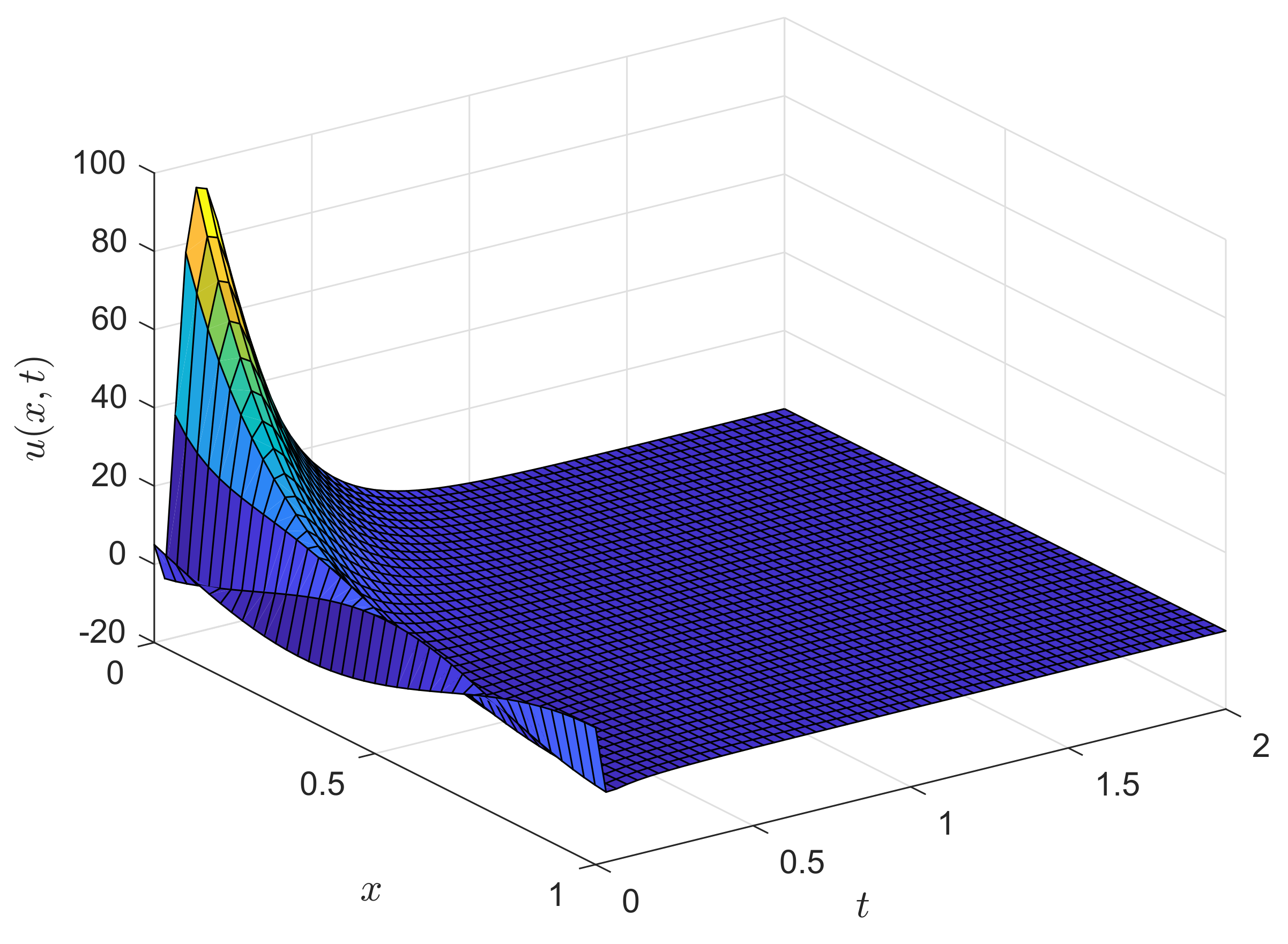
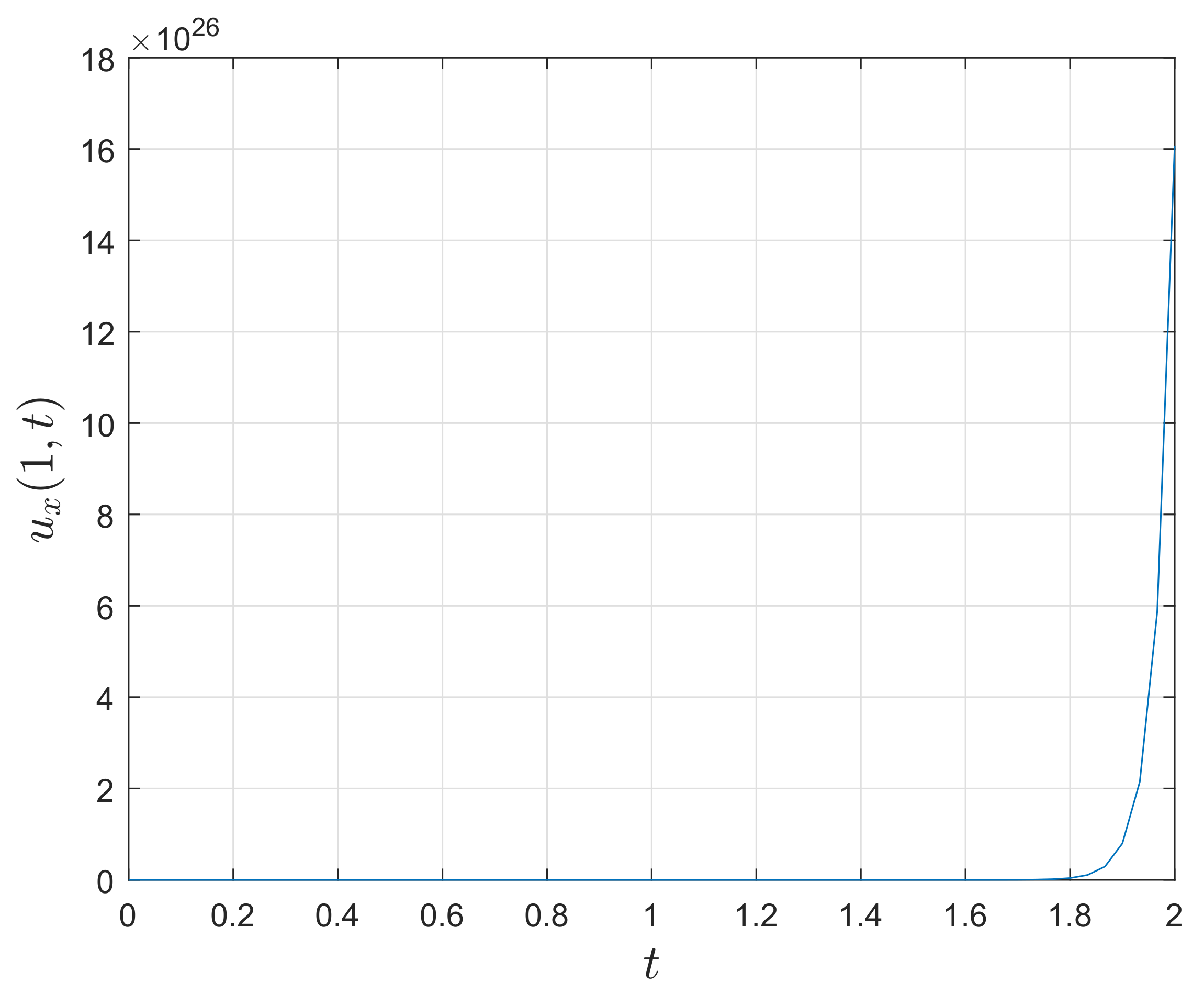
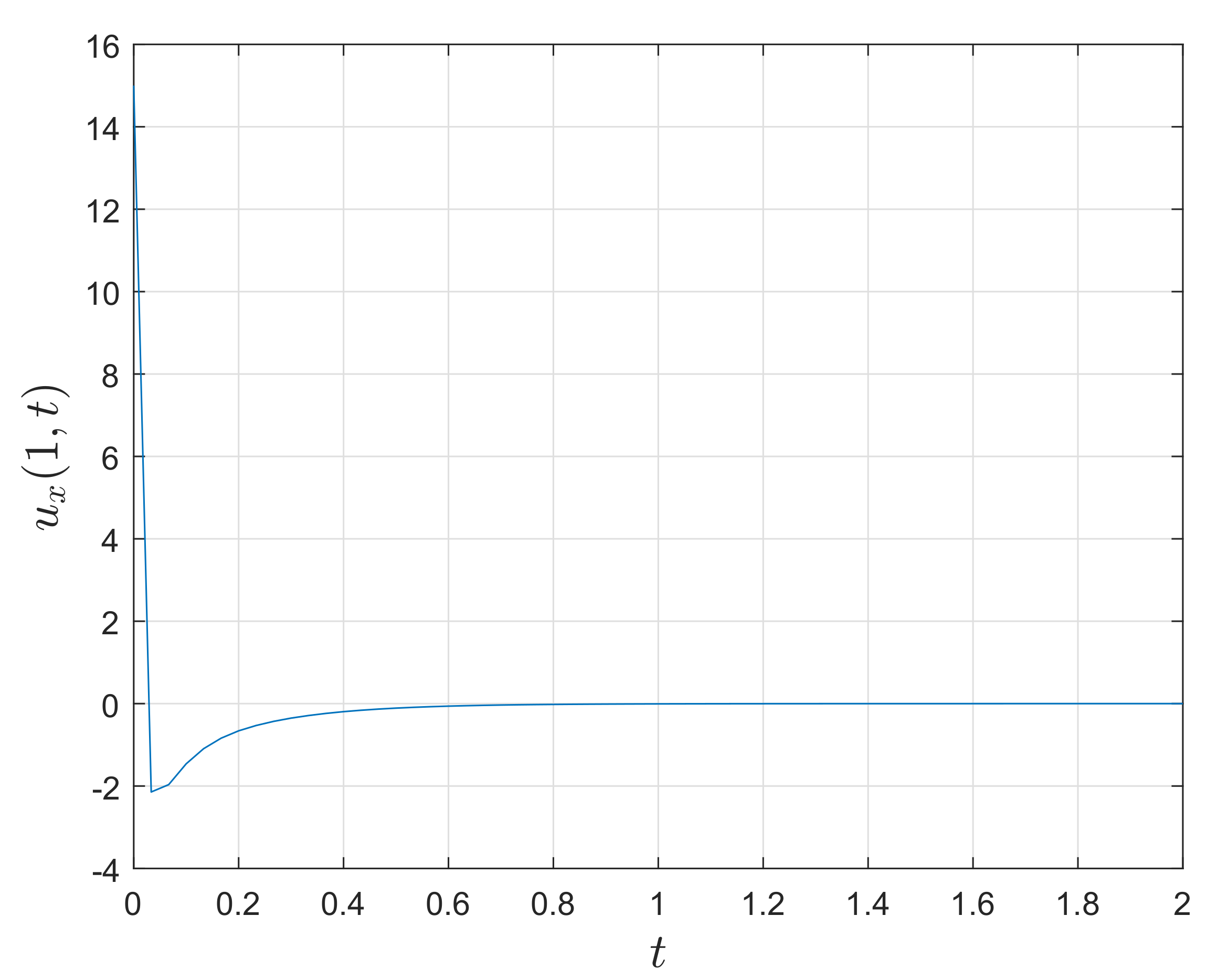
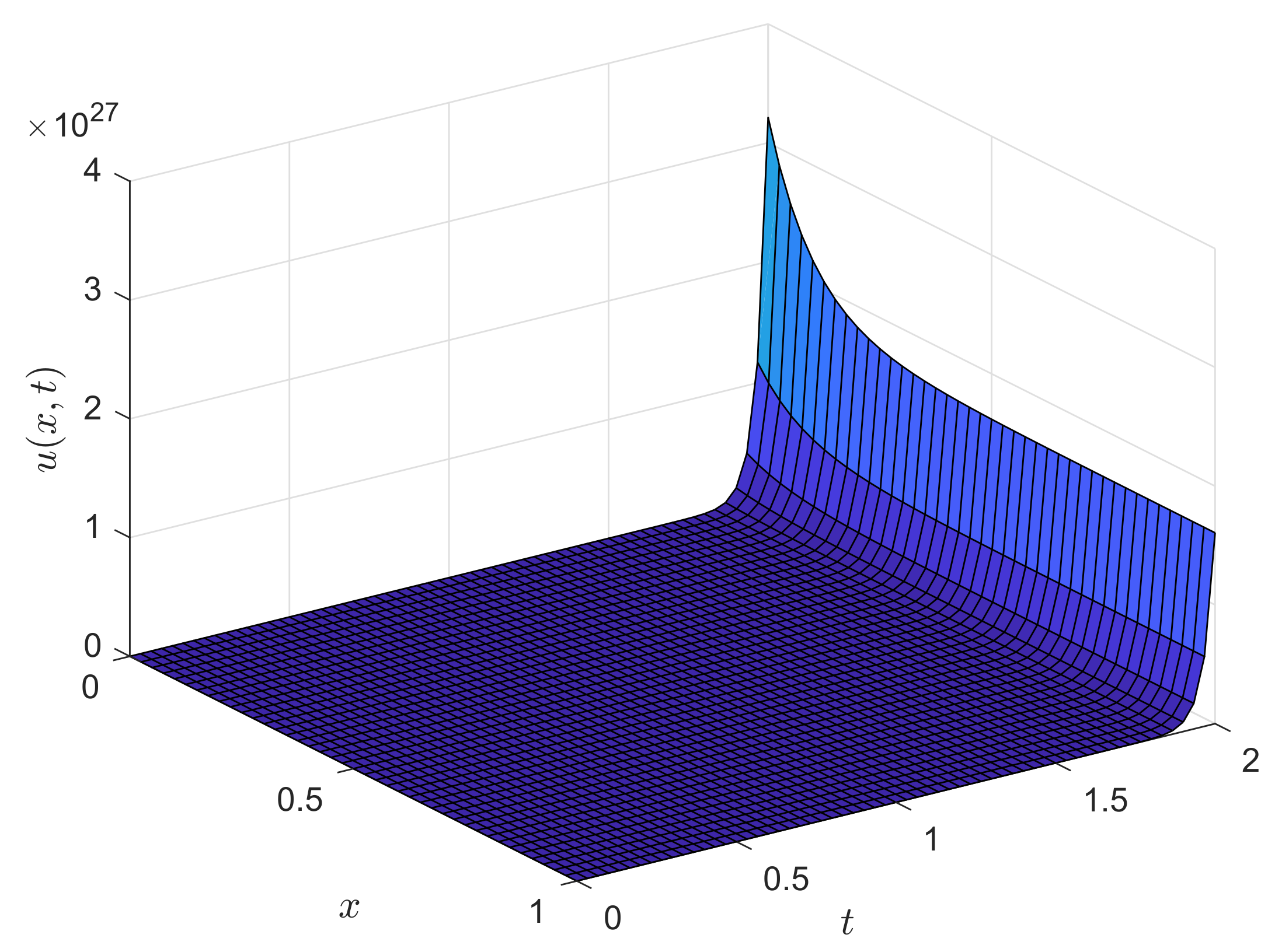
In this section, we exhibit simulation results for both open- and closed-loop dynamics of the PDE system (13)–(15). The aim is to show that the Neumann stabilizing controller (126) applied at the boundary condition (15) achieves boundary control of the R-A-D system. The open-loop dynamic behavior is that for which $\mathcal{U}\left(t\right)=0$. The parameters for the PDE (13), and for which the code was executed, are $\lambda =30$ and $b=10$ with initial condition $u_0\left(x\right)=5\left(1-2sin\left(\frac{3\pi x}{2}\right)\right)$. Figure 1 shows the open-loop dynamic behavior of the R-A-D system from which it can be seen that the system is unstable. From Figure 2, it can be seen that the closed-loop response from the boundary control of the PDE system the controller makes of this PDE system a stable one. Figure 3 shows the open-loop response behavior at the right boundary for $u_x(1,t)=0$. Figure 4 shows the control effort when applying the Neumann stabilizing controller (126) at the right boundary of the R-A-D system in order to implement the closed-loop system. From Figure 4, it can be seen that the control effort is bounded.

10. Conclusions

In this work, a Neumann stabilizing controller to the boundary control of a certain class of reaction-advection-diffusion (R-A-D) system, with constant parameters to the PDE and Neumann boundary conditions, via backstepping approach is designed. The performance of the stabilizing controller is validated via numerical simulation. Simulation results show that the control goal has been achieved. Furthermore, our numerical algorithm based on MATLAB® is provided in order to replicate the simulation results. It should be noticed that our numerical algorithm also has been validated for others problems about boundary control of PDEs but with the restriction that the PDEs must be of parabolic or elliptic type. As future work, from the R-A-D system used here, the approaches proposed in [20,21,22,23] could be explored.

References

1. Haberman, R. Elementary Applied Partial Differential Equations: With Fourier Series and Boundary Value Problems; Prentice Hall: Englewood Cliffs, NJ, USA, 1987. [Google Scholar]
2. Krstic, M.; Kanellakopoulos, I.; Petar, V. Nonlinear and Adaptive Control Design; Wiley: New York, NY, USA, 1995. [Google Scholar]
3. Khalil, H. Nonlinear Systems; Prentice Hall: Englewood Cliffs, NJ, USA, 2002. [Google Scholar]
4. Balogh, A.; Miroslav, K. Infinite Dimensional Backstepping-Style Feedback Transformations for a Heat Equation with an Arbitrary Level of Instability. Eur. J. Control 2002, 8, 165–175. [Google Scholar] [CrossRef]
5. Liu, W. Boundary Feedbak Stabilization of an Unstable Heat Equation. SIAM J. Control Optim. 2003, 42, 1033–1043. [Google Scholar] [CrossRef]
6. Smyshlyaev, A.; Krstic, M. Closed-Form Boundary State Feedbacks for a Class of 1-D Partial Integro-Differential Equations. IEEE Trans. Autom. Control 2004, 49, 2185–2202. [Google Scholar] [CrossRef] [Green Version]
7. Smyshlyaev, A.; Krstic, M. Backstepping Observers for a Class of Parabolic PDEs. Syst. Control Lett. 2005, 54, 613–625. [Google Scholar] [CrossRef]
8. Smyshlyaev, A.; Krstic, M. Output-Feedback Adaptive Control for Parabolic PDEs with Spatially Varying Coefficients. In Proceedings of the 45th IEEE Conference on Decision and Control, San Diego, CA, USA, 13–15 December 2006. [Google Scholar]
9. Smyshlyaev, A.; Krstic, M. Adaptive Boundary Control for Unstable Parabolic PDEs—Part II: Estimation-based Designs. Automatica 2007, 43, 1543–1556. [Google Scholar] [CrossRef]
10. Smyshlyaev, A.; Krstic, M. Adaptive Boundary Control for Unstable Parabolic PDEs—Part III: Output Feedback Examples with Swapping Identifiers. Automatica 2007, 43, 1557–1564. [Google Scholar] [CrossRef]
11. Krstic, M.; Smyshlyaev, A. Adaptive Boundary Control for Unstable Parabolic PDEs—Part I: Lyapunov Design. IEEE Trans. Autom. Control 2008, 53, 1575–1591. [Google Scholar] [CrossRef]
12. Smyshlyaev, A.; Krstic, M. Adaptive Control of Parabolic PDEs; Princeton University Press: Princeton, NJ, USA, 2010. [Google Scholar]
13. Krstic, M.; Smyshlyaev, A. Boundary Control of PDEs: The Backstepping Approach in The Control Handbook, 2nd ed.; Levine, W.S., Ed.; CRC Press: Boca Raton, FL, USA, 2011. [Google Scholar]
14. Krstic, M.; Smyshlyaev, A. Boundary Control for PDEs: A Course on Backstepping Designs; SIAM: Philadelphia, PA, USA, 2008. [Google Scholar]
15. Anfinsen, H.; Aamo, O.M. Adaptive Control of Hyperbolic PDEs; Springer: Cham, Switzerland, 2019. [Google Scholar]
16. Karafyllis, I.; Krstic, M. Input-to-State Stability for PDEs; Springer: Cham, Switzerland, 2019. [Google Scholar]
17. Temam, R. Infinite-Dimensional Dynamical Systems in Mechanics and Physics; Springer: New York, NY, USA, 1998. [Google Scholar]
18. Abramowitz, M.; Stegun, I.A. Handbook of Mathematical Functions: With Formulas, Graphs, and Mathematical Tables; Dover Publications: Mineola, NY, USA, 1965. [Google Scholar]
19. MATLAB R2018a; ©1984-2018; The MathWorks, Inc.: Natick, MA, USA, 2018.
20. Vazquez, R.; Krstic, M. Boundary Control of Coupled Reaction-Advection-Diffusion Systems with Spatially-Varying Coefficients. IEEE Trans. Autom. Control 2016, 62, 2026–2033. [Google Scholar] [CrossRef] [Green Version]
21. Pisano, A.; Baccoli, A.; Orlov, Y.; Usai, E. Boundary control of coupled reaction-advection-diffusion equations having the same diffusivity parameter. IFAC-PapersOnLine 2016, 49, 86–91. [Google Scholar] [CrossRef]
22. Ren, Z.; Xu, C.; Zhou, Z.; Wu, Z.; Chen, T. Boundary stabilization of a class of reaction–advection–diffusion systems via a gradient-based optimization approach. J. Frankl. Inst. 2019, 356, 173–195. [Google Scholar] [CrossRef]
23. Wang, S.; Diagne, M.; Qi, J. Adaptive Control of Reaction-Advection-Diffusion PDEs with Distributed Actuation and Unknown Input Delay. In Proceedings of the American Control Conference (ACC), Denver, CO, USA, 1–3 July 2020. [Google Scholar]
Figure 1. Open-loop response from the solution of the R-A-D PDE.
Mathematics 08 01854 g001
Figure 2. Closed-loop response from the solution to the R-A-D PDE with boundary control.
Mathematics 08 01854 g002
Figure 3. Open-loop behavior at the right hand side boundary from the R-A-D PDE.
Mathematics 08 01854 g003
Figure 4. Closed-loop control effort at the right hand side boundary from the R-A-D PDE.
Mathematics 08 01854 g004
Publisher’s Note: MDPI stays neutral with regard to jurisdictional claims in published maps and institutional affiliations.