Abstract
In the survival data analysis, commonly, it is presumed that all study subjects will eventually have the event of concern. Nonetheless, it tends to be unequivocally expected that a fraction of these subjects will never expose to the event of interest. The cure rate models are usually used to model this type of data. In this paper, we introduced a maximum likelihood estimates analysis for the four-parameter exponentiated Weibull exponential (EWE) distribution in the existence of cured subjects, censored observations, and predictors. Aiming to include the fraction of unsusceptible (cured) individuals in the analysis, a mixture cure model, and two non-mixture cure models—bounded cumulative hazard model, and geometric non-mixture model with EWE distribution—are proposed. The mixture cure model provides a better fit to real data from a Melanoma clinical trial compared to the other two non-mixture cure models.
1. Introduction
In survival analysis, the Weibull distribution is broadly used in cancer research studies [1] since its hazard function is adjustable and it is easy to estimate its parameters. Nevertheless, datasets in medicine studies commonly need more advanced parametric models. Therefore, to accomplish this objective, Weibull distribution has been extended to new classes of parametric distributions, for instance, the exponentiated Weibull [2], the generalized modified Weibull [3], and the exponentiated Weibull exponential distributions [4]. Furthermore, another popular circumstance in the survival data analysis happens, especially in cancer studies, when a portion of individuals is not exposed to the event of concern. For this situation, if the distribution of survival time for susceptible patients is specified, researchers usually prefer cure fraction models to parametric models. Cure fraction models play an important role in the analysis of survival data with long-term survivors and are considered as an extended version of the ordinary survival models. These models have been an object of research since the 1940s. The two main classes of the cure fraction models are mixture and non-mixture cure models. The assumption of the mixture cure model is that the population is divided into two groups, namely unsusceptible (cured) and susceptible (uncured). The mixture cure model was first suggested by Boag [5] and, after three years, Berkson and Gag [6] developed it further. Many researchers have extensively studied the mixture cure model, for instance, Farewell [7], Goldman [8], Kuk and Chen [9], Taylor [10], Maller and Zhou [11], Peng and Dear [12], Zhang and Peng [13] and Patilea and Van Keilegom [14], among others. Chen et al. [15] suggested that the proportional hazard property for the entire population is not validated by the mixture cure model. On the contrary, the non-mixture cure model was suggested to verify this property for all observations, while enabling the direct inference of the predictors of the probability of being cured [16,17]. In their analysis of the previous study on the bounded cumulative hazard model using statistical inference, Tsodikov et al. [18] pointed out that the bounded cumulative hazard model is simple in terms of computations, has a meaningful biological interpretation, and its structure is flexible for the survival function that could provide some technical advantage when designing procedures for maximum likelihood estimation. The literature has suggested various approaches to model the non-mixed cure model, see [19,20,21,22].
Cooner et al. [23] developed a unifying versatile family of cure models using latent activation schemes. They provided the generalization for the bounded cumulative hazard model formula and stated the marginal distribution of as
where is the expectation calculated over , is a survival function of latent event times, denotes the number of colognes cells, and it can have any distribution with finite-mean integer-values, is the respective moment generating function (mgf), and a cure rate defined by . Based on work in [23], further possibilities for the distributions of beyond the Poisson distribution can be assumed, such as the geometric and negative binomial distributions.
When modelling survival data with cured possibility, researchers are concerned about the specification of distribution for the survival times of susceptible subjects, and the effect of independent variables on cure rate and survival times. These two issues are very important in the analysis of lifetime data. Cure fraction models can be applied for the analysis of the lifetime data in the existence of cured subjects, and factors affecting the probability of being cured. An appropriate distribution for survival times needs to be specified. Disregarding this specification may result in unreliable parameter estimations. For survival data with cured possibility, and the ability to identify a suitable distribution for survival time, cure fraction models are preferable to classical survival models.
The literature presents detailed research on cure fraction models regarding the choice of the best model that fits the data and influences of covariates on the probability of being cured and survival times of susceptible individuals. For more details on the effect of covariates on the response variable, we refer the reader to [24,25,26]. Several works comparing the cure models’ performance regarding the predictors’ effects on the cure fraction and survival times were done under the mixture cure model and the bounded cumulative hazard model. However, a few other formulations of non-mixture cure models have been employed. Therefore, in the present study, we propose a cure fraction model with more flexible distribution for survival times and a geometric distribution for the latent variable.
In this article, we compare the performance of the mixture cure model, the bounded cumulative hazard model, and the geometric non-mixture cure model based on exponentiated Weibull exponential [4], which is flexible to accommodate different forms of the failure rate function. For illustration, we use a melanoma dataset E1684, which is available in R package smcure [27], considering the existence of the cure rate, censored observations, and predictors. Statistical analysis of this data is performed under the maximum likelihood estimation technique.
This study aims to specify uncured melanoma patients’ survival times, to discuss the effects of predictors on cure rate and survival times simultaneously, and to contribute to this growing area of research by exploring the usefulness of the EWE distribution for the analysis of right-censored data.
The rest of the paper is outlined as follows. In Section 2, we describe a melanoma dataset. Section 3 introduces the mixture cure model, the bounded cumulative hazard model, and the geometric non-mixture cure models. Section 4 presents the EWE distribution and particular cases related to it. The log-likelihood functions of the three proposed cure models are derived in Section 5. The model choice is explained in Section 6. In Section 7, we report on the results obtained from the maximum likelihood estimation approach considering all cure models of interest fitted over the melanoma data. We present a discussion in Section 8.
2. Melanoma Data
Melanoma is a dangerous form of skin cancer that starts in cells called melanocytes cells. The incidence of melanoma rises at a rate beyond all solid tumors. In the United States, the overall incidence of melanoma is estimated at 22.7 per 100,000 persons [28]. According to [29], 100,350 people are estimated as new cases, and 6850 people are expected to die due to melanoma in 2020. Nonetheless, in recent years, the chances of cure for patients with melanoma have increased due to the earlier diagnosis and development of treatment and surgical techniques. It is worth mentioning that recent research indicates that applying oleocanthal obtained from olive oil to human malignant melanomas found that it had anti-cancer activity, suggesting that olive oil potentially helps protect against skin cancer [30]. For more details about the olive oil industry, see [31]. Even though the majority of melanoma patients are cured by their initial therapy, it is unattainable to differentiate them from uncured patients. Therefore, it is of great importance to precisely estimate the probability of being cured to plan further treatment to improve the survival of uncured melanoma patients.
In this study, we consider E1684 phase III melanoma data which is obtained from a clinical trial conducted by the Eastern Cooperative Oncology Group (ECOG). This trial was a two-arm clinical trial: high-dose interferon alpha −2b (IFNα − 2b) versus control (Observe). A total of 284 patients participated in this trial, of whom 113 (40%) were female. Of the total number of patients, 144 (51%) were exposed to the IFN treatment, and we found that 196 (69%) of patients experienced cancer relapse. The remaining individuals were right-censored. For more details about these data, see Kirkwood et al. [32].
Figure 1a displays the overall survival curve of the melanoma data, which was obtained based on the Kaplan–Meier technique; the existence of a “plateau” near to 0.3 in the curve suggests that a cure fraction model is appropriate for the analysis of these data. The graph in Figure 1b shows survival curves for the two types of treatment where steady plateaus can be seen at the right tail for each curve, and this also confirms the efficacy of the cure model approach.
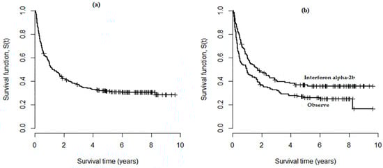
Figure 1.
(a) Overall survival curve obtained by Kaplan–Meier approach for the e1684 data; (b) Survival curves for the two types of treatments.
The literature shows different studies related to the analysis of the melanoma data E1686. For example, in the works of [15,23], it was presumed that the predictors only influence the cure fraction, while Kutal and Qian [22] did not consider the covariates in their analysis. Here, we link the covariates with both cure rate and survival times to discuss their effect on the probability of being cured and the survival time of susceptible patients.
3. Cur Models
In the literature, there are two main types of cure models that have been suggested to fit lifetime data in medical studies, namely, mixture cure and non-mixture cure models. These models can be applied for the analysis of real-life data in fields other than the medical field, for instance, in economics, reliability, criminology, sociology education, and marketing, among others. The modelling approach varies based on the researcher’s event of interest; the common idea is to observe time until the event, but for some subjects, the event will never occur.
In this section, we introduce the mixture cure model and two different formulations of the non-mixture cure model.
3.1. Mixture Cure Model
A mixture cure model (MCM) is a common approach for modelling data with long-term survivors. The advantage of the MCM is that it enables covariates to have different effects on patients who are cured and on the survival times of susceptible patients. On the other hand, this model cannot verify the property of proportional hazard functions. Besides, the MCM does not appear to have a biological interpretation meaning, especially in the cancer recurrence studies.
Let denote the event’s time occurrence and let be a probability of being cured. Furthermore, for susceptible subjects, assume that and are survival and density functions, respectively. Thus, the entire population survival function is
and the corresponding probability density function is
For , different parametric distributions can be chosen, for instance, exponential, Weibull and Fréchet.
Suppose we have a random sample of size , and we observe the pair in which represents the censoring indicator variable that takes the values zero and one for censored and uncensored observations, respectively, and Considering MCM model (2), the likelihood function is
3.2. Bounded Cumulative Hazard Model (BCH)
Suggested by Yakovlev et al. [33], the BCH model provides a different method to model a cure fraction. The mathematical definition of the BCH model shows that this model has a bounded cumulative hazard function, and its survival function takes the form
where is the cumulative distribution function. For the BCH model (4), the likelihood function is
in which is the hazard function.
3.3. Geometric Non-Mixture Cure Model
Following Cooner et al. [23], we assume that after the patient is exposed to genetic spoilage, his body produced mutated cells/tissues before the activation of the immune system. If the probability of producing each new mutated cell is an efficient immune system able to devastate the last mutated cell to pause the process of mutation, then has a geometric distribution with probability mass function and mean . The corresponding mgf, may be derived as follows
Let be the independently and identically distributed promotion times of mutated cells remaining in the body and ; then, from Equations (1) and (6), we have
which is the survival function of the entire population. In this case, the cure fraction can be defined as
In what follows, we refer to the model in (7) as a geometric non-mixture cure model (GNMCM) and we have . Considering the GNMCM, the probability density function for the lifetime is given by
and the respective risk function takes the form
Moreover, the likelihood function for GNMCM is
The GNMCM is appealing in many respects. First, it has a biologically meaningful interpretation; second, its hazard function has an interesting structure. In contrast to the BCH model, the hazard ratio is not constant over time.
4. Exponentiated Weibull Exponential Distribution (EWE)
Let us assume the EWE as a distribution of the susceptible subjects’ survival time. This distribution has the following density function
where represents two shape parameters and are the two scale parameters. Elgarhy et al. [4] proposed this distribution, which is adequate for accommodating different hazard failure function shapes, including those that are bathtub-shaped. The survival function of EWE distribution may be written as
The EWE distribution is denoted by and its risk function takes the form
Equation (10) contains different sub-distributions of EWE distribution Elgarhy et al. [4]. These distributions are given as follows:
- Exponentiated exponential exponential (EEE): when , the Equation (10) reduces to the probability density function of an EEE, which is
- Exponentiated Rayleigh exponential (ERE): when we substitute in the Equation (10), we havewhich expresses the density function of an ERE distribution;
- Weibull exponential (WE): when , the Equation (10) becomes the probability density function of the WE distribution, which isOguntude et al. [34] discuss the statistical properties of the WE distribution;
- Exponential exponential (EE): if in the Equation (10), we havewhich is the probability function of an EE distribution;
- Rayleigh Exponential (RE): this is special case of the EWE distribution when . Its density function is given by
5. The Log-Likelihood Functions
Let and assume the MCM (2), then the log-likelihood function for is
The log-likelihood function for under the BCH (4) can be expressed as
Moreover, regarding the GNMCM model (6), the log-likelihood function for may be written as
Furthermore, for these three cure models, we assume that the probability of being cured is “” and the shape parameter “” could be linked to a vector of covariates by substituting “”and “” in the expressions (11)–(13) by
and
where and are two sets of unknown coefficients.
6. Model Choice
The comparison between MCM, BCH model and GNMCM based on different distributions was evelauated by applying the Akaike Information Criteria (AIC) proposed by [35], the Bayesian Information Criteria (BIC) introduced by [36], and Hannan-Quinn Information Criteria (HQIC) suggested by [37]. A smaller value of information criteria indicates a preferable model fit. The AIC, BIC and HQIC are defined as follows
where is the likelihood function, represents the number of free parameters in the model, and is the number of observations.
7. Results
In Table 1, Table 2 and Table 3, we have the maximum likelihood estimates, standard errors, and information criterion values for AIC, BIC, and HQIC obtained by MCM, the BCH model, and GNMCM based on the probability distributions of interest considering the melanoma data and not including covariates, respectively. From Table 1, it is apparent that the smallest values of selection criteria are provided by EWE distribution, which indicates that the MCM based on this distribution is the preferable model compared with EEE, ERE, WE, and RE distributions. Considering Table 2, it is clear that the BCH model with EWE distribution is the best in comparison with the other parametric distributions. Using the results in Table 3, we note that the GNMCM based on EWE distribution also provides a better fit to the data compared with the other particular cases of EWE distributions. Assuming EWE distribution, and comparing MCM, the BCH model, and GNMCM, we observe similar results, which indicates that the three cure models fit the data equally. Therefore, the GNMCM is a good candidate to be considered. However, the MCM illustrates slightly better results, which indicates that this model provides a better fit to the data compared with the BCH model and GNMCM. These conclusions are demonstrated in Figure 2 and Figure 3.

Table 1.
Results of maximum likelihood estimates, considering the mixture cure model (MCM) for e1684 data without covariates.
Table 2.
Results of maximum likelihood estimates, considering the bounded cumulative hazard (BCH) model for e1684 data without covariates.
Table 3.
Results of maximum likelihood estimates, considering the geometric non-mixture cure model (GNMCM) for e1684 data without covariates.
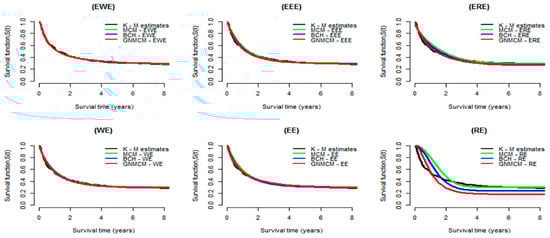
Figure 2.
Estimated survival curves for the melanoma data obtained from the MCM, BCH and GNMCM based on the EWE distribution and its special cases. For comparison purpose, curves of Kaplan–Meier estimates are displayed in all plots.
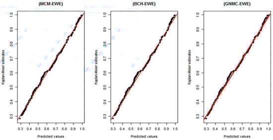
Figure 3.
Plots of the Kaplan–Meier estimates for the survival functions versus the respective estimated survival values provided by MCM, BCH and GNMCM based on the EWE distribution. An ideal consent between the predicted survival values and Kaplan–Meier estimates is represented by the diagonal straight lines.
Figure 2 illustrates the Kaplan–Meier curves with predicted survival curves (results from Table 1, Table 2 and Table 3). From this figure, we observe that the estimated curves obtained by MCM, BCH model and GNMCM based on the EWE distribution (top left panel) are very close to the curves of Kaplan–Meier, compared to all other distributions, suggesting that the EWE distribution provides a better fit to the data. Moreover, WE, EE, and ER distributions, after we exponentiated them, became EWE, EEE, and ERE, respectively. They significantly improve the estimation of the survival function; this can be seen clearly in the case of RE and ERE distributions.
Plots of survival curves obtained by the Kaplan–Meier approach versus respective predicted survival values obtained by MCM, BCH and GNMCM based on EWE distribution are depicted in Figure 3. There is no significant difference between the graphs in the three panels, which illustrates that these three cure models based on EWE distribution equally fit the data.
To discuss the effect of the predictors on the probability of cure and survival function shape, three covariates, sex (zero for male, 1 for female), treatment (zero for Observe group, 1 for IFN treatment group) and age, are linked to the cure fraction “” and the shape parameter “” using the expressions (14) and (15). Therefore, we have
and
where denotes the patient gender, for the treatment type and is the age of the patient. Table 4 presents the maximum likelihood estimates, 95% confidence intervals, and information criterion values obtained by the MCM, BCH, and GNMCM based on the EWE distribution for the melanoma data with covariates. From this table, we note that the values of each one of three selection criteria are quite similar, meaning that these models likely fit the data equally. However, the MCM model provides a better fit to the data compared to the BCH model and GNMCM. Moreover, the 95% confidence intervals for , in the three cure models, do not include the value of zero, which indicates that the IFN treatment has a significant influence on the cure rate. The predictors, namely, sex and age, do not significantly affect the cure rate and the shape of the survival function.
Table 4.
Maximum likelihood estimate results, obtained by MCM, BCH and GNMC models with the EWE distribution for the melanoma data, and the covariates are linked all to the cure fraction parameter “” and the parameter of shape “a”.
Since the MCM based on EWE distribution shows a better fit for the melanoma data (with and without covariates) compared with the BCH model and GNMCM, we focus on the MCM model to analyze these data further. Figure 4a presents the predicted population survival curves provided by MCM with EWE distribution, where the respective estimated susceptible survival functions are illustrated in Figure 4b (values of Table 4). There is a significant dissimilarity in the population survival functions between treatment groups. Similar conclusions could be drawn if we consider the two non-mixture cure models (BCH and GNMCM).
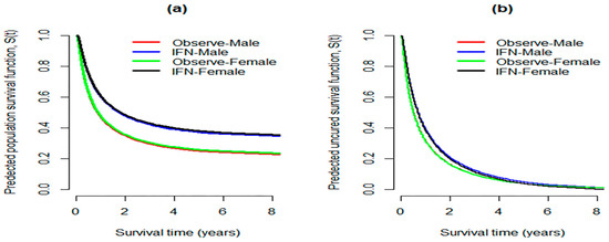
Figure 4.
(a) Predicted population survival functions between groups calculated at median value of AGE; (b) predicted survival function of the uncured patients between groups, considering e1684 data.
Figure 5 illustrates the fitted population risk functions (Figure 5a), and the estimated susceptible hazard functions (Figure 5b) obtained by the MCM based on EWE distribution (results of Table 4). From this figure, we notice that, during the first two years after treatment, the predicted population risk functions reveal that the hazard of cancer relapse diminishes sharply until a value of about 0.11, and then gradually decreases until the end of the study. The danger of cancer relapse for susceptible patients is very high immediately after the treatment, declines rapidly until a value of around 0.5, and almost remains constant around this value till the end of the follow-up time.
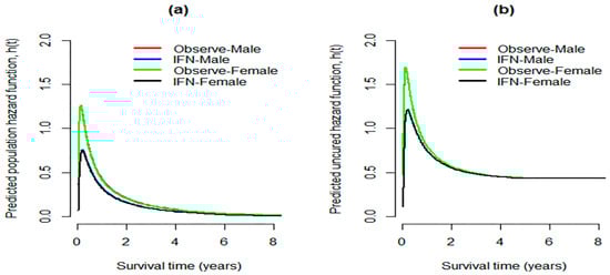
Figure 5.
(a) Predicted population risk functions considering MCM model with EWE distribution; (b) respective susceptible hazard functions.
8. Discussion
The present study aims to specify the distribution of the survival times of susceptible melanoma E1684 patients and to investigate the influence of covariates on cure rates and survival times. To achieve these goals, we propose three cure fraction models—MCM, BCH model, and GNMCM—based on EWE distribution for the analysis of the melanoma data.
Cure fraction models are useful for estimating the probability of being cured. Moreover, they can be reduced to classical survival models when there are no cure subjects in the population under study. The important issues associated with cure models are identifiability of the cure rate, the distribution of survival time of susceptible subjects, and the length of follow-up time. Discussion of these issues is beyond the scope of this study.
The Kaplan–Meier curve is usually used to identify the presence of cure subjects. If the right tail of the curve is long and steady (shows a plateau level), then there would be evidence of the existence of cure subjects. The graph in Figure 1 provides evidence that a cure fraction exists. Therefore, we compared the performance of the MCM, BCH, and GNMCM considering different susceptible distributions for the e1684 data. We observe that the three cure models provide similar results. However, the MCM model based on EWE distribution is found to be the best model to fit the given data, suggesting that the distribution of survival times of uncured melanoma patients followed from EWE distribution in the best way. Moreover, the treatment has a significant influence on the cure fraction within all the models, indicating that the Interferon alpha − 2b improves the rate of cure, and these results are in agreement with the findings of [21,38]. Besides this, the results of this study are also consistent with those of [39], who concluded that the melanoma recurrence probability is lower for the treatment group compared to the observed group. It is worth mentioning that the other covariates (age and sex) have no significant effect on the probability of being cured and the shape of the survival function; this may be due to the similarity between the immune systems of men and women in their response to melanoma cancer and IFN treatment.
In conclusion, in the analysis of melanoma patients’ data, we found that the EWE distribution is the best distribution for the survival time of susceptible patients compared with EEE, ERE, EE, WE, and RE distributions. Moreover, the interferon alpha − 2b significantly ameliorates the portion of immune patients, while the predictors, age, and sex did not show a considerable influence on cure fraction. In addition to that, the results of this study reveal that the GNMCM can be considered as a good candidate to model these data.
The study undertaken has highlighted a topic on which further research would be beneficial, and this relates to an analysis of the e1684 data. It might be possible to use alternative generalized distributions under the Bayesian inference techniques, because the experience of an oncologist on an anticipated fraction of patients who are cured can be included in a prior distribution of the parameter of the cure rate, , resulting in more accurate inferences.
Author Contributions
Conceptualization: M.E.A.M.E.O., M.R.A.B., M.B.A. and M.S.M.; Methodology: M.E.A.M.E.O., M.R.A.B., M.B.A. and M.S.M.; Software: M.E.A.M.E.O., M.R.A.B., M.B.A. and M.S.M.; Writing—original draft: M.E.A.M.E.O., M.R.A.B., M.B.A. and M.S.M. All authors have read and agreed to the published version of the manuscript.
Funding
This research received no external funding.
Acknowledgments
The authors are grateful to thank the anonymous referee for their careful review and insightful comments that have led to significant improvement of this article.
Conflicts of Interest
The authors declare no conflict of interest.
References
- Bradburn, M.J.; Clark, T.G.; Love, S.B.; Altman, D.G. Survival analysis Part III: Multivariate data analysis —Choosing a model and assessing its adequacy and fit. Br. J. Cancer 2003, 89, 605–611. [Google Scholar] [CrossRef]
- Mudholkar, G.S.; Srivastava, D.K. Exponentiated Weibull family for analyzing bathtub failure-rate data. IEEE Trans. Reliab. 1993, 42, 299–302. [Google Scholar] [CrossRef]
- Carrasco, J.M.F.; Ortega, E.M.M.; Cordeiro, G.M. A generalized modified Weibull distribution for lifetime modeling. Comput. Stat. Data Anal. 2008, 53, 450–462. [Google Scholar] [CrossRef]
- Elgarhy, M.; Shakil, M.; Kibria, B.M.G. Exponentiated Weibull-exponential distribution with applications. AAM Int. J. 2017, 12, 710–725. [Google Scholar]
- Boag, J.W. Maximum likelihood estimates of the proportion of patients cured by cancer therapy. J. R. Stat. Soc. Ser. B Methodol. 1949, 11, 15–53. [Google Scholar] [CrossRef]
- Berkson, J.; Gage, R.P. Survival curve for cancer patients following treatment. J. Am. Stat. Assoc. 1952, 47, 501–515. [Google Scholar] [CrossRef]
- Farewell, V.T. The use of mixture models for the analysis of survival data with long-term survivors. Biometrics 1982, 38, 1041–1046. [Google Scholar] [CrossRef]
- Goldman, A.I. Survivorship analysis when cure is a possibility: A Monte Carlo study. Stat. Med. 1984, 3, 153–163. [Google Scholar] [CrossRef]
- Kuk, A.Y.C.; Chen, C.H. A mixture model combining logistic regression with proportional hazards regression. Biometrika 1992, 79, 531–541. [Google Scholar] [CrossRef]
- Taylor, J.M.G. Semi-parametric estimation in failure time mixture models. Biometrics 1995, 51, 899–907. [Google Scholar] [CrossRef]
- Maller, R.A.; Zhou, X. Survival Analysis with Long-Term Survivors; Wiley: New York, NY, USA, 1996; ISBN 0-471-96201-5. [Google Scholar]
- Peng, Y.; Dear, K.B.G. A nonparametric mixture model for cure rate estimation. Biometrics 2000, 56, 237–243. [Google Scholar] [CrossRef] [PubMed]
- Zhang, J.; Peng, Y. Accelerated hazards mixture cure model. Lifetime Data Anal. 2009, 15, 455–467. [Google Scholar] [CrossRef]
- Patilea, V.; Van Keilegom, I. A general approach for cure models in survival analysis. arXiv 2017, arXiv:170103769. [Google Scholar] [CrossRef]
- Chen, M.-H.; Ibrahim, J.G.; Sinha, D. A new bayesian model for survival data with a surviving fraction. J. Am. Stat. Assoc. 1999, 94, 909–919. [Google Scholar] [CrossRef]
- Klebanov, L.B.; Rachev, S.T.; Yakovlev, A.Y. A stochastic model of radiation carcinogenesis: Latent time distributions and their properties. Math. Biosci. 1993, 113, 51–75. [Google Scholar] [CrossRef]
- Tsodikov, A. A proportional hazards model taking account of long-term survivors. Biometrics 1998, 54, 1508–1516. [Google Scholar] [CrossRef]
- Tsodikov, A.D.; Ibrahim, J.G.; Yakovlev, A.Y. Estimating cure rates from survival data: An alternative to two-component mixture models. J. Am. Stat. Assoc. 2003, 98, 1063–1078. [Google Scholar] [CrossRef]
- Uddin, M.T.; Sen, A.; Noor, M.S.; Islam, M.N.; Chowdhury, Z.I. An analytical approach on non-parametric estimation of cure rate based on uncensored data. J. Appl. Sci. 2006, 6, 1258–1264. [Google Scholar] [CrossRef]
- Liu, H.; Shen, Y. A semiparametric regression cure model for interval-censored data. J. Am. Stat. Assoc. 2009, 104, 1168–1178. [Google Scholar] [CrossRef]
- Bremhorst, V.; Lambert, P. Flexible estimation in cure survival models using Bayesian P-splines. Comput. Stat. Data Anal. 2016, 93, 270–284. [Google Scholar] [CrossRef][Green Version]
- Kutal, D.H.; Qian, L. A non-mixture cure model for right-censored data with Fréchet distribution. Stats 2018, 1, 176–188. [Google Scholar] [CrossRef]
- Cooner, F.; Banerjee, S.; Carlin, B.P.; Sinha, D. Flexible cure rate modeling under latent activation schemes. J. Am. Stat. Assoc. 2007, 102, 560–572. [Google Scholar] [CrossRef]
- Abu Bakar, M.R.; Daud, I.; Ibrahim, N.A.; Rahmatina, D. Estimating a logistic Weibull mixture models with long–term survivors. J. Teknol. 2006, 45, 57–66. [Google Scholar] [CrossRef]
- Swain, P.K.; Grover, G.; Goel, K. Mixture and non-mixture cure fraction models based on generalized gompertz distribution under bayesian approach. Tatra Mt. Math. Publ. 2016, 66, 121–135. [Google Scholar] [CrossRef]
- Caruso, G.; Colantonio, E.; Gattone, S.A. Relationships between Renewable energy consumption, social factors, and health: A panel vector auto regression analysis of a cluster of 12 EU countries. Sustainability 2020, 12, 2915. [Google Scholar] [CrossRef]
- Cai, C.; Zou, Y.; Peng, Y.; Zhang, J. smcure: An R-package for estimating semiparametric mixture cure models. Comput. Methods Programs Biomed. 2012, 108, 1255–1260. [Google Scholar] [CrossRef]
- Centers for Disease Control and Prevention. Available online: https://gis.cdc.gov/Cancer/USCS/DataViz.html (accessed on 21 September 2020).
- American Cancer Society. Available online: https://www.cancer.org/content/dam/cancer-org/research/cancer-facts-and-statistics/annual-cancer-facts-and-figures/2020/cancer-facts-and-figures-2020.pdf (accessed on 21 September 2020).
- Fogli, S.; Arena, C.; Carpi, S.; Polini, B.; Bertini, S.; Digiacomo, M.; Gado, F.; Saba, A.; Saccomanni, G.; Breschi, M.C.; et al. Cytotoxic activity of oleocanthal isolated from virgin olive oil on human melanoma cells. Nutr. Cancer 2016, 68, 873–877. [Google Scholar] [CrossRef]
- D’Adamo, I.; Falcone, P.M.; Gastaldi, M.; Morone, P.; Adamo, D. A social analysis of the olive oil sector: The role of family business. Resources 2019, 8, 151. [Google Scholar] [CrossRef]
- Kirkwood, J.M.; Strawderman, M.H.; Ernstoff, M.S.; Smith, T.J.; Borden, E.C.; Blum, R.H. Interferon alfa-2b adjuvant therapy of high-risk resected cutaneous melanoma: The Eastern Cooperative Oncology Group Trial EST 1684. J. Clin. Oncol. 1996, 14, 7–17. [Google Scholar] [CrossRef] [PubMed]
- Yakovlev, A.; Tsodikov, A. Stochastic Models of Tumor Latency and Their Biostatistical Applications; Asselain, B., Ed.; Mathematical Biology and Medicine; World Scientific Publishing: Singapore, 1996; Volume 1. [Google Scholar]
- Oguntunde, P.E.; Balogun, O.S.; Okagbue, H.I.; Bishop, S.A. The Weibull-exponential distribution: Its properties and applications. J. Appl. Sci. 2015, 15, 1305–1311. [Google Scholar] [CrossRef]
- Akaike, H. A new look at the statistical model identification. IEEE Trans. Autom. Control 1974, 19, 716–723. [Google Scholar] [CrossRef]
- Schwarz, G. Estimating the dimensions of a model. Ann. Stat. 1978, 6, 461–464. [Google Scholar] [CrossRef]
- Hannan, E.J.; Quinn, B.G. The determination of the order of an autoregression. J. R. Stat. Soc. Ser. B Methodol. 1979, 41, 190–195. [Google Scholar] [CrossRef]
- Lázaro, E.; Armero, C.; Gómez-Rubio, V. Approximate Bayesian inference for mixture cure models. TEST 2019, 29, 750–767. [Google Scholar] [CrossRef]
- Musta, E.; Patilea, V.; Van Keilegom, I. A presmoothing approach for estimation in mixture cure models. arXiv 2020, arXiv:200805338. [Google Scholar]
Publisher’s Note: MDPI stays neutral with regard to jurisdictional claims in published maps and institutional affiliations. |
© 2020 by the authors. Licensee MDPI, Basel, Switzerland. This article is an open access article distributed under the terms and conditions of the Creative Commons Attribution (CC BY) license (http://creativecommons.org/licenses/by/4.0/).