Article

Modeling and Solving a Latin American University Course Timetabling Problem Instance

by
Oscar Chávez-Bosquez
,
José Hernández-Torruco
*,
Betania Hernández-Ocaña
* and
Juana Canul-Reich
División Académica de Ciencias y Tecnologías de la Información, Universidad Juárez Autónoma de Tabasco, Cunduacán, Tabasco 86690, Mexico
*
Authors to whom correspondence should be addressed.
Mathematics 2020, 8(10), 1833; https://doi.org/10.3390/math8101833
Submission received: 19 September 2020 / Revised: 8 October 2020 / Accepted: 13 October 2020 / Published: 19 October 2020
(This article belongs to the Section Mathematics and Computer Science)

Abstract

:
Timetabling problem is a complex task that is performed by a number of institutions worldwide, which has been usually addressed as an optimization problem where every approach considers the particular constraints of each institution under consideration. In this paper, we describe, model, and propose a solution to the timetabling problem at the División Académica de Ciencias y Tecnologías de la Información of the Universidad Juárez Autónoma de Tabasco (UJAT), México. We modeled the specific constraints of this problem instance using the Object Constraint Language (OCL) of the Unified Modeling Language (UML), and we validated the model while using the state-of-the-art tool USE: UML-based Specification Environment. The solution strategy tackles the problem in two stages: (1) ACA: academic assignments, i.e., assign lectures to professors and (2) TTP: the timetabling process. We developed a Tabu Search customization named Tabu Search with Probabilistic Aspiration Criterion (TS-PAC) in order to solve the timetabling problem, and we developed a software prototype to test our proposal. Two feasible timetables for two different semesters were obtained according to the modeled constraints.

1. Introduction

Resource allocation is a widespread problem that is faced day by day, from organizing cashiers per shift in a supermarket to the tasking of air assets in an airport. In the academic context, a remarkable problem is the timetabling process, since it is a procedure that a large number of education institutions must perform at least once a year.
Timetabling is an NP-Complete problem [1], so there is no deterministic algorithm that finds an optimal solution in a reasonable time. However, it is possible to use alternative strategies in order to obtain acceptable solutions in a reasonable time. In general, these problems represent a challenge in Computer science, so there is a significant interest in finding efficient methods to solve these problems while using the least amount of resources, i.e., time and computational cost, while providing solutions that are close to the global optimum.
There are different variants of the timetabling problem in the literature, generally differing on the type of institution and its related constraints. Specifically, in this paper, we solve a representative case of the University Course Timetabling problem (UCTP) at the División Académica deCiencias y Tecnologías de la Información (DACyTI), one of 13 divisions of the Universidad Juárez Autónoma de Tabasco (UJAT), México. This timetabling problem instance can be seen as a representative of Latin American universities. However, our institution’s specific problem considers different constraints than other cases [2,3,4], so there is no similar solution in the literature when considering the particular constraints of the timetabling problem at the DACyTI.

2. Preliminaries

2.1. University Course Timetabling Problem

Timetabling is a common and recurring problem that has been extensively analyzed and represented, from the first models presented [5] to the more recently proposed ones [6]. Solution approaches include a full spectrum of strategies, such as mathematical optimization and heuristic algorithms. Either way, each strategy of a solution is raised from a different perspective, particular to the institution at issue, but all agree that the problem modeling is a critical part of creating any solution.
The general case of the timetabling problem, called school timetabling, can be defined as [7]:
  • m classes c 1 , , c m .
  • n teachers t 1 , , t n .
  • p periods of time 1 , , p .
  • a non-negative integer matrix R m * n , called Requirements matrix, where r i j is the number of lectures given by teacher t j to class c i .
The problem consists of assigning lectures to periods of time, such that no teacher or class is involved in more than one lecture at a time. The mathematical formulation is:
Find x i j k ( i = 1 , , m ; j = 1 , , n ; k = 1 , , p ) subject to:
k = 1 p x i j k = r i j ( i = 1 , , m ; j = 1 , , n )
j = 1 n x i j k 1 ( i = 1 , , m ; k = 1 , , p )
i = 1 m x i j k 1 ( j = 1 , , n ; k = 1 , , p )
where x i j k = 1 if class c i and techer t j meet at period of time k, and x i j k = 0 otherwise.
These constraints compose the basic search problem, and any valid timetable represents the solution. However, this basic version of the problem does not consider courses sharing students or the teachers’ course preferences, just to mention some examples of constraints found in most universities.
The university course timetabling problem (UCTP) consists of scheduling a set of lectures for each course within a given number of classrooms and time periods [8] With the particularity that courses might have students in common, unlike school timetabling [9]. Finding a manual solution to the problem typically requires a considerable amount of time, in addition to the validation of an expert, since there may be specific constraints to be considered. These constraints can be of two types  [10]:
  • Hard constraints: mandatory conditions, the violation of any of them implies a non-feasible timetable.
  • Soft constraints: desirable conditions denoting user preferences; the violation of any of them affects the quality of a timetable.
The UCTP can be defined as [7]:
  • q courses K 1 , , K q .
  • Each K course consists of k i lectures.
  • There are r curricula S 1 , , S r , wich are groups of courses that have common students. Thus, courses in S l must be scheduled all at diferent times.
  • A maximum number of lectures l k that can be scheduled at period k (that is, the number of rooms available at period k).
  • A p number of periods of time 1 , , P .
In this case, we want to maximize the desirability of having a lecture of course K i at period of time k. The formal representation is:
Find y i k ( i = 1 , , q ; k = 1 , , p ) subject to:
k = 1 p y i k = k i ( i = 1 , , q )
i = 1 q y i k l k ( k = 1 , , p )
i S i y i k 1 ( l = 1 , , r ; k = 1 , , p )
y i k 0 , 1 ( i = 1 , , q ; k = 1 , , p )
where y i k = 1 if a lecture of course K i is scheduled at period k, and y i k = 0 otherwise.
Objective function (8) is included in the problem definition in order to denote d i k , which is the desirability of assign a lecture of course K i at period k.
Max . i = 1 q k = 1 p d i k y i k
This model can be considered to be a general formulation for the university course timetabling problem. Our institution has many other particular policies that must be considered when generating the timetable. In the following section, we formulate these specific constraints.
Additionally, the typical approach for UCTP includes two stages: (1) to create a feasible solution and (2) to minimize the number of soft constraints violations in the feasible solution [11]. In our specific case, we will extend this approach by using these two stages twice in our proposal.

2.2. Object Constraint Language (OCL)

Modeling is a key part of software development. Models are essentially diagrams that communicate the desired structure and behavior of a system. Through models, we can understand the system we are developing, visualizing, and controlling the system’s architecture [12].
Nowadays, the Unified Modeling Language (UML) is the de facto software systems modeling language. It consists of an integrated set of diagrams for the specifcation, visualization, construction, and software systems documentation. UML represents a collection of best software engineering practices that were used in the modeling of large and complex systems. It uses mostly graphical notations in the form of diagrams to express different views of the system, for example [13]:
  • Requirements: use case diagrams.
  • System structure: class diagrams, component diagrams.
  • System behavior: activity diagrams, sequence diagrams, state diagrams.
However, UML itself does not have ways for specifying detailed constraints for classes nor data types. To increase the UML expressiveness, the Object Constraint Language (OCL) emerges as a formal notation allowing for the description of additional restrictions on the elements in UML models and, thus, expressing all of the relevant aspects of a specification [14].
OCL is a language with no collateral effects that do not alter the model objects, but completes the different artifacts of the UML notation with formally expressed requirements. There are other languages that increase the expressivity of the UML, but OCL is the only one that is standardized [15].
OCL has been used to model problems in different fields. For example, to validate the safety properties of the San Francisco Metro system [16], to specify the smart card API Java Card [17], to state financial messaging business rules [18], or even to model guidelines for correct nutrition through healthy menus [19]. There are several tools for the validation and verification of OCL models, highlighting USE: UML-based Specification Environment [20], used for systems specification using UML models along with integrity constraints in OCL. It is one of the more robust free software tools to support OCL.

2.3. Tabu Search with Probabilistic Aspiration Criterion (TS-PAC)

Tabu Search is a versatile and efficient metaheuristic that can operate both deterministically and stochastically, which has been successfully used to solve different optimization problems [21]. It is conceptually more straightforward than other metaheuristics, and it can reach better results in less time than other algorithms [22]. Its versatility makes it a widely used technique to solve a wide variety of different types of problems, such as the transfer of patients between care units [23], the planning of electricity distribution systems [24], or even in the creation of fingerings for polyphonic piano music [25].
The main characteristic of Tabu Search is a short-term memory, called tabu list, which contains the list of moves recently applied. With this list, the algorithm disallows moves that can reverse the effect of recent moves, marking them with a forbidden status for a period of time. However, from time to time, a tabu move may reach a better solution. Thus, aspiration criteria are implemented in order to revoke the tabu status of a particular move [26]. Many approaches have been proposed, but the most widely used aspiration criterion consists in allowing a tabu move if it leads to a solution with a better objective value than the current best-known solution.
Tabu search moves across the search space using the concept of neighborhood, formally defined as [27]:   
N ( S ) = {solutions obtained by applying a single local transformation to S}
where S denotes the current solution. In general, for any specific solution, there are many more possible neighborhood structures than search space definitions. There may be simple neighborhood structures, such as add or drop elements of the solution, to more complex features, such as swapping two elements of the solution based on a guided criterion that allows for the algorithm to explore different search space regions. Therefore, it is an essential component of the Tabu Search.
It has been demonstrated in the literature and real-life projects that Tabu Search finds good approximations to the optimal solution for significant combinatorial problems [28]. Specifically for the timetabling problem, Tabu Search has been used in order to generate timetables in several real-world scenarios  [29,30,31,32,33].
In this work, we employed the Tabu Search with Probabilistic Aspiration Criterion (TS-PAC) [34], used to solve the problem that is described in the First International Timetabling Competition [35]. When solving the 20 instances of this problem, the obtained results showed that the TS-PAC yields better solutions than the Tabu search with a common aspiration criterion.
The aspiration criterion, conveniently called "strategic oblivion", defines the way in which the tabu status of a particular movement is replaced or eliminated. The assumption is that if all the movements of the tabu list are forbidden, then cyclic solutions are avoided, but we can lose movements that may reach better solutions. Therefore, in some situations, it is useful to use a movement that is classified as tabu [21].
It is possible to design different aspiration criteria. Our proposal, The Probabilistic Aspiration Criterion, allows for applying a tabu movement if it improves the current solution considering the probability according to Equation (9).
p = GOAL f ( s i ) GOAL if GOAL > 0 f ( s i ) INIT when GOAL = 0 and INIT > 0
where:
GOAL is the best-expected value in the objective function.
f ( s i ) equals the value of the objective function in the i-th iteration.
INIT is the initial value of the objective function, i.e., the value that the algorithm starts with.
Two probability criteria are used, because the problem can be modeled as maximization or minimization. In the first case, when modeling a problem as a maximization function, it is expected to reach in the objective function a value greater than 0. On the other hand, when it comes to minimizing, the expected value to be obtained in the objective function is 0 (that is, all of the constraints satisfied) and, therefore, the initial value of the objective function must be checked that is greater than 0 (otherwise we would already have the best solution).
The motivation of the TS-PAC arises from the concepts of diversification and intensification in the search process. We aim at choosing a tabu move with a higher probability when the algorithm is far from the feasible region, diversifying the search. This probability decreases when approaching the expected solution, intensifying the search near the optimal solution. Algorithm  describes the general process of the TS-PAC.
Algorithm 1: Tabu Search with Probabilistic Aspiration Criterion.
Mathematics 08 01833 i001
For example, the aspiration criterion in a maximization problem is with the probability p = GOAL f ( s i ) GOAL . In this case, the user must define, a priori, the best possible value to reach by the algorithm. This value represents the best acceptable solution, denoted by GOAL . We need to check whether GOAL > 0 , otherwise it would be a minimization problem. When the search process is in its early stages, the probability of using a tabu move is higher, as there will be a significant difference in GOAL f ( s i ) . Eventually, f ( s i ) will get close to GOAL and the probability of using a tabu move, in this case, will get lower.
The other case consists of a minimization problem, where the probability for the aspiration criterion is p = f ( s i ) INIT as long as INIT > 0 , otherwise we would have reached the optimal solution ( INIT = GOAL = 0 ). When INIT > 0 the search starts and at each iteration i the probability to use a tabu move is high. However, as f ( s i ) gets near to 0, the probability of using a tabu move gets reduced.
We selected the Tabu Search algorithm, because it features characteristics that we consider advantages over other metaheuristics. Fist, it has fewer parameters than most metaheuristics. Additionally, it is among the fastest optimization algorithms. There are many open-source implementations in frameworks providing a robust generic functionality of the base algorithm. Finally, what we value the most is the possibility to program our own method of exploring the solution space via custom neighborhoods, allowing for more control of the search process.

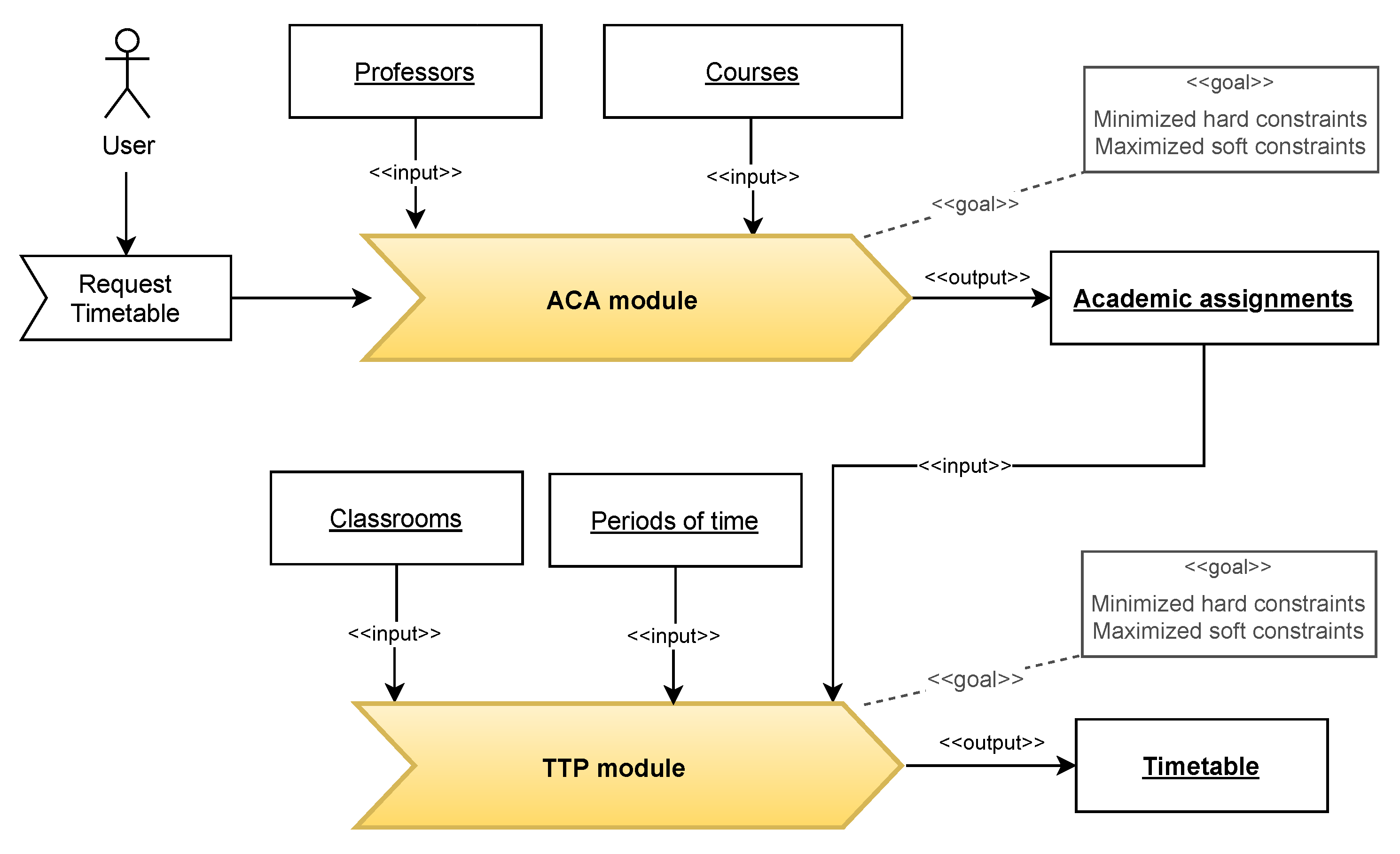
3. Modeling the Timetabling Problem

Each semester, the administrative staff at the UJAT-DACyTI builds a timetable that satisfies as many constraints as possible. The timetabling process is currently done manually during a period in the range of weeks with a considerable working hours cost. Specifically at our institution, the timetabling process is carried out in four stages:
  • The number of students who potentially want to take any course is determined through an online survey. This is known as the potential demand for each course.
  • Subsequently, the required courses are offered.
  • Next, each professor is asked for the list of courses they choose to teach in the following semester.
  • Using these data, the ACademic Assignments [ACA] (allocation of professors to courses) are made considering each professor’s particular constraints, such as research projects, popularization of science, and extension activities.
  • Finally, the TimeTabling Process [TTP] is performed.
Each stage involves a different amount of time and resources. In this research, we have modeled the last two stages of the process, that is, the constraints that are related to the timetabling problem. To describe these constraints, we designed OCL invariants from the domain model shown in Figure 1. The domain model includes the most representative elements of the timetabling problem, as well as specific attributes of the problem at UJAT:
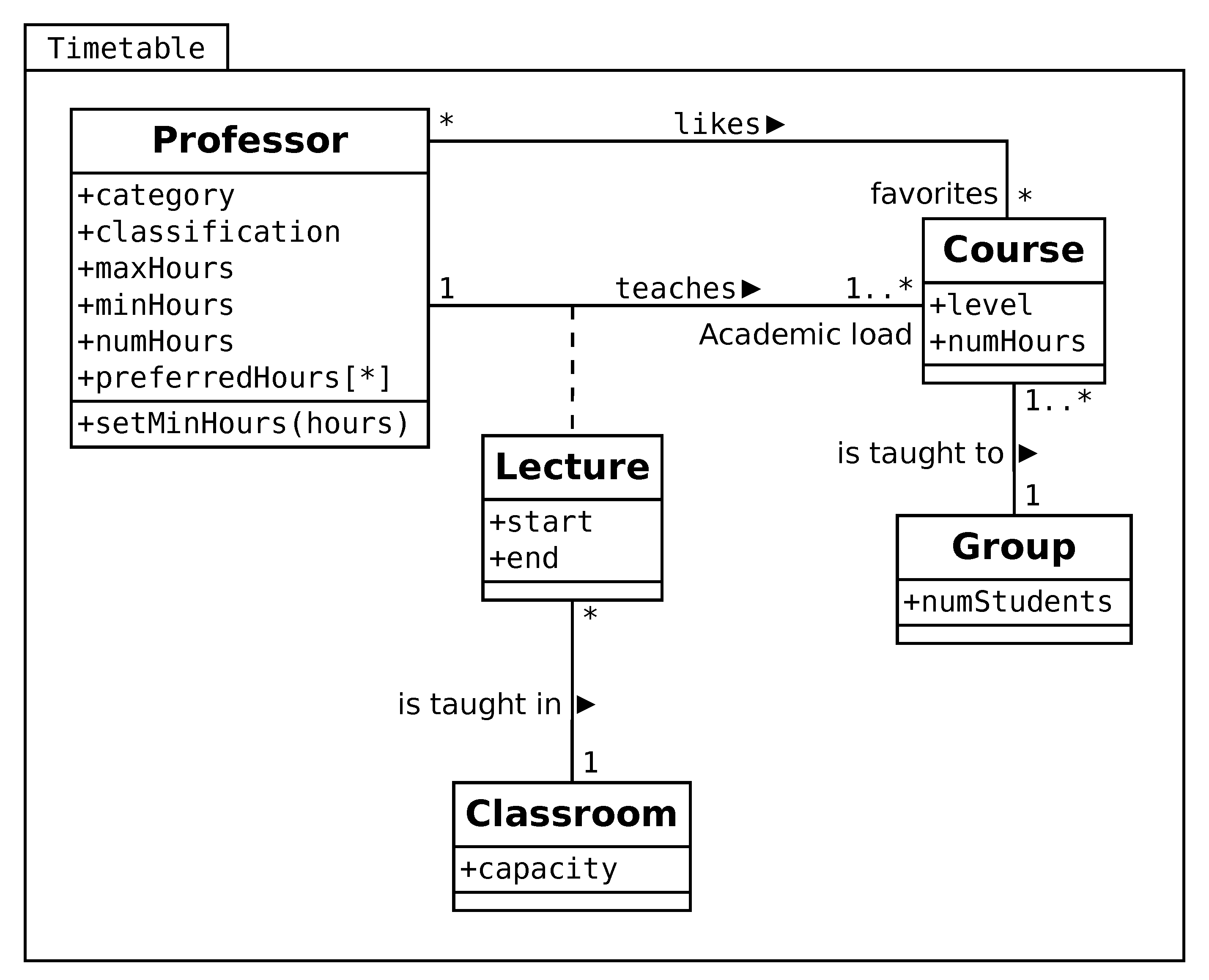
  • Professor: gives courses to groups of students. This entity has a predefined minimum and a maximum number of hours to teach during the semester, depending on her/his classification (visitor, emeritus, eventual, half-time, or full-time) and category (associate or titular).
  • Course: includes a number of hours in a week and a level (Undergraduate or Postgraduate).
  • Lecture: class given in a specific classroom during a certain period of time.
  • Group: number of students who receive classes in common.
  • Classroom: physical space with a specific capacity.
The Domain model of Figure 1 defines the following hard constraints that any valid timetable must satisfy:
  • A single teacher teaches a specific course.
  • A teacher must only teach one lecture at a time.
  • A lecture belongs to a particular course.
  • Lectures are taught in only one classroom at a time.
  • A lecture is given to a particular group.
These constraints are the typical hard constraints that are considered in the literature. However, our institution has more constraints and those cannot be represented in this type of model. Accordingly, the specific constraints of the timetabling problem at the DACyTI are detailed in the form of OCL invariants in the next section.

3.1. ACA Model

It is common to found detailed examples on how to create timetables [36,37,38,39,40]. However, at our institution there is a stage, called Academic assignments (ACA), which is usually not considered in the literature. This stage is a particularity of some educational institutions, in which the availability of teachers generally varies each semester, and there is no concept of professorship as in other institutions.
In this particular case, the Staff Regulation of the UJAT [41] establishes the relations between the university and academic personnel (categories, classifications, functions, income, and promotions), based on the terms that were established by Section VIII of Article 3 of the Mexican Constitution [42] and by the Organic Law of the UJAT [43].
The Staff Regulation establishes the labor restrictions that are formally described below. A valid ACA must meet the following hard constraints, subject to the model that is shown in Figure 1:
ACA-HC1. The courses taught at the DACyTI can be at the undergraduate or postgraduate level.
context Course
  inv: level=’Undergraduate’ or level=’Postgraduate’
ACA-HC2. Professors may have one of the following classifications: eventual, half-time, and full time, and, in an extraordinary situation, visitor and emeritus.
context Professor
    inv: classification=’Eventual’ or
       classification=’Half-Time’ or
       classification=’Full-Time’ or
       classification=’Visitor’ or
       classification =’Emeritus’
ACA-HC3. Professors may have one associate or titular category, each with levels A, B, or C.
context Professor
  inv: category=’Associate’ or category=’Titular’
  inv: level=’A’ or level=’B’ or level=’C’
ACA-HC4. The following attribute is defined for the correct validation of the total hours taught by a professor:
context Professor
  def: numHours:Integer = academicLoad.numHours->sum()
ACA-HC5. Constraints that are presented in the Staff Regulation regarding the minimum number of class hours for each professor are not absolute, so a convenient method to assign this value is:
context Professor::setMinHours(hours:Integer)
    inv: hours>0 and minHours<=maxHours
    body: minHours=hours
ACA-HC6. Eventual professors can teach at most 19 hours of class.
context Professor
  inv: classification=’Eventual’ implies maxHours=19
ACA-HC7. Associate Full-time professors who teach undergrad courses exclusively can teach no more than 25 hours of class.
context Professor
  inv: classification=’Full-time’ and category=’Associate’
    and academicLoad->forAll(c:Course | c.level=’Undergraduate’)
               implies maxHours=25
ACA-HC8. Associate full-time professors who teach at least one postgraduate course can teach no more than 20 hours of class.
context Professor
  inv: classification=’Full-time’ and category=’Associate’
    and academicLoad->exists(c:Course | c.level=’Postgraduate’)
               implies maxHours=20
ACA-HC9. Titular full-time professors who teach undergrad courses exclusively can teach no more than 20 hours of class.
context Professor
inv: classification=’Full-time’ and category=’Titular’
    and academicLoad->forAll(c:Course | c.level=’Undergraduate’)
             implies maxHours=20
ACA-HC10. Titular full-time professors who teach at least one postgraduate course can teach no more than 10 hours of class.
context Professor
  inv: classification=’Full-time’ and category=’Titular’
    and academicLoad->exists(c:Course | c.level=’Postgraduate’)
               implies maxHours=10
ACA-HC11. Associate half-time professors teaching exclusively undergrad courses can teach no more than 15 hours of class.
context Professor
  inv: classification=’Half-time’ and category=’Associate’
    and academicLoad->forAll(c:Course | c.level=’Undergraduate’)
               implies maxHours=15
ACA-HC12. Associate half-time professors who teach at least one postgraduate course can teach no more than 10 h of class.
context Professor
  inv: classification=’Half-time’ and category=’Associate’
    and academicLoad->exists(c:Course | c.level=’Postgraduate’)
               implies maxHours=10
ACA-HC13. Titular half-time professors who teach undergrad courses exclusively can teach no more than 10 h of class.
context Professor
  inv: classification=’Half-time’ and category=’Titular’
    and academicLoad->forAll(c:Course | c.level=’Undergraduate’)
               implies maxHours=10
ACA-HC14. Titular half-time professors who teach at least one postgraduate course can teach no more than five hours of class.
context Professor
  inv: classification=’Half-time’ and category=’Titular’
    and academicLoad->exists(c:Course | c.level=’Postgraduate’)
               implies maxHours=5
ACA-HC15. The number of lecture hours by each professor must not exceed the maximum hours established.
context Professor
  inv: numHours<=maxHours
ACA-HC16. The number of lecture hours by each professor must be greater than or equal to the minimum hours assigned.
context Professor
  inv: numHours>=minHours
Regarding the desirable conditions (soft constraints) for a valid ACA, we have:
ACA-SC1. Professors choose the courses that they would like to teach in the next semester. It would be desirable to satisfy the course preferences of each professor.
context Professor
  inv: academicLoad->intersection(favorites)->notEmpty()

3.2. TTP Model

Once the ACA is defined, the timetable is created. We divide each course into one-hour length lectures and then assign each lecture to a classroom during a period of time, satisfying the following hard constraints:
TTP-HC1. The time period for a lecture corresponds to 1 hour. The number of hours of each course must be assigned to the same number of time periods.
context Course
  inv: numHours=lecture->size()
TTP-HC2. The period of time labeled as 0 corresponds to the start period of classes on Monday, and the period labeled as TOTAL_PERIODS represents the final time of the last session on Friday. Both the first and last hours are known as overflow areas, and this type of allocation is called a compact schedule [44].
context Lecture
  inv: start>=0 and start<TOTAL_PERIODS
TTP-HC3. TTP-HC3 When considering blocks of time of 1 hour, the initial time of a lecture must be less than the final time by one hour.
context Lecture
  inv: end=start+1
TTP-HC4. The capacity of the classroom must fit the number of students in the group that takes a lecture.
context Lecture
  inv: classroom.capacity >= academicLoad.group.numStudents
TTP-HC5. TTP-HC5 A group must not take more than one lecture at a time (for ease of definition, the invariant is associated with courses, as each course is tied to one and only one group).
context Course
  inv: lecture->forAll(
                l1:Lecture,l2:Lecture | l1<>l2 implies l1.start<>l2.start)
TTP-HC6. A professor must not teach more than one lecture at a time.
context Professor
  inv: lecture->forAll(
                l1:Lecture,l2:Lecture | l1<>l2 implies l1.start<>l2.start)
Regarding the soft constraints for this stage, we have considered:
TTP-SC1. In the DACyTI, the concept of morning or evening shift does not properly exist due to the flexible educational model [45]. In that sense, the professor’ shifts were modeled as preferences about the period of time they wished to teach their courses.
context Professor
  inv: preferredHours->includesAll( Lecture.start->asSet() )
TTP-SC2. In our model, time periods are considered to be blocks of one-hour length, so lectures of the same course scheduled during the same day must be in contiguous hours. The constant PERIODS_A_DAY, equivalent to TOTAL_PERIODS/five days a week, is used in this invariant.
context Lecture
  inv: let day= start div PERIODS_A_DAY in
         let lecturesPerDay= Lecture.allInstances()->
               select(academicLoad=self.academicLoad and
                 (start div PERIODS_A_DAY) = day)->
                    asSet()->sortedBy(start) in
                      lecturesPerDay->size() > 1 implies
                        lecturesPerDay->iterate(s; i:Integer=0 |
                          if i<lecturesPerDay->size()-1 and s.end=
                            lecturesPerDay->at(i+1).start
                          then i+1
                          else i
                          endif) = lecturesPerDay->size()
The complete specification along the model validation in the USE environment are publicly available at the Open Science Framework: https://osf.io/zuh3s/.

4. Solution Proposal

According to the previous section’s constraints, the solution to the timetabling problem at the DACyTI was divided into the ACA phase and the TTP phase. For both stages, the Tabu Search with Probabilistic Aspiration Criterion (TS-PAC) algorithm was implemented in order to find a feasible solution, i.e., feasible academic assignments and a feasible timetable, respectively.

4.1. ACA Solution

The Academic assignments (ACA) are generated in three stages: (1) the creation of an initial solution, (2) satisfaction of the hard constraints, and (3) maximizing the course preferences for each professor.
Before starting the optimization process, data preprocessing is performed in order to obtain useful information to improve the performance of the Tabu Search algorithm, and the data structures to facilitate satisfying the hard constraints are created:
  • n p = number of professors.
  • n c = number of courses.
  • C = { c 1 , , c n c } corresponds to the set of instances of entity Course.
  • P = { p 1 , , p n p } corresponds to the set of instances of entity Professor.
  • F n p × n c 
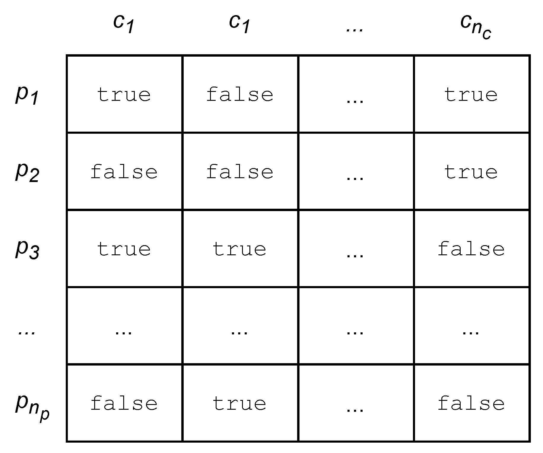
is the preference matrix where true represents professor p wants to teach the course c and false otherwise (Figure 2).
  • ACA n c 
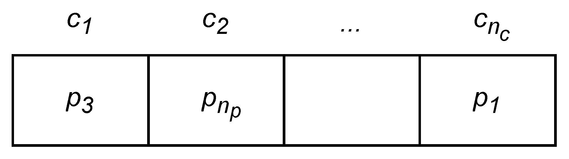
is a vector that corresponds to the solution (the academic assignments) where each cell c contains the assigned professor (Figure 3).

4.1.1. Creating an Initial Solution

A greedy algorithm makes a fair distribution of all the courses among the available professors, assigning to each of them at least one course within their preferences. In this way, the ACA starts balanced and attempts to satisfy at least one course for each professor.
In this stage, the maximum and the minimum number of hours per teacher is not validated; we only get ensured that each course has an assigned professor.

4.1.2. Satisfying Hard Constraints

This stage consists of satisfying the hard constraints that may exist in the solution generated in the previous stage. The objective function to optimize during this stage is:
Min . z = a c a h c 1 + a c a h c 2
where:
a c a h c 1 is the sum of unsatisfied constraints ACA-HC15.
a c a h c 2 is the sum of unsatisfied constraints ACA-HC16.
In order to satisfy the hard constraints, the TS-PAC algorithm uses a neighborhood that consists of random swaps between two professors; those with a higher academic load than the allowed against those with a less academic load than the corresponding one:
ACA - Neighborhood h c 1 = p , p p , p P | p . numHours > p . maxHours , p . numHours < p . minHours , p p
An additional neighborhood ACA - Neighborhood h c 2 = p x , p , helps the TS-PAC to escape from local optimum, adding some perturbation to the current solution. It consists of random swaps of courses between a professor causing constraint ( p x ) and a professor with a valid academic load ( p ).
The TS-PAC selects as the best element of neighborhood ACA - Neighborhood h c 1 the tuple that minimizes the highest number of hard constraints, when considering tabu elements and the aspiration criteria defined in Equation (9). The objective function of Equation (10) is minimization, so GOAL = 0 . If the search gets stuck in a local minimum, then an element from ACA - Neighborhood h c 2 is randomly selected to add perturbation to the current solution.
This stage ends when all hard constraints are satisfied, although this may not always be possible, as we will show in Section 5.

4.1.3. Soft Constraints: Maximizing Professors’ Course Preferences

The objective function of this stage is to maximize the preferences in the courses that are assigned to professors, without violating any of the hard constraints satisfied in the previous stage:
Max . z = a c a s c subject to : a c a h c 1 = 0 a c a h c 2 = 0
where:
a c a s c is the sum of the professors’ preferences, as defined in ACA-SC1.
a c a h c 1 and a c a h c 2 correspond to the hard constraints described in the objective function of Equation (10).
The neighborhood designed for this stage consists of swaps of professors between a couple of courses, selecting teachers who do not have any preferred course in their academic load, but do have some favorite course:
ACA - Neighborhood s c 1 = c , c c , c C | | c . professor . favorites | > 0 , c . professor . favorites c . professor . academicLoad = ϕ , | c . professor . favorites | > 0 , c . professor . favorites c . professor . academicLoad = ϕ , c . professor c . professor
An additional neighborhood ACA - Neighborhood s c 2 = p x , p adds some perturbation to the current solution, randomly swapping courses between two professors ( p x and p ).
The TS-PAC selects as the best element of the neighborhoods the tuple that maximizes the professor’s preferences, when considering tabu elements and the aspiration criterion defined in Equation (9). The objective function of Equation (11) is maximization: all of the professors with a favorite course in his/her Academic load, so we set GOAL to n p .

4.2. TTP Solution

During this phase, the same three-stage strategy is used: (1) the creation of an initial solution, (2) satisfaction of the hard constraints, and (3) maximizing professors’ shift preferences along with the number of lectures taught on the same day in contiguous hours.
First, data preprocessing is performed in order to create the necessary data structures used during the search process:
  • n r = number of classrooms.
  • n g = number of groups.
  • n l = number of lectures.
  • R = { r 1 , , r n r } corresponds to the set of instances of entity Classroom.
  • G = { g 1 , , g n g } corresponds to the set of instances of entity Group.
  • L = { l 1 , , l n l } corresponds to the set of instances of entity Lecture.
  • H n p × TOTAL _ PERIODS 
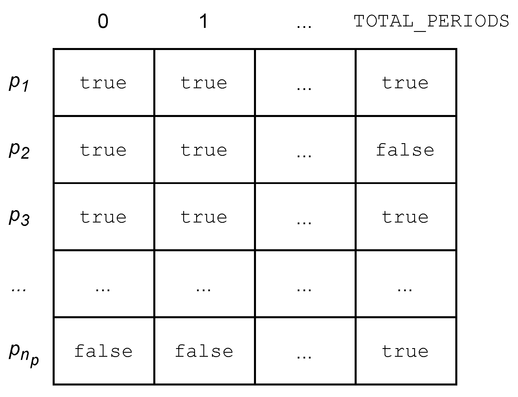
is a matrix where true represents that professor p desires to teach during that period of time, and false otherwise (Figure 4).
  • TTP n r × TOTAL _ PERIODS 
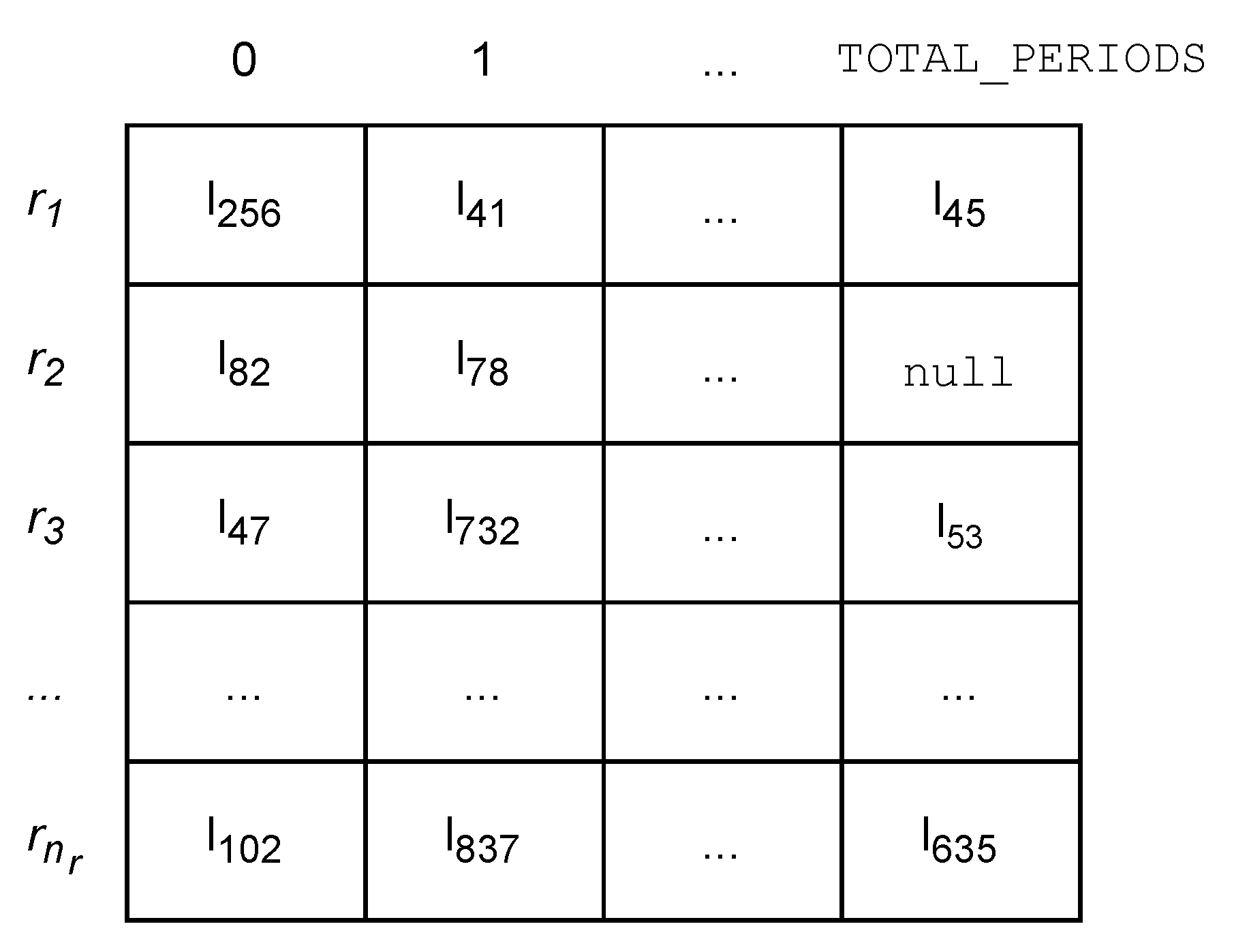
is a matrix corresponding to the solution (the timetable), where each cell corresponds to a lecture or null otherwise. This data structure has the advantage of automatically satisfying constraints of type TTP-HC2 and TTP-HC3, while facilitating the evaluation of the remaining constraints (Figure 5).

4.2.1. Creating an Initial Solution

A greedy algorithm generates the initial solution, fully solving constraints of type TTP-HC1 assigning the most professors in their shift of preference (constraint TTP-SC1) and avoiding lectures in non-contiguous time periods as much as possible during the same day (constraint TTP-SC2).

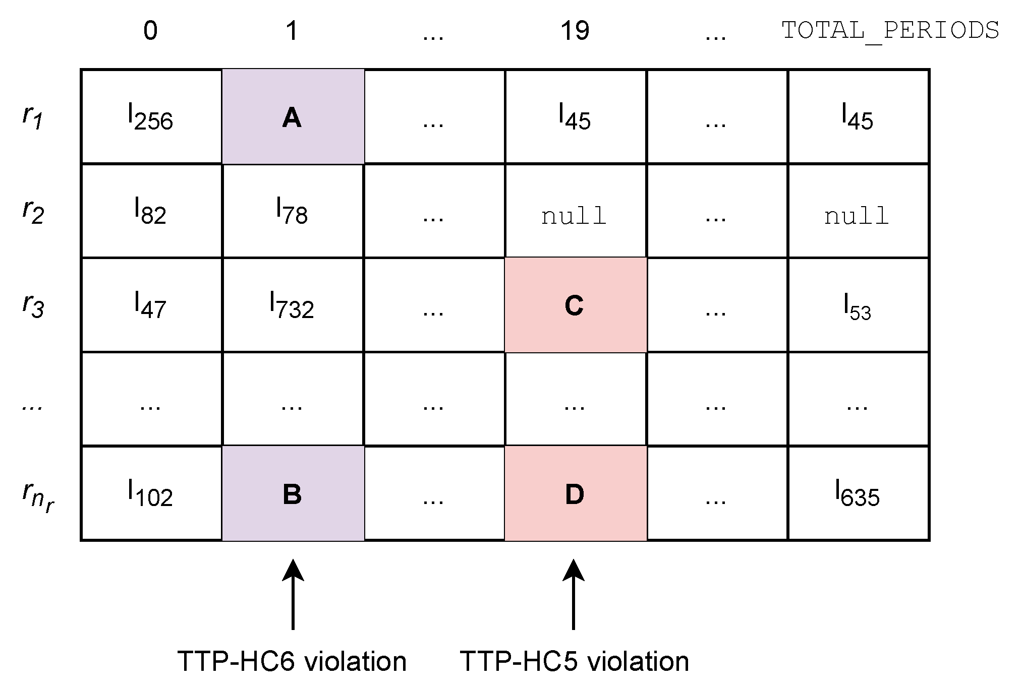
4.2.2. Satisfying Hard Constraints

During this stage, the remaining hard constraints in the initial solution are satisfied without considering the soft constraints. The objective function to optimize is:
Min . z = t t p h c 4 + w · ( t t p h c 5 + t t p h c 6 )
where:
t t p h c 4 is the sum of unsatisfied constraints TTP-HC4.
t t p h c 5 is the sum of unsatisfied constraints TTP-HC5.
t t p h c 6 is the sum of unsatisfied constraints TTP-HC6.
w is a positive constant that is sufficiently large to give more weight to constraints of type TTP-HC5 and TTP-HC6.
In Equation (12) we want to minimize the total number of hard constraints; however, priority is given to constraints of type TTP-HC5 and TTP-HC6 (a group and a professor must not take more than one lecture at a time), since most of the classrooms are big enough to fit groups (TTP-HC4).
Three neighborhoods are used at this stage, corresponding to random swaps of lectures. The following neighborhood scheme aims to minimize constraints of type TTP-HC4 (classroom capacity fits the number of students of a group):
TTP - Neighborhood h c 1 = l , l l , l L | l . classroom . capacity < l . course . group . numStudents , l . classroom . capacity > l . course . group . numStudents
Another neighborhood scheme that aims to minimize the constraints of type TTP-HC5 is (a group must not take more than one lecture at a time):
TTP - Neighborhood h c 2 = l , l l , l L | l . course = l . course , l . start = l . start , l l
The last neighborhood scheme helps to minimize constraints of type TTP-HC6 (a professor must not teach more than one lecture at a time):
TTP - Neighborhood h c 3 = l , l r l , l L | l . professor = l . professor , l . start = l . start , l l
An additional neighborhood TTP - Neighborhood h c 4 = l x , l , helps the TS-PAC to escape from local optimum adding some perturbation to the current solution. It consists of random swaps of time periods between a lecture causing constraint ( l x ) and a lecture correctly scheduled ( l ).
The algorithm selects the best element among the four neighborhoods that minimize the highest number of hard constraints, when considering tabu elements and the aspiration criterion. The objective function of Equation (12) for this stage is minimization ( GOAL = 0 ), so the probability p of selecting a tabu movement depends on the value of INIT and f ( s i ) according to Equation (9).
For example, consider the following scenario where four lectures are scheduled:
Lecture A:Lecture B:Lecture C:Lecture D:
    professor p 1     professor p 1     professor p 27     professor p 54
    course c 35     course c 87     course c 1     course c 1
    start 1     start 1     start 19     start 19
    end 2     end 2     end 20     end 20
In Figure 6, we can notice how Lecture A and Lecture B violate constraint TTP-HC6, since both lectures have Professor p 1 in common. Similarly, Lectures C and D violate constraint TTP-HC5, since both lectures belong to the same Course c 1 and, hence, belong to the same Group.

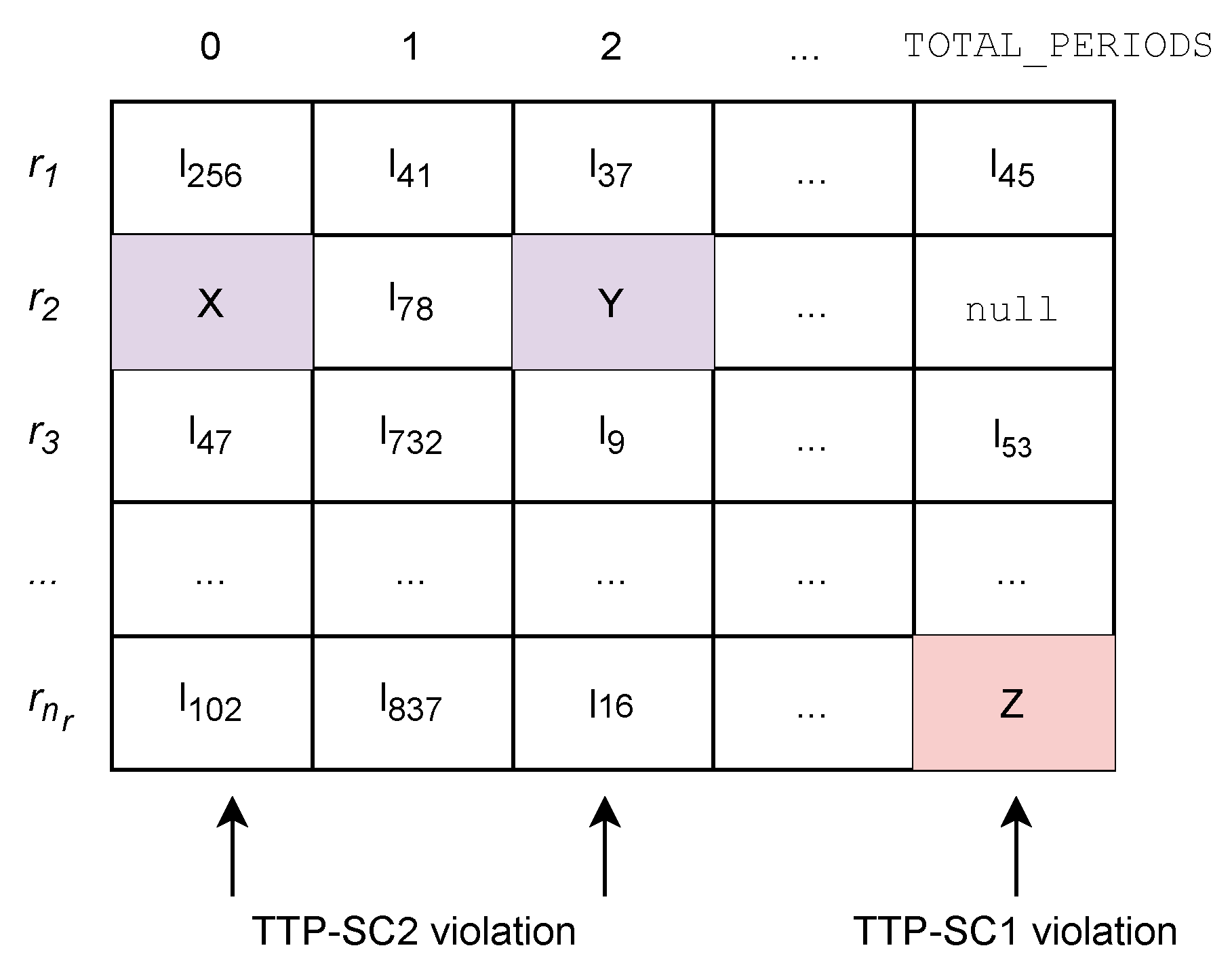
4.2.3. Soft Constraints: Maximizing Professors’ Shift Preferences and Contiguous Lectures

During this stage, we seek to maximize the shift preferences for each professor and, at the same time, maximize the number of lectures that are taught on the same day to be scheduled in contiguous hours. The objective function is:
Max . z = t t p s c 1 + ( w · t t p s c 2 ) subject to : t t p h c 4 = 0 t t p h c 5 = 0 t t p h c 6 = 0
where:
t t p s c 1 is the sum of professors preferences, as defined in TTP-SC1.
t t p s c 2 is the sum of courses with contiguous sessions in a day defined in TTP-SC2.
w is a positive constant that is sufficiently large to give more weight to constraints of type TTP-SC2.
t t p h c 4 , t t p h c 5 and t t p h c 6 correspond to the hard constraints described in the objective function of Equation (12).
In Equation (13), the goal is to maximize the professors’ shift preferences (constraint TTP-SC1) while reducing the number of lectures that are scheduled in non-contiguous hours of the same day (constraint TTP-SC2). It is desired to satisfy this last constraint to a larger extend; for this reason, we assigned a higher priority while using a weight constant.
For this stage, a couple of neighborhoods were designed to reduce the number of soft constraints. The first neighborhood consists of swaps of lectures, where the assigned professor has no hour preference satisfied (TTP-SC1):
TTP - Neighborhood s c 1 = l , l l , l L | l . start l . professor . preferredHours , l . start l . profesor . preferredHours , l l
The second neighborhood consists of swaps of lectures that are scheduled on the same day, but in non-contiguous hours (TTP-SC2):
TTP - Neighborhood s c 2 = l , l l , l L | l . course = l . course , l . start ÷ PERIODS _ A _ DAY = l . start ÷ PERIODS _ A _ DAY , | l . start l . end | > 0
An additional neighborhood TTP - Neighborhood s c 3 = l x , l adds some perturbation to the current solution, randomly swapping periods between two lectures ( p x and p ).
The TS-PAC selects the best element among the three neighborhoods that maximizes the professor’s preferences and contiguous lectures of the same course, when considering the tabu elements and the aspiration criterion. The objective function of Equation (13) for this stage is maximization, so the probability p of selecting a tabu movement depends on the value of GOAL and f ( s i ) according to Equation (9). In most of the experiments, we set GOAL = n l + n c .
For example, consider the following scenario where three lectures are scheduled:
Lecture X:Lecture Y:Lecture Z:Professor 77:
    professor p 51     professor p 51     professor p 77     category ⇒ Associate
    course c 23     course c 23     course c 96     classification ⇒ Full-Time
    start 0     start 2     start ⇒ TOTAL_PERIODS-1    preferredHours ⇒
    end 1     end 3     end ⇒ TOTAL_PERIODS        { 0 , 1 , 2 , 3 , 4 , , 33 }
In Figure 7, we can notice how Lecture X and Lecture Y violate constraint TTP-SC2, since the two lectures are scheduled in non-contiguous hours on the same day. Alongside, Lecture Z is violating constraint TTP-SC1, because it has been scheduled in a period of time not desired by the professor.

5. Tests and Results

We developed a software prototype to generate the timetable for the DACyTI, with one module for each of the two phases. We use the Open Java Development Kit, OpenJDK 8 [46] as a development platform, MariaDB [47] as the database management system, and our Tabu Search with Probabilistic Aspiration Criterion algorithm implementation over the OpenTS framework [48]. We made extensive use of the object-oriented programming (OOP) paradigm, organizing the prototype around objects, benefiting code reusability, scalability, and efficiency.

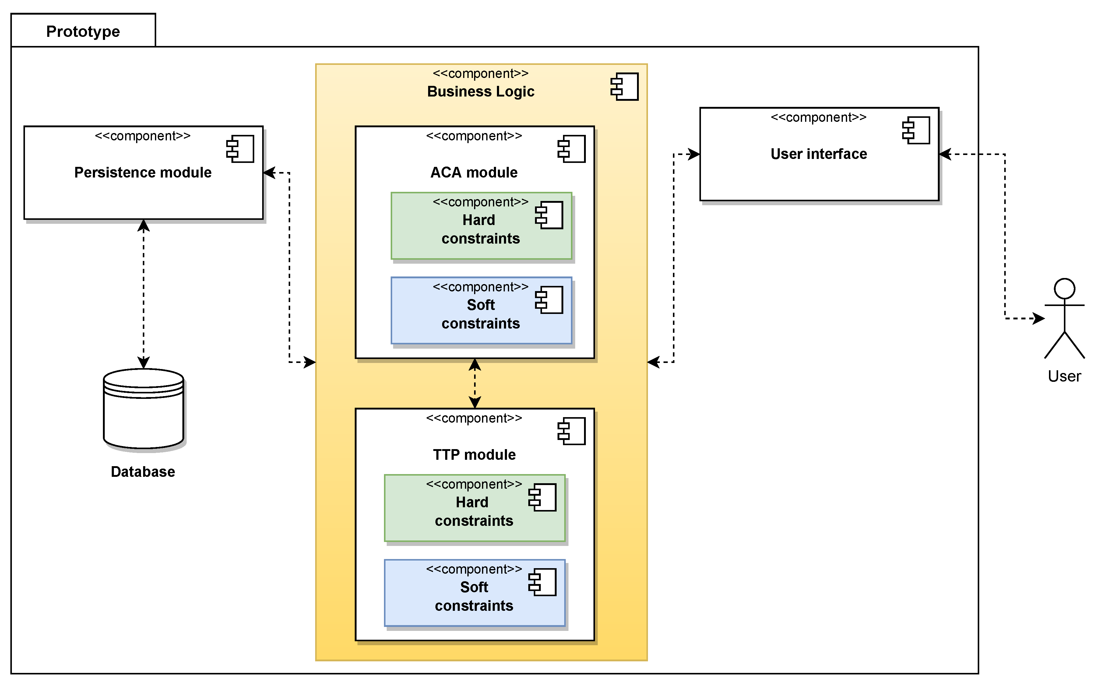
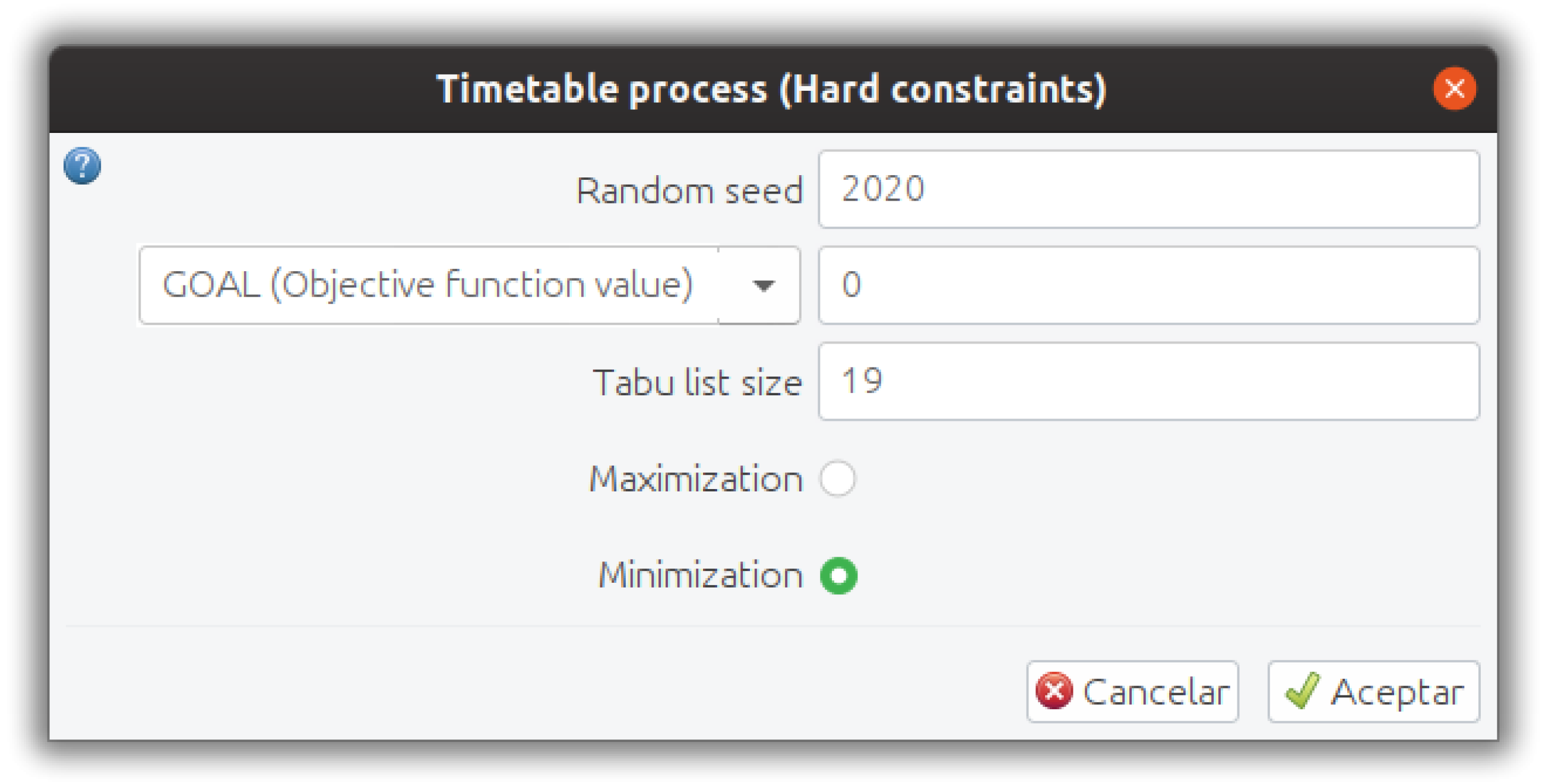
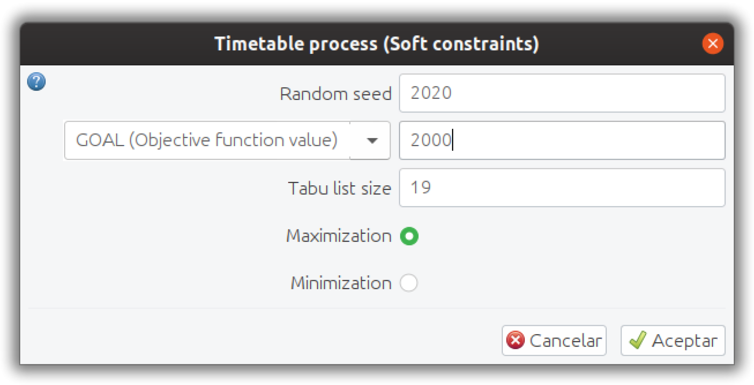
5.1. Software Prototype

Figure 8 shows the high-level design of our proposal, corresponding to the component diagram. It shows the static view of our prototype. The typical software layers (data, business, and presentation) are naturally separated into components with independent functionality.
Figure 9 shows the process diagram, where the components of the Bussiness logic are the central elements. This diagram shows the dynamic view of the prototype. The overall process starts when the event Request Timetable is fired. The ACA module inputs are the list of available professors and the list of courses. First, it minimizes the hard constraints and then maximizes the soft constraints. The resulting Academic assignments (ACA) are the inputs for the TTP module, along with the list of classrooms and periods of time. This module starts minimizing the hard constraints to continue with maximizing the soft constraints. The final output is the desired timetable.
Figure 10 and Figure 11 show the start window, used to configure the parameters of the algorithm: random seed, stop criterion (number of iterations, expected value in the objective function [ GOAL ], total seconds, or number of iterations with no improvement), and maximization or minimization option. Both of the figures show a sample parameter setting used in the soft and hard constraints for the ACA phase, respectively.
Figure 12 shows the search process for the ACA phase. It displays the academic assignments at each iteration, showing the courses for each professor and the information relative to each teacher’s lecture hours. Additionally, it shows the current value of the objective function. When the algorithm ends, the hard constraints stage, it displays a dialogue box with the resulting ACA, which can be a feasible solution or a solution with a set of assignments that violate some hard constraints. The user must manually select to continue with the soft constraints stage or return to the configuration window to start the search again. At any time, it is possible to pause the search process and save the obtained ACA so far. At the end of the soft constraints stage, the resulting ACA is displayed.
Once the Academic assignments (ACA) are generated, the timetable phase starts. Figure 13 and Figure 14 serve to configure the algorithm’s parameters in the TTP phase (same parameters as in the ACA phase). Both figures show a sample configuration used in the soft and hard constraints for the TTP phase, respectively.
Figure 15 shows the search process for the TTP phase. It displays the timetable details: course, professor, classroom, day, and time, as well as the current value of the objective function. The user can pause the search process and see the number of constraints left and the elapsed time. Once the hard constraints stage has been completed, the resulting timetable is displayed, which can be a feasible solution or a timetable that violates some hard constraints. As in the ACA phase, the user must decide to continue to the soft constraints stage or return to the configuration window in order to start the search again. At any time, it is possible to pause the process and save the obtained timetable so far. At the end of the soft constraints stage, the resulting timetable is displayed.

5.2. Experiments

The tests include two real semesters at the DACyTI with different characteristics. We conducted the experiments on an Alienware M17x laptop with Intel Core i7@2GHz processor, 16GB in RAM, and Ubuntu 18.04 64-bit operating system. The Tabu Search with Probabilistic Aspiration Criterion (TS-PAC) parameter configuration for both school periods is:
  • Start solution: through of a greedy algorithm. Different approaches to build an initial solution were used for the ACA phase hard constraints, ACA phase soft constraints, TTP hard constraints, and TTP soft constraints.
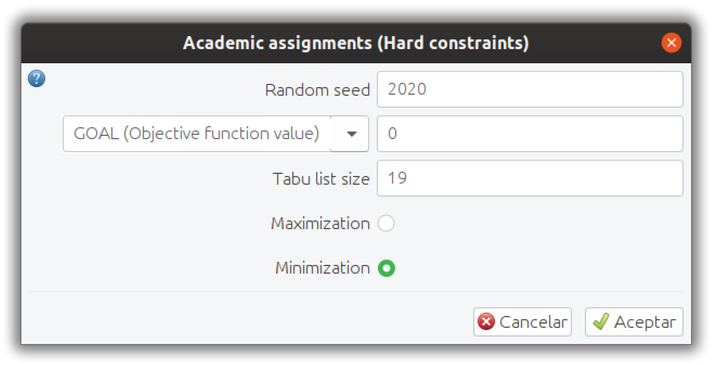
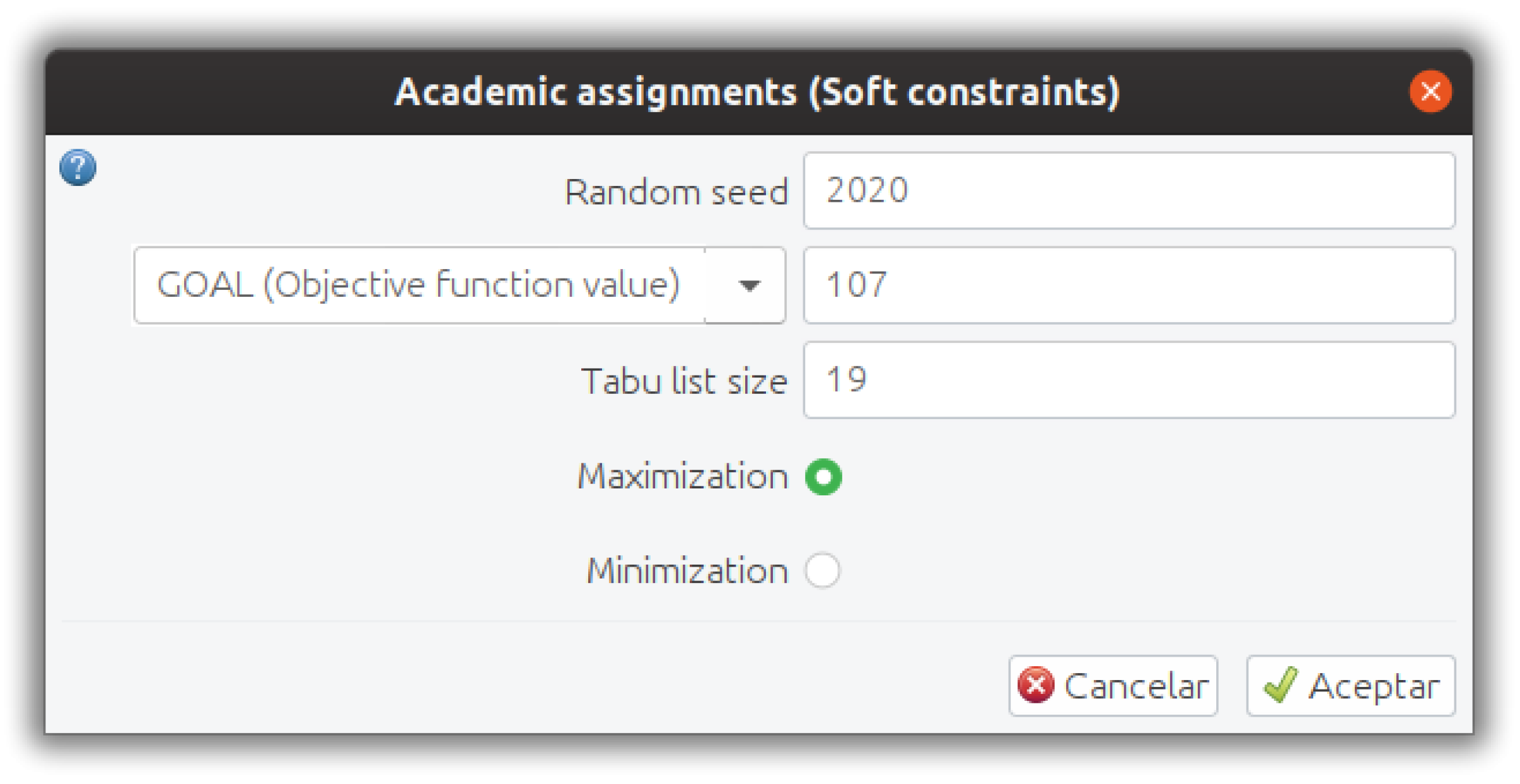
  • Random seed: a set of random numbers were generated using the random.org platform. The best seed value was 10,769,230.
  • Tabu list size: t = number of courses .
  • Neighborhood: different neighborhood structures were designed for each phase.
  • Aspiration criterion: the probabilistic aspiration criterion described in Section 2.3.
  • Stop criterion: variable, since different objective functions were defined for each phase. Additionally, we had to relax hard constraints in order to obtain a feasible solution.

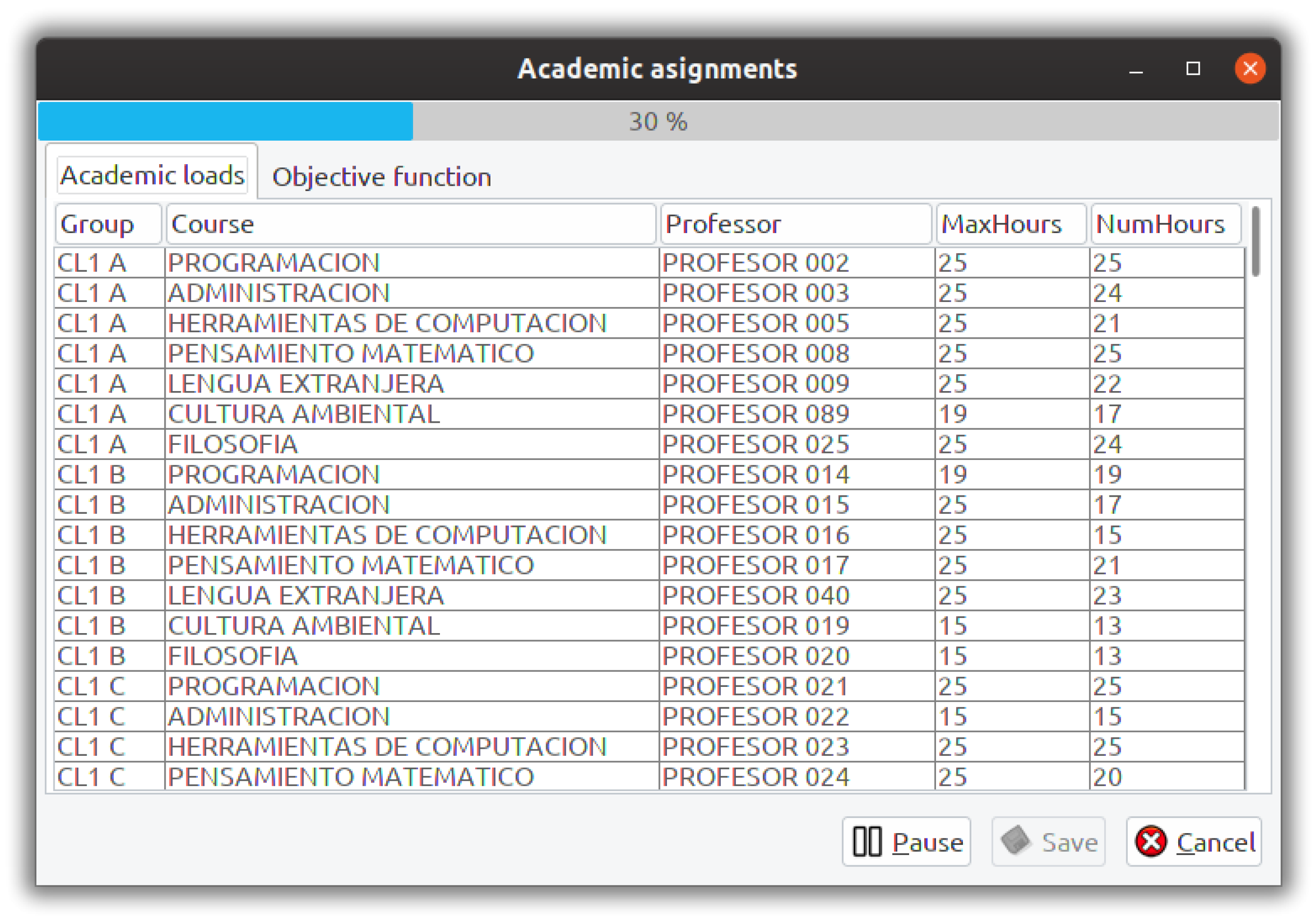
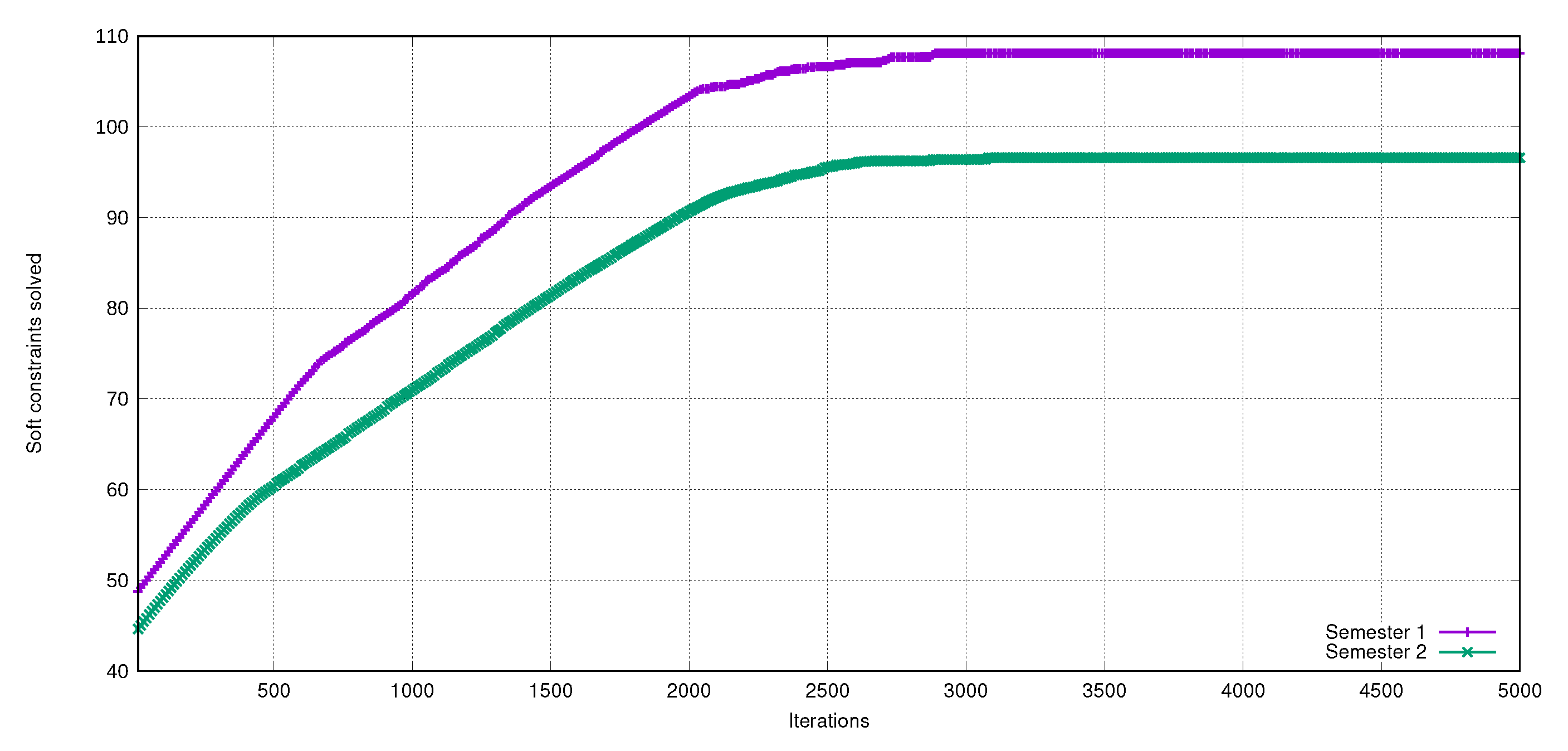
5.3. Results for the ACA Phase

Table 1 shows the data related to the ACA for the two test semesters. Creating the Academic assignments (ACA) requires the number of available professors, the number of courses to be offered, and the list of courses that each professor would like to teach. Satisfying the hard constraints involves the correct assignment of courses within the limits of each professor’s number of hours. The soft constraint stage seeks to maximize the professors’s course preferences as a whole, i.e., assign each professor at least one course in his preferences.
It is important to mention that each semester may vary the number of professors (some might temporarily leave pursuing postgraduate studies, or ask for a temporary unpaid leave holding government positions). Similarly, the number of courses is the most variable data, because each semester may vary the number of students who graduated and admitted to the university.
The associated constraints to this phase are distributed among entities as follows. We can notice that most of the restrictions in this phase are related to professors:
  • Course: hard constraint ACA-HC1.
  • Professor: hard constraints ACA-HC2 to ACA-HC16 and soft constraint ACA-SC1.
The results detailed in Table 2 show the violated constraints by the best solution found by the TS-PAC. In both semesters, most of the hard constraints were satisfied, but we could not reach a solution with zero hard constraints violation. Constraint ACA-HC16 was, in all tests, violated, meaning that some professors had fewer hours assignment than the permissible minimum. Thus, we needed to relax this hard constraint in order to continue to the soft constraint stage.
There are two professors with no academic load for the first test semester, i.e., no assigned coursesm, since the ACA was completed without requiring the total number of available professors. This may give a hint that there may be more professors than the required in the Faculty. All of the professors had a favorite course assigned (except for the two professors with no academic load), meaning that all of the soft constraints (constraint ACA-SC1) were satisfied.
In the second test semester, the number of teachers with fewer hours than the limit rises to 31, but there were no professors with unassigned courses. The percentage of satisfying preferences decreases this semester, since the number of professors with course preferences also decreased.
The logarithmic scale graph presented in Figure 16 displays the TS-PAC performance when evaluating the hard constraints for both semesters. In both cases, we set the stop criterion to a maximum number of iterations. The aggressive approach of the algorithm is remarkable. BT-PAC fast convergence is particularly due to the neighborhoods selected and the probabilistic aspiration criterion’s intensification strategy. Overall, the BT-PAC behavior is similar in both tests. However, convergence in semester 1 leads to most of the constraints being satisfied.
Figure 17 shows the performance of the algorithm when solving the soft constraints stage. Again, the behavior of the algorithm is similar in both semesters. Given that the objective function for this stage is maximization (Equation (11)), it is desired to satisfy, as far as possible, the professors’ course preferences. In this case, the stop criterion is GOAL = n p (number of professors). From the plot, we can read that both curves, representing each of the test semesters, are progressive and continuous. The expected maximum value in the objective function represents all of the professors satisfied with a favorite course assigned, so the TS-PAC converges to an acceptable solution with a low computational cost.

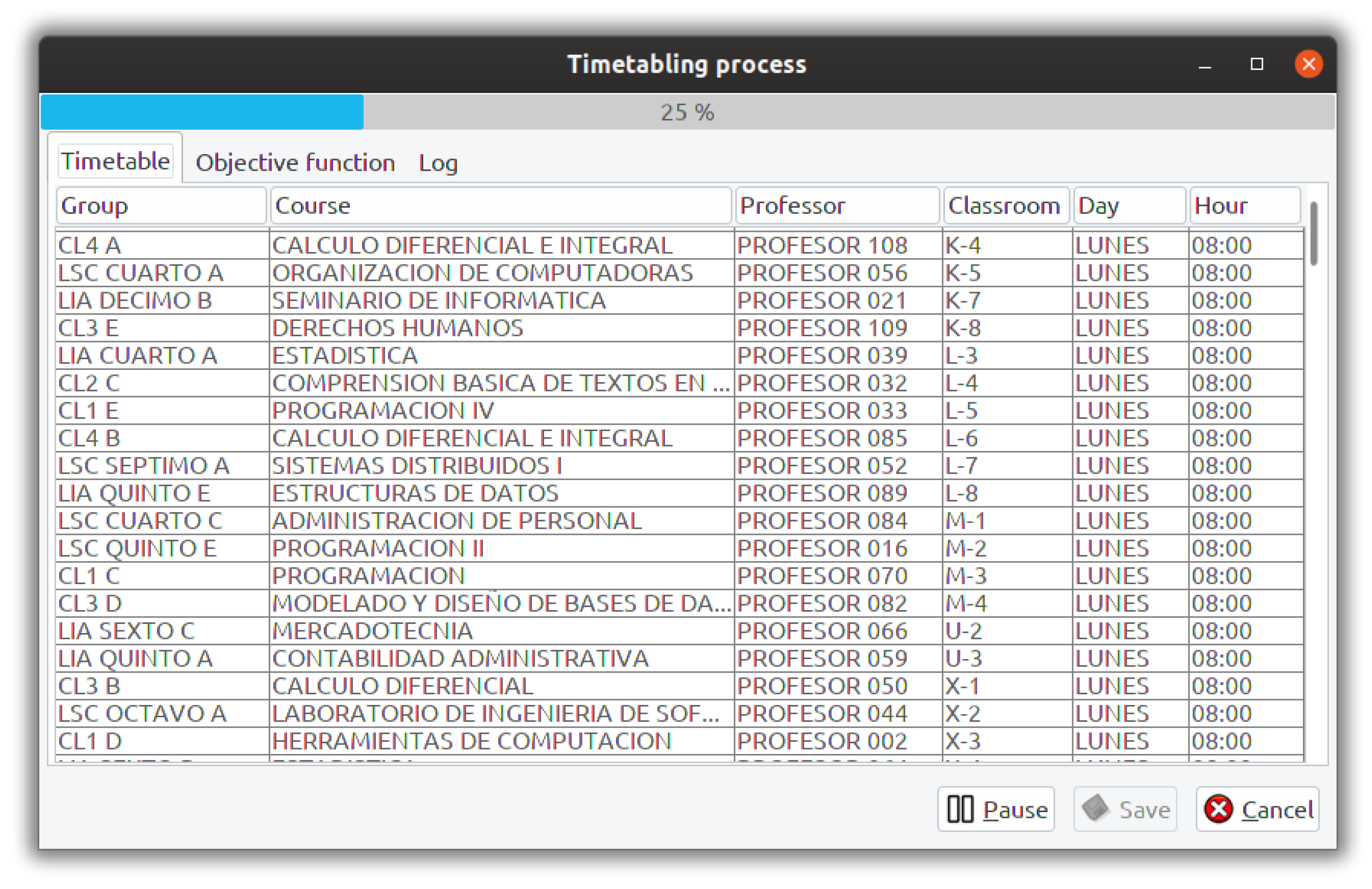
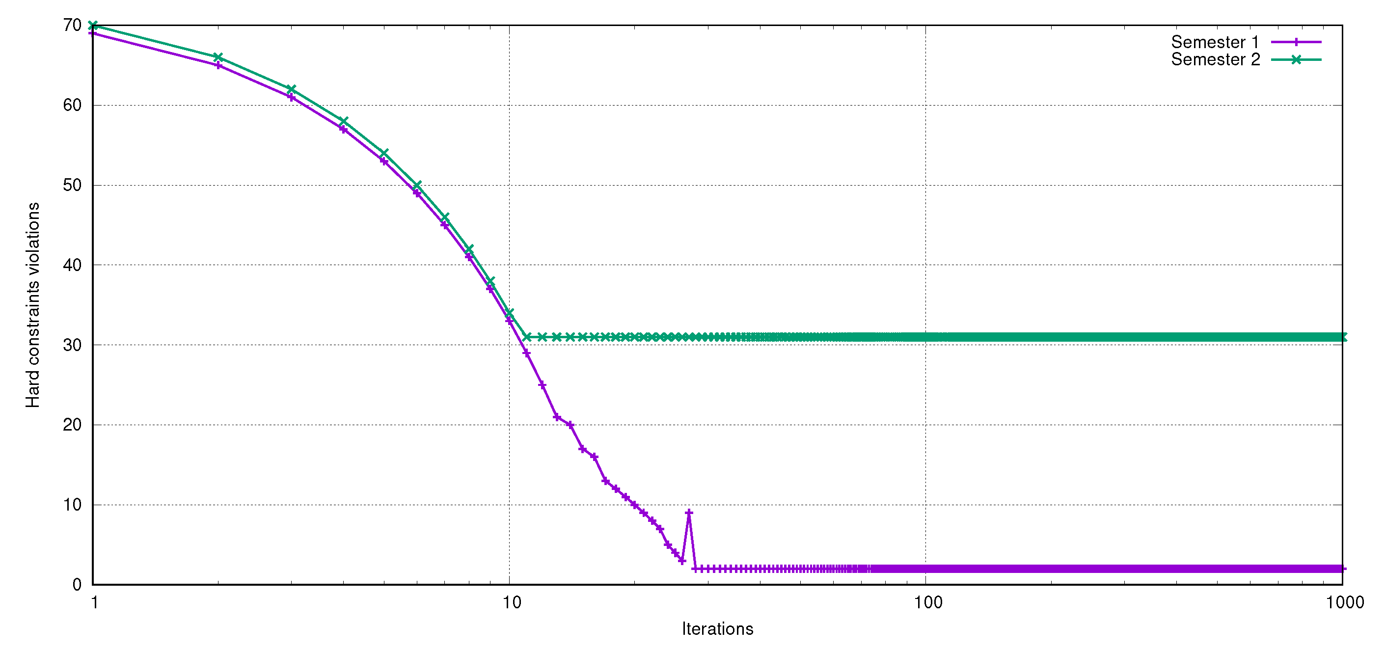
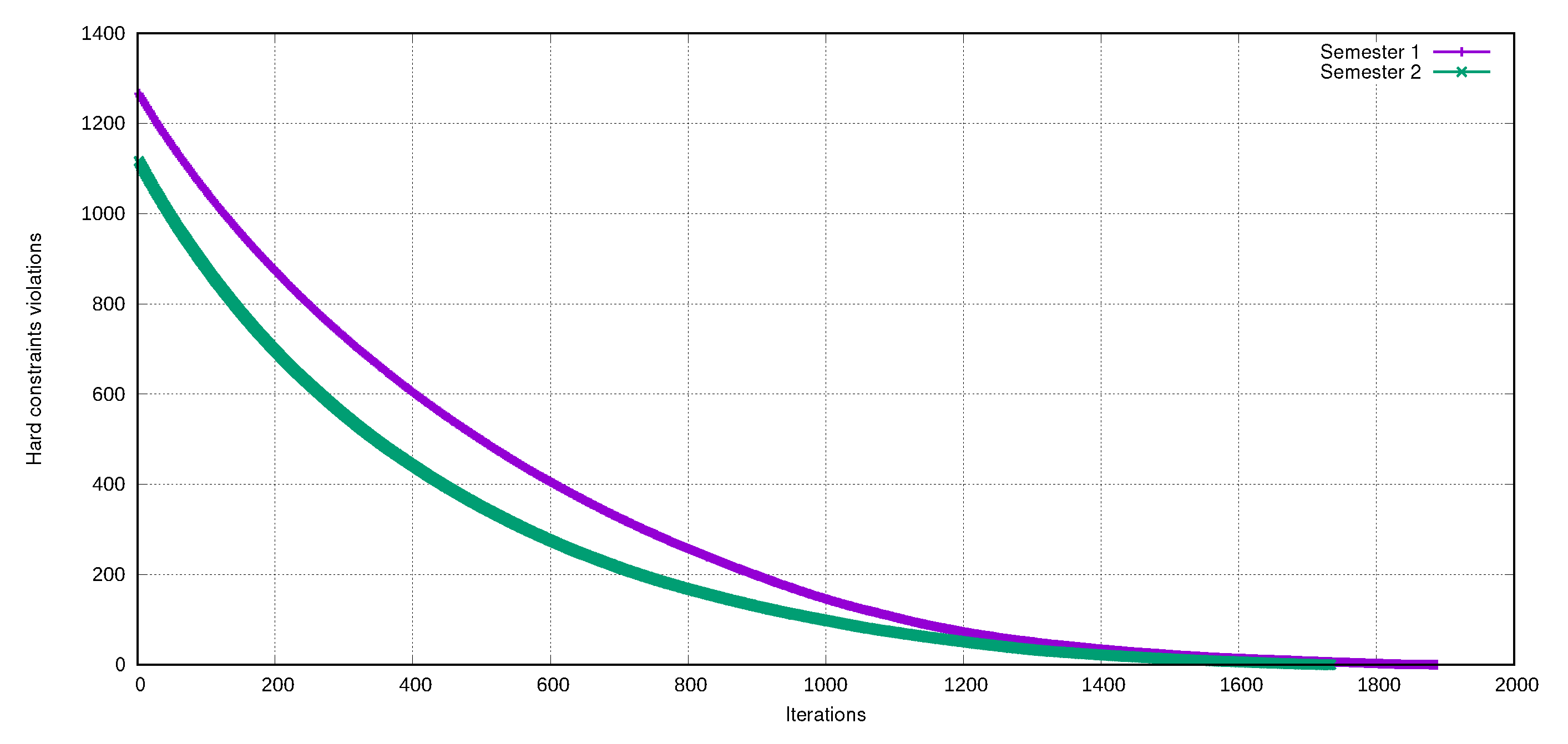
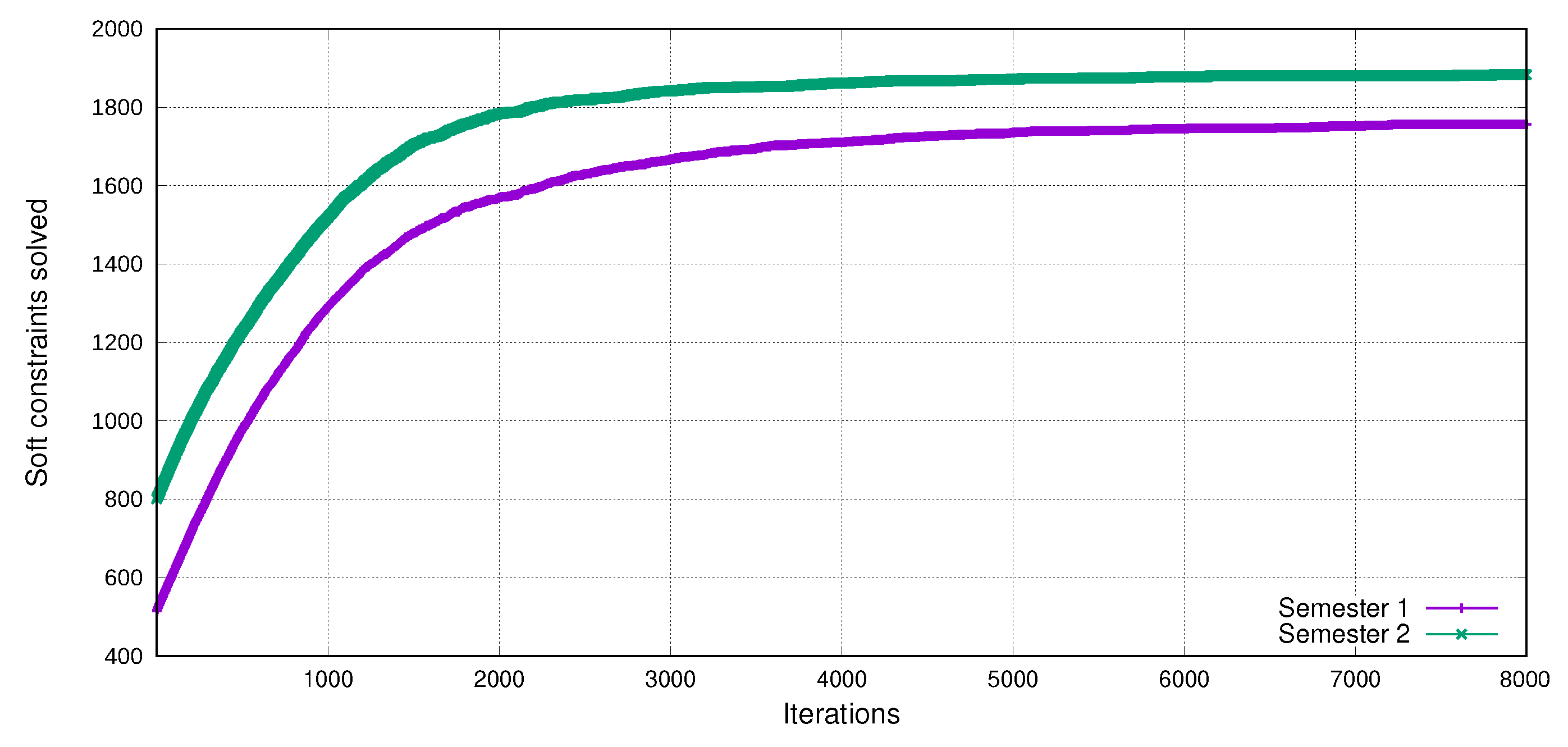
5.4. Results for the TTP Phase

Table 3 shows the data that were related to the TTP for the two test semesters. Creating a timetable requires the Academic assignments (ACA), i.e., each professor , course tuple, the number of groups, the available classrooms, and the number of periods of time. There is a main difference in both semesters: a reduction in the number of available time periods due to administrative issues. In the first semester, there were 12 periods of time per day (from 8 a.m. to 8 p.m.), but the second semester contains 10 periods per day (from 8 a.m. to 6 p.m.), both from Monday to Friday.
The associated constraints to this phase are distributed among entities, as follows. In this phase, we notice that more constraints are related to lectures:
  • Course: hard constraint TTP-HC1 and TTP-HC5.
  • Lecture: hard constraints TTP-HC2, TTP-HC3, and TTP-HC4. Soft constraint TTP-SC2.
  • Professor: hard constraint TTP-HC6 and soft constraint TTP-SC1.
The results for this stage are shown in Table 4. It is worth mentioning that none of the hard constraints considered are violated. All of the lectures were scheduled in a single period of time in a proper classroom, avoiding clashes. Regarding hard constraint TTP-HC4, it was easy to satisfy the constraint, because most of the classrooms are large enough to hold most of the courses.
Concerning soft constraints, the number of non-contiguous lectures on the same day were eliminated for both semesters (soft constraint TTP-SC2); this was our priority constraint. We also wanted to maximize the scheduling of lectures within each professor’s hour preferences, which was achieved in most cases (soft constraint TTP-SC1).
Figure 18 and Figure 19 show the performance of the TS-PAC when solving the hard constraints stage (minimization) and the soft constraints stage (maximization). We can notice that the behavior of the algorithm is very similar for both semesters. In the minimization stage (hard constraints), we set the stop criterion to GOAL = 0 , as achieved in both semesters. For the maximization stage (soft constraints), the stop criterion was set to a maximum number of iterations.
According to the results that were obtained in the two test cases, we can claim that the Tabu Search with Aspiration Criterion algorithm effectively solves the timetabling problem at the DACyTI.

6. Conclusions

The timetabling process is a complex problem, because it is not usually possible to find an optimal solution in a reasonable time, mainly due to the constraints of the problem and the many possible combinations of its intrinsic elements.
In that sense, the proposal of a formal model representing the specific constraints of the University Course Timetabling Problem (UCTP) at a Latin American university is the first contribution of this research. The inherent hard and soft constraints of the problem were described using the UML and the OCL, both software specification languages considered as standard. More importantly, the proposed model is not tied to any particular solution strategy. We consider that our model is sufficiently flexible to allow for new constraints over the same domain, removing or modifying the existing ones. Even new entities, like substitute teachers or the concept of university chair, can be straightforwardly added.
In the literature, there are few cases in which the UCTP is described in two phases that we have called Academic assignments (ACA) and Timetable process (TTP). Separating our problem at the DACyTI into the ACA and TTP phases allows for us to tackle the problem by: (1) modeling specific constraints for each phase, (2) divide each phase into hard and soft constraints stages, specifying two objective functions for each phase, and (3) the design of specific neighborhoods for the Tabu Search algorithm in each phase. Besides, this two-phases technique represents a similar paradigm to the know-how of the personnel responsible for the timetabling process at our university, so it may optimize the manual work, so our prototype may help to optimize the manual work currently done.
We relied on the Tabu Searchm because it is a fast algorithm, easy to tune, and it allows a semi-deterministic search via the designed neighborhoods. In that sense, feasible timetables were generated in the order of minutes. We made a customization of the Tabu Search algorithm, the so-called Tabu Search with Probabilistic Aspiration Criterion (BT-PAC). The aspiration criterion is regularly not taken into account in the various variants of the Tabu Search algorithm presented in the literature. In this case, the proposed aspiration criterion allows for intensifying and diversifying the search in crucial situations, which improves the algorithm’s overall performance. Besides, Tabu Search can be easily implemented in an object-oriented programming language.
A multiplatform software prototype was developed to implement our proposal. This prototype was tested with two semesters of different characteristics in terms of the number of elements to be considered: professors, courses, and periods of time. In both semesters, quality solutions were obtained, satisfying most of the constraints. It is possible to adapt the prototype in order to solve the timetabling problem at other academic divisions of our university, or even in other universities with similar constraints. We exclusively used free software for the development of the prototype.
Among the future works, we have considered implementing a hybrid algorithm while using another metaheuristic in order to explore different areas of the solution space. It is also possible to design various neighborhood schemes to provide further diversity to the solutions generated by the algorithm. Regarding the software prototype, it is suggested to apply quality metrics and usability tests to enrich its functionality.
It is expected that the present model and proposed solution serve as a basis for modeling and solving other instances of the timetabling problem.

Author Contributions

O.C.-B.: Conceptualization, Methodology, Software, Writing- Original draft preparation. J.H.-T.: Data curation, Software. B.H.-O.: Validation, Investigation. J.C.-R.: Writing-Reviewing and Editing. All authors have read and agreed to the published version of the manuscript.

Funding

This research received no external funding.

Acknowledgments

To CONACYT (Ministry of Science in México) for supporting the National System of Researchers (SNI) program.

Conflicts of Interest

The authors declare no conflict of interest.

Abbreviations

The following abbreviations are used in this manuscript:
ACAAcademic assignments
DACyTIDivisión Académica de Ciencias y Tecnologías de la Información
OCLObject Constraint Language
TS-PACTabu Search with Probabilistic Aspiration Criterion
TTPTimetabling problem
UJATUniversidad Juárez Autónoma de Tabasco
UCTPUniversity Course Timetabling Problem
UMLUnified Modeling Language

References

  1. Cooper, T.B.; Kingston, J.H. The complexity of timetable construction problems. In Practice and Theory of Automated Timetabling; Burke, E., Ross, P., Eds.; Springer: Berlin/Heidelberg, Germany, 1996; pp. 281–295. [Google Scholar]
  2. Cruz-Chávez, M.; Flores-Pichardo, M.; Martínez-Oropeza, A.; Moreno-Bernal, P.; Cruz-Rosales, M. Solving a Real Constraint Satisfaction Model for the University Course Timetabling Problem: A Case Study. Math. Probl. Eng. 2016, 2016, 14. [Google Scholar] [CrossRef]
  3. Mejía Caballero, J.; Paternina Arboleda, C. Asignación de Horarios de Clases universitarias mediante Algoritmos Evolutivos (Allocation of class schedules using evolutionary algorithms). Rev. Educ. Ing. 2010, 5, 140–149. [Google Scholar] [CrossRef]
  4. Pereira, V.; Gomes Costa, H. Linear Integer Model for the Course Timetabling Problem of a Faculty in Rio de Janeiro. Adv. Oper. Res. 2016, 2016. [Google Scholar] [CrossRef]
  5. Gotlieb, H. The construction of class-teacher timetables. In Proceedings of IFIP Congress 62; Popplewell, C., Ed.; Information Processing 62: Munich, Germany, 1963; pp. 73–77. [Google Scholar]
  6. Saviniec, L.; Santos, M.O.; Costa, A.M. Parallel local search algorithms for high school timetabling problems. Eur. J. Oper. Res. 2018, 265, 81–98. [Google Scholar] [CrossRef]
  7. De Werra, D. An introduction to timetabling. Eur. J. Oper. Res. 1985, 19, 151–162. [Google Scholar] [CrossRef]
  8. Rudová, H.; Müller, T.; Murray, K. Complex university course timetabling. J. Sched. 2011, 14, 187–207. [Google Scholar] [CrossRef]
  9. Schaerf, A. A Survey of Automated Timetabling. Artif. Intell. Rev. 1999, 13, 87–127. [Google Scholar] [CrossRef]
  10. Burke, E.K.; Mareček, J.; Parkes, A.J.; Rudová, H. Decomposition, reformulation, and diving in university course timetabling. Comput. Oper. Res. 2010, 37, 582–597. [Google Scholar] [CrossRef] [Green Version]
  11. Chen, M.; Tang, X.; Song, T.; Wu, C.; Liu, S.; Peng, X. A Tabu search algorithm with controlled randomization for constructing feasible university course timetables. Comput. Oper. Res. 2020, 123, 105007. [Google Scholar] [CrossRef]
  12. Chiorean, D.; Petraşcu, V.; Ober, I. Using Constraints in Teaching Software Modeling. In Models in Software Engineering; Kienzle, J., Ed.; Springer: Berlin, Germany, 2012; pp. 25–39. [Google Scholar]
  13. Booch, G.; Rumbaugh, J.; Jacobson, I. The Unified Modeling Language User Guide; Addison-Wesley: Boston, MA, USA, 2005. [Google Scholar]
  14. Hofrichter, O.; Hamann, L.; Gogolla, M.; Steimke, F. The secret life of OCL constraints. In Proceedings of the 12th Workshop on OCL and Textual Modelling-OCL ‘12; ACM Press: New York, NY, USA, 2012. [Google Scholar] [CrossRef] [Green Version]
  15. Cabot, J.; Gogolla, M. Object Constraint Language (OCL): A Definitive Guide. In Formal Methods for Model-Driven Engineering: 12th International School on Formal Methods for the Design of Computer, Communication, and Software Systems, SFM 2012, Bertinoro, Italy, 18–23 June 2012; Advanced Lectures; Springer: Berlin, Germany, 2012; pp. 58–90. [Google Scholar] [CrossRef] [Green Version]
  16. Ziemann, P.; Gogolla, M. Validating OCL Specifications with the USE Tool: An Example Based on the BART Case Study. Electron. Notes Theor. Comput. Sci. 2003, 80, 157–169. [Google Scholar] [CrossRef] [Green Version]
  17. Larsson, D.; Mostowski, W. Specifying Java Card API in OCL. Electron. Notes Theor. Comput. Sci. 2004, 102, 3–19. [Google Scholar] [CrossRef] [Green Version]
  18. Garry, D.; Balfe, T. Experiences using OCL for business rules on financial messaging. In Proceedings of the 12th Workshop on OCL and Textual Modelling (OCL’12); ACM Press: New York, NY, USA, 2004; pp. 65–66. [Google Scholar] [CrossRef]
  19. Chávez-Bosquez, O.; Pozos-Parra, P. The Latin American laws of correct nutrition: Review, unified interpretation, model and tools. Comput. Biol. Med. 2016, 70, 67–79. [Google Scholar] [CrossRef] [Green Version]
  20. Gogolla, M.; Büttner, F.; Richters, M. USE: A UML-based specification environment for validating UML and OCL. Sci. Comput. Program. 2007, 69, 27–34. [Google Scholar] [CrossRef] [Green Version]
  21. Glover, F.; Laguna, M. Tabu Search, 1st ed.; Kluwer Academic Publishers: Norwell, MA, USA, 1997. [Google Scholar]
  22. Pirim, H.; Bayraktar, E.; Eksioglu, B. Tabu Search: A Comparative Study. In Tabu Search; InTechOpen: London, UK, 2008. [Google Scholar] [CrossRef] [Green Version]
  23. Kergosien, Y.; Lenté, C.; Piton, D.; Billaut, J.C. A tabu search heuristic for the dynamic transportation of patients between care units. Eur. J. Oper. Res. 2011, 214, 442–452. [Google Scholar] [CrossRef]
  24. Cunha, V.; Mantovani, J. Planning And Project Of Medium Voltage Electric Power Distribution Systems. IEEE Latin Am. Trans. 2016, 15, 2298–2308. [Google Scholar] [CrossRef]
  25. Balliauw, M.; Herremans, D.; Palhazi Cuervo, D.; Sörensen, K. Mathematics and Computation in Music: 5th International Conference, MCM 2015, London, UK, 22–25 June 2015; Chapter Generating Fingerings for Polyphonic Piano Music with a Tabu Search Algorithm; Springer International Publishing: Berlin, Germany, 2015; pp. 149–160. [Google Scholar] [CrossRef]
  26. Glover, F. Tabu Search: A Tutorial. Interfaces 1990, 20, 74–94. [Google Scholar] [CrossRef] [Green Version]
  27. Gendreau, M. An Introduction to Tabu Search. In Handbook of Metaheuristics; Glover, F., Kochenberger, G.A., Eds.; Springer: Boston, MA, USA, 2003; pp. 37–54. [Google Scholar] [CrossRef]
  28. Xing, L.; Liu, Y.; Li, H.; Wu, C.C.; Lin, W.C.; Chen, X. A Novel Tabu Search Algorithm for Multi-AGV Routing Problem. Mathematics 2020, 8, 279. [Google Scholar] [CrossRef] [Green Version]
  29. Al-Tarawneh, H.; Ayob, M. Using Tabu search with multi-neighborhood structures to solve University Course Timetable UKM case study (faculty of engineering). In Proceedings of the 3rd Conference on Data Mining and Optimization, Putrajaya, Malaysia, 28–29 June 2011; pp. 208–212. [Google Scholar] [CrossRef]
  30. Hertz, A. Tabu search for large scale timetabling problems. Eur. J. Oper. Res. 1991, 54, 39–47. [Google Scholar] [CrossRef]
  31. Minh, K.N.T.T.; Thanh, N.D.T.; Trang, K.T.; Hue, N.T.T. Using Tabu Search for Solving a High School Timetabling Problem. In Advances in Intelligent Information and Database Systems; Springer: Berlin, Germany, 2010; pp. 305–313. [Google Scholar] [CrossRef]
  32. Oliva, C.; Ramírez, G. Algoritmo de tipo búsqueda tabú para un problema de programación de horarios universitarios vespertinos. INGE CUC 2013, 9, 58–65. [Google Scholar]
  33. Schaerf, A. Tabu Search Techniques for Large High-School Timetabling Problems. In Proceedings of the 13th National Conference on Artificial Intelligence (AAAI-96); AAAI Press/MIT Press: Portland, OR, USA, 1996; pp. 363–368. [Google Scholar]
  34. Chávez-Bosquez, O.; Pozos-Parra, P.; Gómez-Ramos, J. Búsqueda Tabú con Criterio de Aspiración Probabilístico aplicada a la Generación de Horarios Escolares (Tabu Search with Probabilistic Aspiration Criterion solving the timetabling problem). Rev. Mat. Teor. Apl. 2015, 22, 153–177. [Google Scholar] [CrossRef] [Green Version]
  35. Network, M. International Timetabling Competition. 2003. Available online: http://sferics.idsia.ch/Files/ttcomp2002/ (accessed on 16 September 2018).
  36. Müller, T.; Rudová, H.; Müllerová, Z. University course timetabling and International Timetabling Competition 2019. In Proceedings of the PATAT 2018: 12th International Conference of the Practice and Theory of Automated Timetabling; Burke, E., Di Gaspero, L., McCollum, B., Musliu, N., Özcan, E., Eds.; Online: Vienna, Austria, 2018; pp. 5–31. [Google Scholar]
  37. Kingston, J.H. Educational Timetabling. In Automated Scheduling and Planning: From Theory to Practice; Uyar, A.S., Ozcan, E., Urquhart, N., Eds.; Springer: Berlin, Germany, 2013; pp. 91–108. [Google Scholar] [CrossRef]
  38. Chen, R.M.; Shih, H.F. Solving University Course Timetabling Problems Using Constriction Particle Swarm Optimization with Local Search. Algorithms 2013, 6, 227–244. [Google Scholar] [CrossRef]
  39. Mockus, J.; Pupeikienė, L. On Multi-Start Algorithms for Optimization of High School Timetables. Informatica 2012, 23, 405–425. [Google Scholar] [CrossRef]
  40. Piechowiak, S.; Kolski, C. Towards a generic object oriented decision support system for university timetabling: An interactive approach. Int. J. Inf. Technol. Decis. Mak. 2004, 3, 179–208. [Google Scholar] [CrossRef]
  41. H. Consejo Universitario (University Council). Estatuto del Personal Académico (Academic Staff Regulations); Universidad Juárez Autónoma de Tabasco: Tabasco, Mexico, 1985. [Google Scholar]
  42. Secretaría de Gobernación (Ministry of the Interior). Constitución Política de los Estados Unidos Mexicanos (Mexican Constitution), 23rd ed.; Dirección General Adjunta del Diario Oficial de la Federación: Ciudad de México, Mexico, 2017. [Google Scholar]
  43. H. Congreso del Estado de Tabasco (Tabasco State Congress). Ley Orgánica de la Universidad Juárez Autónoma de Tabasco (UJAT Organic Law); Universidad Juárez Autónoma de Tabasco: Tabasco, Mexico, 1987. [Google Scholar]
  44. Müller, T.; Rudová, H. Real-life curriculum-based timetabling with elective courses and course sections. Ann. Oper. Res. 2016, 239, 153–170. [Google Scholar] [CrossRef]
  45. H. Consejo Universitario (University Council). Reglamento Escolar del Modelo Educativo Flexible (School Regulations of the Flexible Educational Model); Universidad Juárez Autónoma de Tabasco: Tabasco, Mexico, 2011. [Google Scholar]
  46. AdoptOpenJDK.net. AdoptOpenJDK - Prebuilt OpenJDK Binaries. 2019. Available online: https://adoptopenjdk.net (accessed on 16 April 2019).
  47. MariaDB Foundation. MariaDB Server. 2019. Available online: https://mariadb.org (accessed on 12 December 2019).
  48. Harder, R. OpenTS - Java Tabu Search. 2001. Available online: https://www.coin-or.org/Ots/ (accessed on 20 November 2018).
Figure 1. Unified Modeling Language (UML) domain model.
Mathematics 08 01833 g001
Figure 2. Professors’ preferences matrix.
Mathematics 08 01833 g002
Figure 3. The vector representing the Academic assignments.
Mathematics 08 01833 g003
Figure 4. Professors’ shift preferences matrix.
Mathematics 08 01833 g004
Figure 5. The matrix representing the timetable.
Mathematics 08 01833 g005
Figure 6. Example of hard constraints in a timetable.
Mathematics 08 01833 g006
Figure 7. Example of soft constraints in a timetable.
Mathematics 08 01833 g007
Figure 8. High-level diagram.
Mathematics 08 01833 g008
Figure 9. Process diagram.
Mathematics 08 01833 g009
Figure 10. A configuration of the Tabu Search with Probabilistic Aspiration Criterion (TS-PAC) parameters for the Academic assignments (ACA) phase (hard constraints).
Mathematics 08 01833 g010
Figure 11. A configuration of the TS-PAC parameters for the ACA phase (soft constraints).
Mathematics 08 01833 g011
Figure 12. Academic assignments: list of professors with assigned courses.
Mathematics 08 01833 g012
Figure 13. Sample configuration of the TS-PAC parameters for the timetable process (TTP) phase (hard constraints).
Mathematics 08 01833 g013
Figure 14. Sample configuration of the TS-PAC parameters for the TTP phase (soft constraints).
Mathematics 08 01833 g014
Figure 15. Timetable process.
Mathematics 08 01833 g015
Figure 16. Solving the hard constraints in the ACA phase (logarithmic scale).
Mathematics 08 01833 g016
Figure 17. The satisfaction of soft constraints in the ACA phase.
Mathematics 08 01833 g017
Figure 18. Solving the hard constraints in the TTP phase.
Mathematics 08 01833 g018
Figure 19. The satisfaction of soft constraints in the TTP stage.
Mathematics 08 01833 g019
Table 1. Data of the two test semesters for the ACA stage.
DataSemester 1Semester 2
Teaching staff ( n p )107106
Number of courses ( n c )369362
Number of professors with course preferences10791
Average of selected courses per professor55
Table 2. Results obtained in the ACA stage for both semesters.
ResultSemester 1Semester 2
Unassigned courses00
Professors with more hours than allowed00
Professors with less hours than allowed2 *31
Professors with no satisfied preferences2 *9
Percentage of course preferences satisfied98.13%91.50%
* Professors with no academic load assigned.
Table 3. Data of the two test semesters for the TTP stage.
DataSemester 1Semester 2
professor , course tuples369362
Total lectures17771716
Periods of time6050
Classrooms4343
Table 4. Results obtained in the TTP stage for both semesters.
ResultSemester 1Semester 2
Professor clashes00
Group clashes00
Non-contiguous lectures00
Percentage of shift preferences satisfied88.87%87.50%
Publisher’s Note: MDPI stays neutral with regard to jurisdictional claims in published maps and institutional affiliations.

