1. Introduction
Unmanned aerial vehicles (UAV)s have fascinated many researchers and engineers, as they turned out to be accessible in a large variety of applications, not just for costly military operations. Nowadays, UAVs have a broad range of applications, such as: image capturing, aerial recording, military operations, operations in hard-to-reach areas, etc., [
1,
2,
3,
4,
5,
6,
7]. Along with the development of wireless communications, the control of UAVs has become extremely precise, robust, and even predictive. New research results in the design of UAVs and new application areas include advanced and complex control techniques like robust and adaptive control, algorithms for different flight conditions, fault tolerance, disturbance rejection, etc., [
8,
9,
10,
11,
12,
13]. All these methods increase the complexity and the cost of the UAV. Because of the extremely alert technological progress registered in the past two decades, the global industrialization and the minimization of the costs of electronic components, countless researchers have shown a high interest in the development of various devices helpful for the society.
One key issue regarding the control of UAVs resides in the estimation of their position. Various methods have been proposed. An efficient method is presented in [
14], both from the point of view of the algorithm’s performance and from the point of view of using the processing capacity of a microcontroller. Several estimation algorithms are compared in [
15], with the results showing that the extended Kalman algorithm is slower in terms of processing time than Madgwick algorithm [
15].
The approach of estimating the pitch and roll coordinates presented in [
16] constitutes a reference that fits perfectly in the context of the present paper. For the application of the algorithm proposed in the paper, a method of fusion of the data received from an accelerometer, a gyroscope, and a magnetometer was used to estimate, accurately, the position of a flight apparatus. A combination of the extension of the classical Kalman filtering algorithm and the sequential geometric correction is proposed, completely eliminating the magnetic distortions captured by the sensor. In addition, the paper offers a clear and concise comparison between certain popular approaches to the problem of estimating the coordinates of a flight apparatus and the method proposed by the author. Both the improvements and the problems that arise in the implementation of this method are presented.
From all the knowledge resulting from this state-of-art, it can be concluded that UAVs can be made at a relatively lower cost. Simple transducers can be used, as long as this is compensated by a high performance and optimized estimation algorithm. The authors already designed a cheap and easy to use two-rotor equipment, in order to be multiplied for laboratory works [
17,
18].
Quaternion framework is widely used today to avoid locks and to ensure better computational efficiency [
19,
20]. The field of application is large, ranging from mechanical systems [
21] and medical robots [
22] to neural networks [
23] and human activities and postures recognition [
24], all research papers reporting remarkable results. Quaternions are also used in UAV control with great success. In [
25], the authors developed a nonlinear state space model using the quaternion and angular velocity as state variables, which simplifies the system dynamics. The main focus of the research is directed toward the feedback linearization of the model. The simulation results are presented solely for the attitude stabilization task of the quadcopter. A quaternion representation of the attitude of a quadrotor is also used in [
26], where various control methods are discussed and compared, such as the PD, LQR, and backstepping methods. Various case scenarios are discussed including noisy data, actuator restrictions, external disturbances. The attitude control of a quadrotor is designed in a quaternion framework in [
27], to avoid gimbal lock and for better computational efficiency. The controllers are tuned based on third-order sliding mode control, with a low-pass filter to reduce chattering and a disturbance observer to cover disturbance estimation problems. To ensure the robustness, a disturbance compensation term is also included in the control law. The simulation results show that the proposed method is efficient. In [
28], two variants of adaptive state space controllers for attitude stabilization and self-tuning of a quadrotor are proposed. The effectiveness of the approach is demonstrated through simulations that use a quaternion-based nonlinear dynamic model of a quadrotor. A quaternion representation of the attitude of a quadrotor is also used in [
29], where a quaternion-energy-based control law is defined as a Lyapunov function, with the control laws described with unit quaternions and their axis-angle representation. Various simulation and experimental results are presented. Unit quaternions are also used in [
30] to describe a simple yet complete dynamic model for the rotational and translational dynamics of unmanned aerial vehicles, whereas dual quaternions are explained and used for robotic systems with multiple rotations and translations. An unmanned aerial vehicle described with unit quaternions is presented in [
31]. In this case, a quaternion-passivity-based control is derived. The experimental results and numerical simulations validate the results. Intermediary quaternions are used in the design of a backstepping control technique with integral properties in [
32]. Compared to classical quaternions, the proposed approach has also the advantage that one specific orientation corresponds to only one intermediary quaternion, which helps coping with the unwinding phenomenon. Numerical simulations, as well as experimental tests, are presented. The robustness of the algorithm is also tested during the numerical simulations only. In [
33], a quaternion-based guidance law is proposed which feeds into an attitude control system based on a PD+ control law. A quaternion control scheme for a quadrotor is also proposed in [
34]. An attitude control algorithm is developed to stabilize the vehicle’s heading and an additional position control law for stabilization of the vehicle in all states. In this case also, numerical and experimental results are presented to validate the approach. An advanced control scheme, also based on quaternions, is presented in [
35] for the attitude control of a quadrotor. Here, both the model and the proportional squared control algorithm are implemented in the quaternion space. Extended simulation results are included to demonstrate the efficacy of the suggested novel approach. Quaternions for attitude control are also used in [
36], where a quaternion multiplicative formula is proposed to obtain the change of the attitude angle of a quadrotor. Only some practical solutions are presented.
Other recent significant results in UAV control includes more complex structures or calculus. In [
37], a control structure based on a hierarchical scheme is proposed, consisting of an energy-based control to stabilize the vehicle translational dynamics and to attenuate the payload oscillation and a nonlinear state feedback controller based on a linear matrix inequality (LMI) to control the quadrotor rotational dynamics. The authors of [
38] propose a neuroadaptive integral robust controller, while [
39] discusses the dynamic motion planning and control of an UAV using Direct and the Second Method of Lyapunov. An interesting, but complex solution is proposed in [
40], where the dynamic system is divided in two subsystems driven by the translational and the rotational dynamics, based on a linear parameter-varying model.
All these approaches have in common the use of advanced control algorithms, with the major drawback of requiring expensive hardware for implementation purposes. Thus, the main objective of the present work is to design and implement a low-cost, easy to use quadrotor UAV, accessible for any user. A quaternion-based estimator is proposed, similarly to existing research studies. However, in terms of the proposed control strategy, the classical PID controller is used, instead of advanced control algorithms. In this way, the implementation of the control strategy is simplified, which triggers the possibility of using low-cost devices for measurement and control. The final control structure includes four controllers, one for each direction of movement. Step by step design and implementation details are presented in order to be easily reproduced by the reader. Using simulation and experimental data, the proposed method is validated. The results show that similar closed loop performance can be achieved using our proposed approach, compared to other more advanced control strategies. The major advantage is that using our proposed method, these results are achieved using a low-cost UAV with a simple, yet efficient control strategy. The novelty of this work consists, thus, in a quaternion-based estimator and classical Proportional-Integral-Derivative (PID) control strategy, implemented using low-cost microcontroller and sensors. For the proposed remote control, performances are imposed in terms of rejecting a moderate range of disturbances and filtering sensor noisy signals.
The rest of this paper is organized as follows. The materials and methods used are presented in the next section. The resulting quadrotor UAV prototype, along with experimental data, is detailed in
Section 3. Finally, conclusions are presented in
Section 4.
2. Materials and Methods
From construction point of view, the system includes the following elements: plastic skeleton for the flight apparatus; support for the electrical circuit of the remote control; electrical circuits; ATmega32U4 and ATmega 328 microcontrollers; four DC motors; four electronic velocity controllers; four propellers; two wireless remote communication modules and a position detection module.
The main aspects of the flight apparatus described in this work are defined by: the number of engines, the position of the support arms, the mass and the center of gravity of the whole assembly. The arms are mounted in “X,” to allow easy change of direction, and the center of gravity is fixed at the intersection of the axes of the arms. The change of direction is facilitated by the control of the angular velocity of the engines. The motors are positioned as follows: two motors on one diagonal are rotated in the same direction, while the remaining two motors on the other diagonal rotate in the opposite direction. Viewed as a whole, the system is composed of a four-arm flight apparatus mounted in “X” and a remote control that provides references to the control circuit located on the quadrotor. They communicate via the UART protocol, using two RF transmission and reception modules. Two-way data exchanges are made between the quadrotor and the remote control, so both items send data and await receipt.
Regarding the mechanical design of the system, a variety of computer-aided design environments could be used to create 3D drawings and model the parts necessary for the physical realization of the system. In the present work AutoCAD and SolidWorks were adopted. In addition, Ultimaker Cura–a G code generator and a 3D printer that could correctly interpret the generated code—was operated to create the remote control.
After choosing the components, measuring their dimensions and making the connections, an electrical scheme could be conceived. The present practice used a CAD/CAM environment provided by Autodesk, called Eagle.
The device is designed in such way that the center of gravity coincides with the geometric one, also serving as the center of the coordinate system attached to the quadrotor. This coordinate system describes the relative movements of the flight apparatus to a fixed coordinate system, with an axis perpendicular to the earth’s surface. The other two axes of the fixed coordinate system can be chosen so as to coincide with cardinal points whose axes are perpendicular (for example north-east or south-west).
Like any aerial vehicle, this system has also six degrees of freedom, meaning three movements of translation and three of rotation. All these movement possibilities are strongly dependent on the velocity and implicitly the angular velocity of the four engines. Therefore, depending on these aspects, the following kinetic forces and moments developed and applied to the quadrotor can be distinguished: the altitude advance, the gyroscopic effect, the yaw moment, the pitch moment, the roll moment and, of course, the force of gravitational attraction. The increase or decrease of altitude is possible by simultaneously increasing or decreasing the velocity of all engines. In order to maintain a constant altitude it is necessary to drive the engines at the same velocity, each developing the same angular velocity. Unlike the altitude movement, the kinetic yaw, pitch, and roll momenta are obtained by differentiating the engine velocity. The yaw moment, or rotation around the vertical axis, is obtained by simultaneously increasing the velocity of two motors rotating in the same direction. Depending on the chosen engine group, the flight apparatus will rotate clockwise or trigonometrically.
2.1. Quaternion-Based Estimator
In order to obtain the orientation angles and to facilitate the calculus, two representations can be used, namely: Euler angles and quaternions.
Quaternions are used to express the orientation of a coordinate system to a reference system [
41]. Given an angle of rotation Ψ about the axis ȓ, an orientation of the coordinate system B can be represented with respect to the system A as follows [
41]:
The terms , , represent the components of the unity vector ȓ of the reference system A.
A very important advantage presented by this angle expression method is that the product of two quaternions and represents the orientation of the system E with respect to the reference system C.
Moreover, the orientation described by a quaternion
can be expressed by the rotation matrix
, representing the rotation of the coordinate system B with respect to the reference system A. The dependence between the quaternion terms and the rotation matrix is presented in Equation (2) [
16,
20].
Although, from a computational point of view, obtaining orientation using quaternions is more efficient, they are hard to interpret physically. Thus, in order to have a clear picture of the real movement, the orientations expressed by quaternions are transformed into representations using Euler angles. To carry out these transformations, Equations (3)–(5) could be used [
21].
In order to obtain the real values of the angles, a sensor with 9 degrees of freedom was used, consisting of an accelerometer, a gyroscope, and a magnetometer. The sensor used is from the MPU9250 family and communicates with the microcontroller via the I2C interface, at a frequency of 400 kHz. The I2C protocol is a very popular data transmission protocol, due to the multitude of advantages it presents [
42]. For data filtering and estimating the orientation of the aerial vehicle, the quaternion representation described above was used. With a physical interpretation much closer to reality, the data provided by the gyroscope are filtered and estimated easily. Thus, the angular positions on the X, Y, and Z axes are arranged in a vector W as described in Equation (6). In addition to these three elements, on the first position in the vector is inserted the term 0 in order to be able to perform quaternion products.
With the angular position arranged in the vector W it is possible to compute the orientation change of the coordinate system given by the earth to the coordinate system attached to the UAV. This calculus is represented in Equation (7).
Where the term represents the current orientation of the coordinate system given by the earth to the quadrotor coordinate system.
In order to obtain an orientation of the coordinate system attached to the quadrotor with respect to the reference one, at a time t it is necessary to perform the mathematical operations detailed in Equations (8) and (9).
where T
S represents the sampling time, and
.
Because of the nature of the data from the accelerometer, an optimization problem can be formulated in which the orientation of the sensor
and, implicitly of the flight system, is given by minimizing the difference between the orientation of the reference system of the earth
and that of the sensor,
. The objective function to be minimized of is described by Equations (10) and (11), with the components detailed in (12)–(14).
In order to solve this optimization problem, the conjugate gradient method is used, a simple, efficient method that requires a relatively low computing power [
43]. However, the conjugate gradient method presents a number of disadvantages related to the algorithm step, μ and the initial point
. Equations (15) and (16) describe the estimation of future orientation
.
The general cost function of given in (10) can be simplified to be easy to implement even in a low-cost microcontroller. Because of the fact that by convention gravitational acceleration determines only the Z axis of the reference system, this objective function can be expressed as in Equation (17), while the vectors
and
are given in (18) and (19).
The data obtained from the magnetometer will be processed in the same way as the data obtained from the accelerometer, but with a more laborious processing given by the decomposition of the earth’s magnetic field in both a component on the X axis and one on the Z axis. To obtain the next orientations
, the same conjugate gradient algorithm will be used. Equation (20) describes the objective function, with the terms detailed in (21) and (22), while Equation (23) presents the gradient of the objective function.
In order to obtain both a measurement and an accurate estimation of the orientation of the quadrotor, it is necessary to compose the two objective functions presented in Equations (10) (or the simplified form in (17)) and (20). Also, the gradient of both functions will be used to implement the conjugate gradient algorithm for the combination of functions. The composition will be noted with
and the gradient of this compound function will be noted by
. In addition, to make the algorithm more efficient, the step μ will be variable and recomputed at each iteration, as shown in Equation (24). The algorithm and the gradient of the new objective function are presented in Equations (25) and (26):
where
is a constant chosen experimentally to minimize the measurements noise from the accelerometer and magnetometer,
is the sampling period,
, represents the orientation given by the gyroscope, computed using Equation (8).
Because of the fusion of measurements from the gyroscope,
and those from the accelerometer and magnetometer
, a weighted, very accurate estimate is obtained, as presented in Equation (27). The weight
will be computed at each iteration based on the step
, a control constant
, and the sampling period
, as in (28).
The proposed filter in (27) and (28) ensures an accurate estimation such that as k→∞. This can be easily proved using the classical Lyapunov function.
At each iteration, after obtaining the current estimate, Equations (3)–(5) are used to express the Euler angle orientation, which gives a much easier to understand perspective on the movement of the quadrotor.
After obtaining the orientation angles and converting them from quaternions to Euler angles, at each iteration the rotation matrices
,
, and
will be constructed. With these matrices, the rotation matrix of the entire system
is computed, as described in Equations (29)–(32).
where
,
,
,
,
,
.
2.2. Quadrotor Kinematic and Dynamic Model
In order to establish an efficient mathematical model, as close as possible to the reality, which ensures greater system controllability, it is necessary to use the Equations of Newton classical mechanics and of Euler for angular motions. It is also necessary to take into account both the relative movements of the fixed coordinate system (in this case, the earth), as well as the relative dynamics of the coordinate system attached to the quadrotor. Thus, two vectors,
and
, will be used, described by Equations (33) and (34).
is the vector of the linear and angular positions of the flight system relative to earth, while
is the vector of the linear and angular velocities of the quadrotor.
To link these two vectors, the rotation matrix
and a matrix of angular velocity transformations,
is used, derived from the inverse of the derivative of the Euler angle change rate. Thus in Equations (35)–(40) the dependencies between the vectors
and
are detailed.
The vectors
and
are the derivatives of the linear and angular positions of
, while
and
are the linear and angular velocities of the vector
. The matrix of angular velocity transformations
is constructed as described by Equation (41).
Performing the multiplications leads to the kinematic model:
From Newton’s laws, the forces acting on the quadrotor can be determined. These will be denoted with vector
and calculated as described in Equations (43) and (44).
where m
q denotes the mass of the quadrotor,
is the vector product of the linear and angular velocity relative to the quadrotor coordinate system, while
is the linear acceleration.
Similar to the computation of the force, the angular velocity applied to the quadrotor will also be determined from Euler’s Equation. These velocities will be noted with
, and are strongly dependent on the inertia matrix I, as it is presented in Equations (45)–(47).
Combining Equations (44) and (46), the dynamic model of the quadrotor relative to its own coordinate system can be expressed as:
The forces and velocities described above can also be expressed by Equations (49) and (50).
In the above expression m
q means the total mass of the quadrotor, g is the gravitational acceleration,
are the unit vectors on the Z axis of the reference coordinate system, respectively of the coordinate system attached to the quadrotor. The element
represents the total propulsion force developed by the engines, and
represents the disturbances or forces that are opposed to the rotation of each engine, caused by air currents.
represents the angular velocity generated by the velocity differences of the four motors, while
stands for the angular velocities produced by air currents on each motor, detailed in Equations (51) and (52).
are the gyroscope moments caused by the combined velocities of the four motors. Given the fact that the inertia of the motors is negligible compared to the developed force, the gyroscopic moments may be neglected from Equation (50).
Replacing these new Equations for forces and velocities, a new dynamic model is obtained:
In order to control the quadrotor, the dependence between the propulsion force
, velocity
and the motor’s angular velocities
needs to be introduced in the model, using Equation (54).
where b is a propulsion coefficient and d is the aerodynamic resistance coefficient. The term l represents the distance from the center of gravity of the quadrotor to the center of rotation of the engine. This term is equal for all four arms of the quadrotor. In addition, replacing the terms obtained from Equation (54) in (53) leads to a new expression of the dynamic model, given by:
This model will be used as predictor in the control structure.
2.3. Quadrotor State Space Model Used for Controller Design
The next step consists in the model design in a state space form, in order to easily apply the controller design methods. Therefore, the state vector
, the input vector
, and the output vector
will be chosen as it is presented below:
Using this state vector
and Equations (42) and (55), one can determine the derivative of this state vector,
:
As can be seen from Equation (59), the system is strongly nonlinear, presenting major problems in the design of a control system based on models. In order to be linearized, a Jacobian matrix is used, at certain chosen equilibrium points. Given that it is desired that in the absence of a command the system be maintained at a fixed point at a predetermined altitude, the equilibrium points are chosen as described below.
where
is the gravitational acceleration and m
q is the total mass of the quadrotor.
Also, since the trigonometric dependencies between the system states do not disappear even after the linearization by the Jacobian method, a preliminary simplification is made. Thus, in order to eliminate the trigonometric functions from the system model, all the values of the sine functions are approximated with their argument, respectively the cosine functions with 1. The approximate model, resulting from the simplification, has the form as described in (62).
In the state space form, the system is
Applying the linearization by the Jacobian matrix method and using the equilibrium points expressed in (60) and (61), the linearized state space system became:
with
The same model can be described as a system of Equations as indicated in (67).
2.4. Controller Design
The controller design method uses the linear model of the system (63). Considering that references for the orientation of the quadrotor and for the altitude of flight will be transmitted from the remote controller, and the system inputs depend on the angular velocities of the four engines, a number of four controllers will be implemented for each direction of movement. Each controller can be designed with any tuning algorithm, ensuring the cancellation of the steady state error and a short settling time. An interesting choice is presented for example in [
44]. If advanced controller tuning methods are used, the performances could be increased. The idea of the present work is to implement a very low-cost quadrotor, with the simplest control algorithm, but with results comparable with advanced control methods. With this regard a simple PID controller is designed for each rotor, using the classical root locus method [
45]. For this method, given the characteristic polynomial of the closed-loop system, the parameters of controller are chosen depending on the location of the poles of the system. Overshoot, settling time and steady state error cancellation are imposed for each controller.
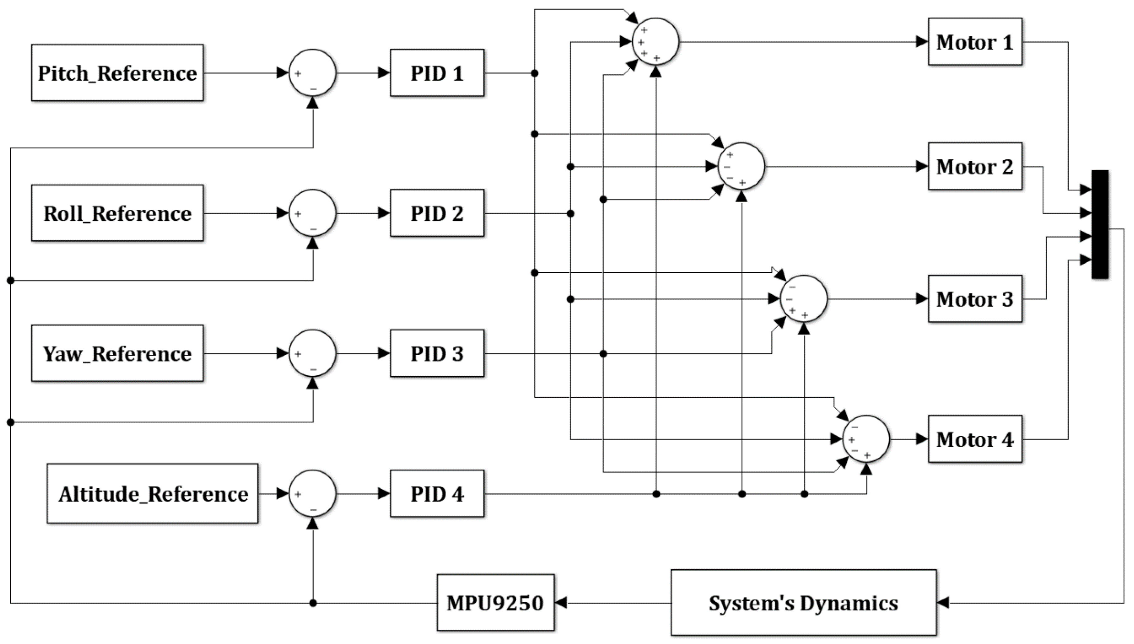
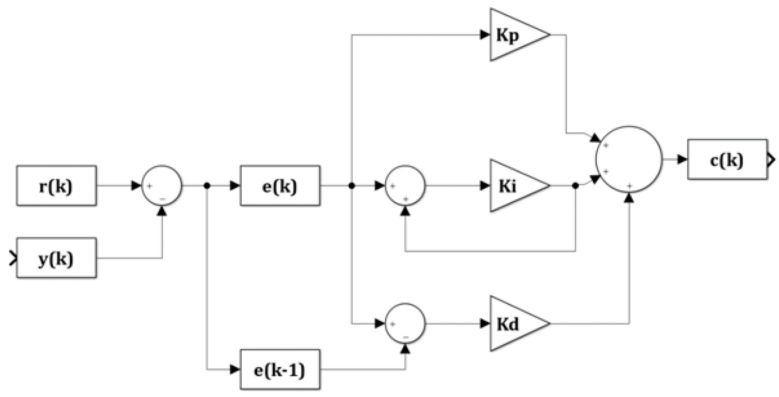
Figure 1 illustrates the block diagram of the control strategy chosen for this quadrotor, with the PID blocks detailed in
Figure 2. The proposed feedback control requires feedback signals and disturbance identification. To obtain these signals, a sensor with 9 degrees of freedom, consisting of an accelerometer, a gyroscope, and a magnetometer is used. Signals from this sensor must be processed because they suffer from noise disturbance and other drawbacks. For example the gyroscope has a flowing bias. This inconvenient is mitigated by the estimator. Both data filtering and estimating the orientation of the aerial vehicle are realized with the quaternion representation of the estimator (27,28). The nonlinear dynamic model (55) is used as predictor in the control structure.
In
Figure 2 the signals are denoted as follows: r(k) is the reference signal at current iteration k; c(k) represents the control signal at this current iteration k; y(k) is the output of the system, measured by sensors at iteration k; e(k) is the error signal at iteration k; K
p, K
i, and K
d represent the proportionality, integration, and derivation constant, respectively. Regarding the angular velocities of the motors, it is necessary to ensure that they behave according to the control signals received from the angular position and altitude controllers. In view of the microcontroller’s processing capacity and the relatively large dimensions of the program used to obtain the inclination angles and the control law previously determined, four electronic speed control modules (ESCs) will be used to control the angular velocities of the motors.
The verification of the designed controllers was first performed through a numerical simulation. The non-linear model from Equation (55) was used to carry out all simulations. Several simulation scenarios were adjusted in order to set the simulation closer to reality. Furthermore, some restrictions related to the actuators were applied based on real data measurements. The delay of the actuators was implemented because of the use of the electronic speed controller (ESC). Moreover, sensor noise was implemented to the measured feedback signals. The evaluation of the designed controller was done both in disturbance free, constant disturbance, and real disturbance conditions. In each case the quadrotor has to follow the same trajectory, including takes off, flying from point A to B, and rotation around the Z axis. As quality indicators chosen to discuss the efficiency of the proposed algorithm are the steady state position error, overshoot, and settling time. In all cases the proposed simple control structure exhibit very similar behavior to advanced, expensive solutions.
3. Results
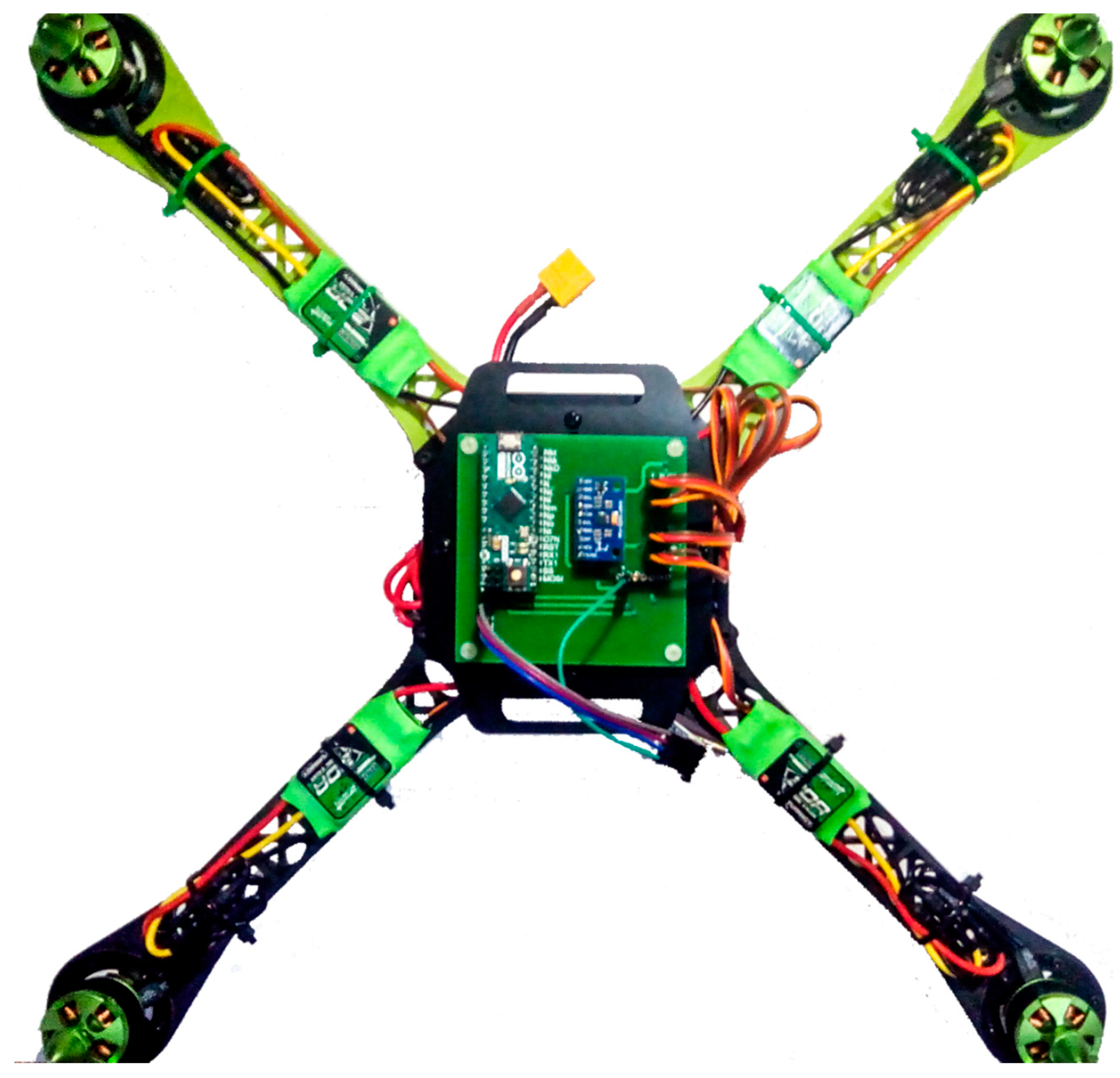
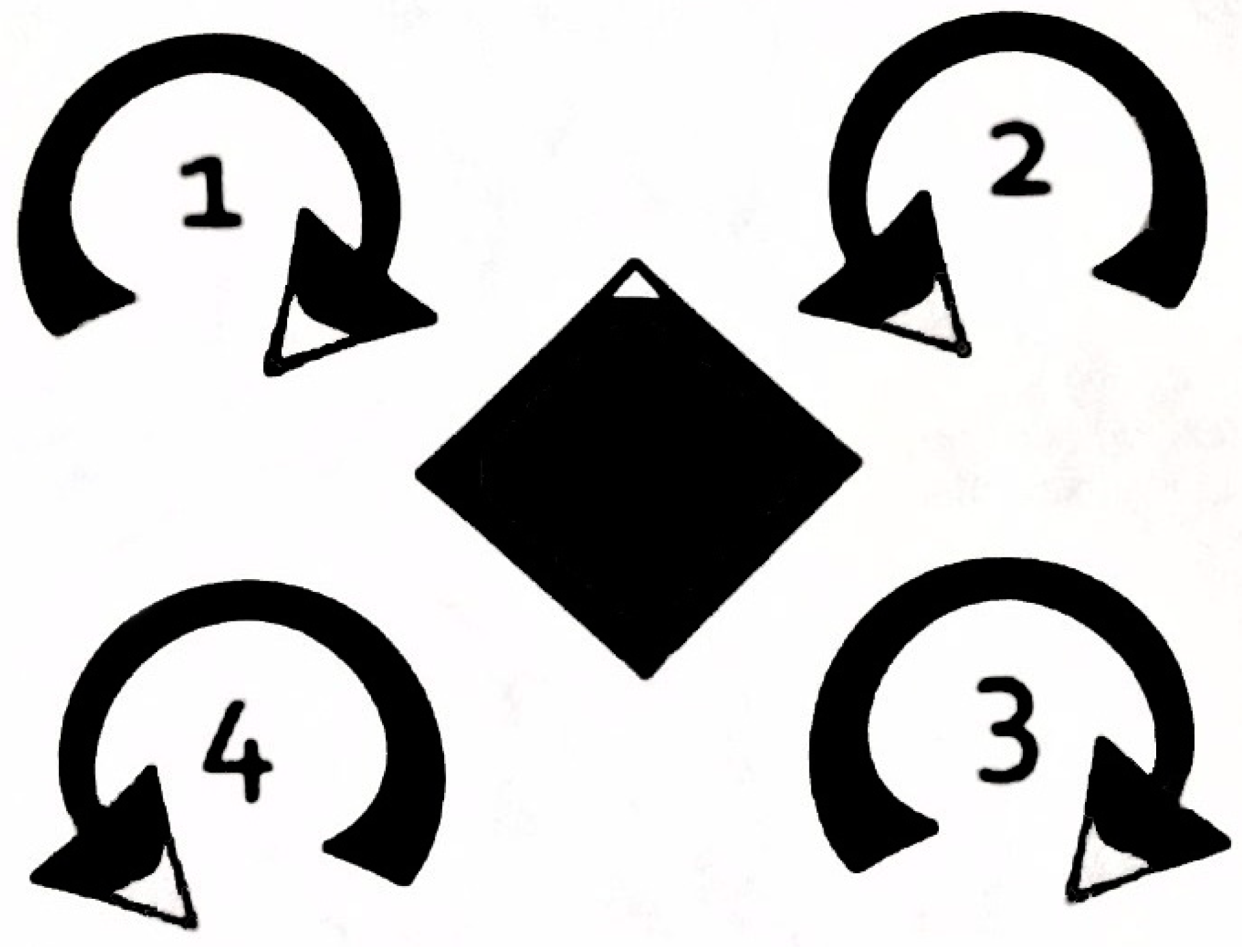
Figure 3 presents the resulted low-cost quadrotor UAV. It has four motors controlled by electronic speed controllers rotating as described in
Figure 4. Each motor is mounted on a plastic arm, which in turn is attached to the carbon fiber central structure. All pieces were chosen so that the assembly has the lowest weight and, at the same time, to maintain the condition of the center of gravity described in the previous section.
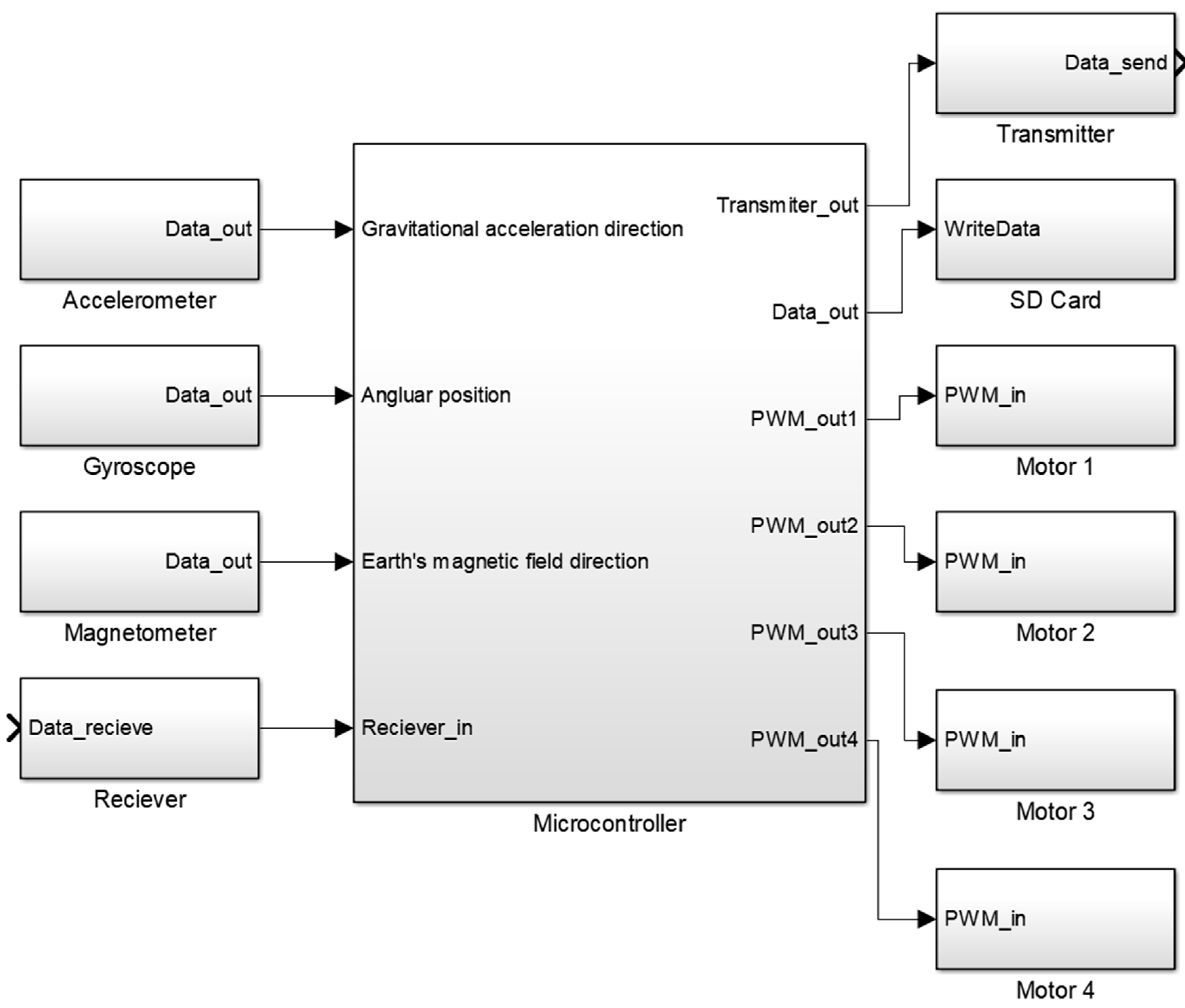
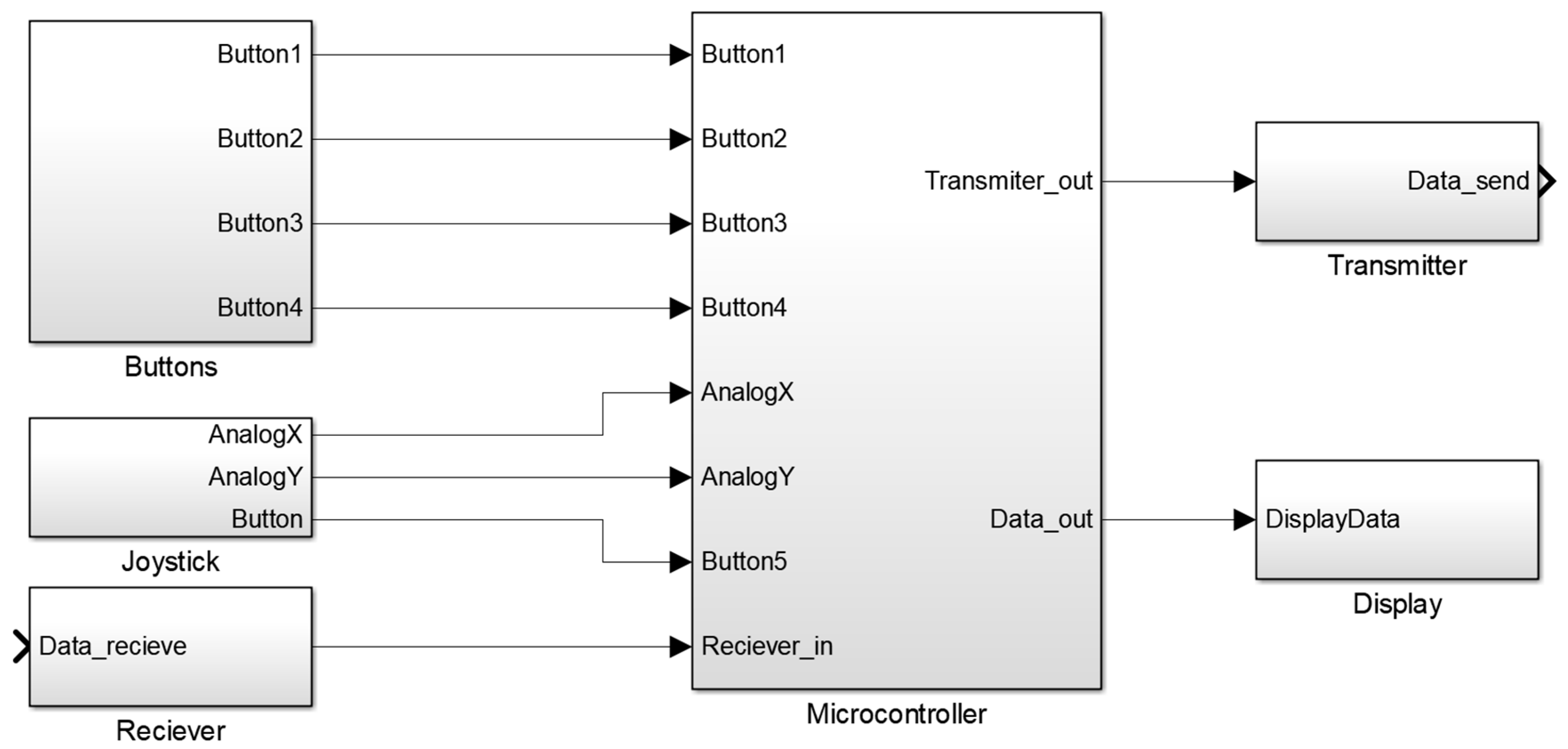
In each step of the design, the aim was to understand the functionality of each component of the system and to describe the relationships between them using block diagrams. In this regard
Figure 5 and
Figure 6 detail the block diagrams of each subsystem, highlighting the type of data provided by/for each element.
In accordance with these block schemes and the dimensions imposed by the mechanical elements, a series of electrical components were chosen. These have been selected so that they can achieve the specifications of the desired control, allow flexibility in resolving errors and have low cost. Also, from the point of view of the processing capacity and the number of input and output signals, respectively, a microcontroller was chosen that satisfies these conditions.
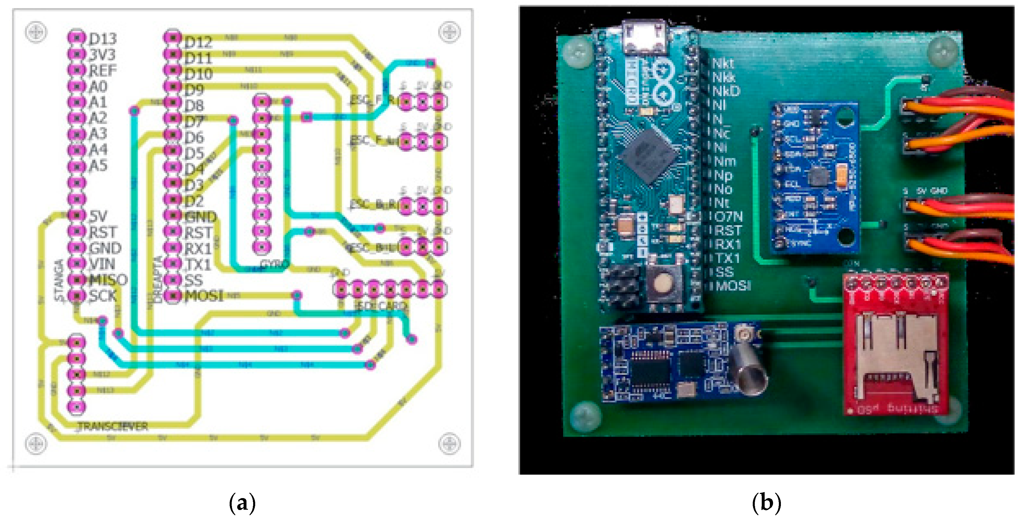
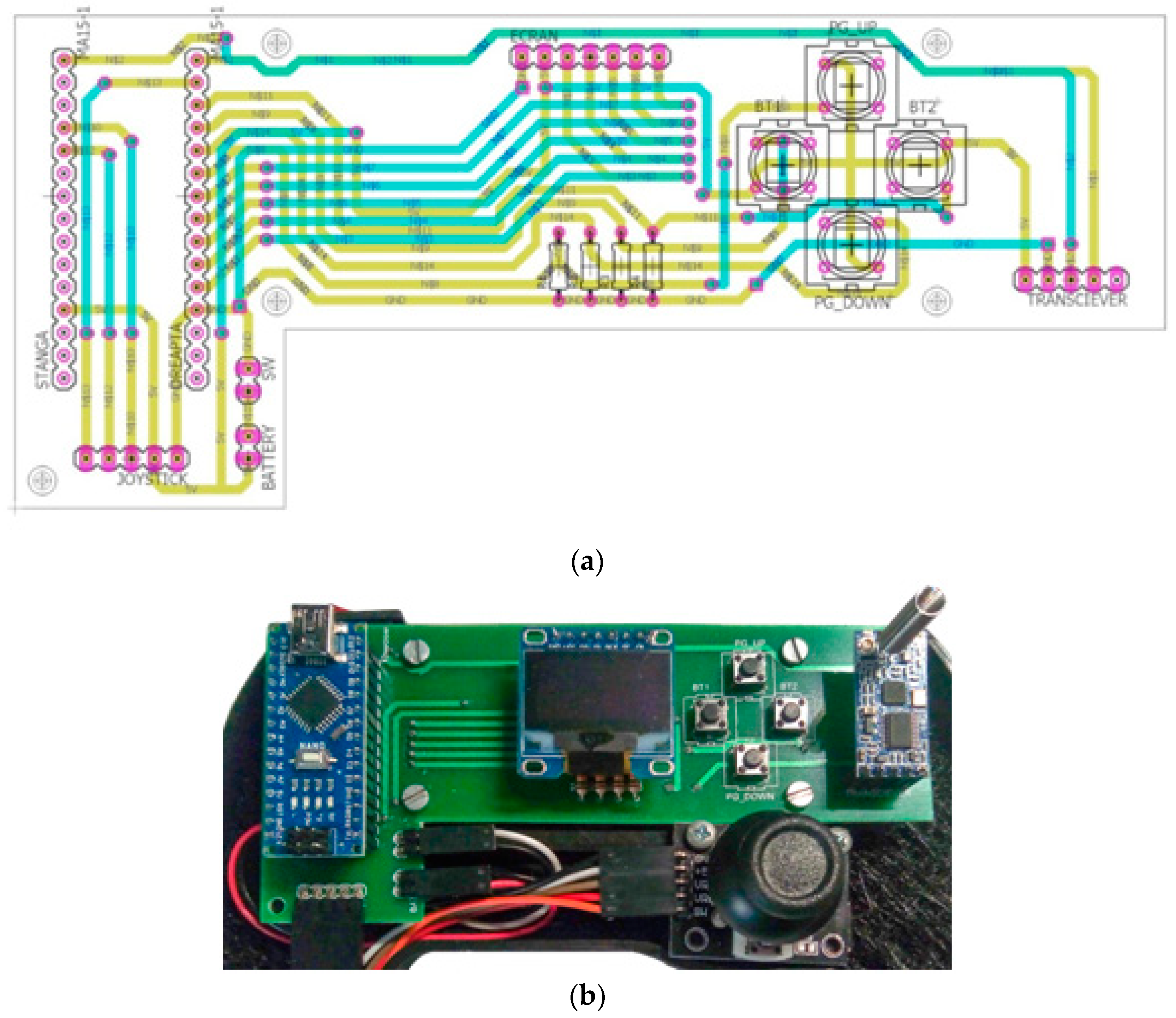
The wiring diagram and the implemented UAV system are presented in
Figure 7. The corresponding remote controller schemes are in
Figure 8, where (a) represents the wiring diagram designed in Eagle, while (b) is the implemented circuit.
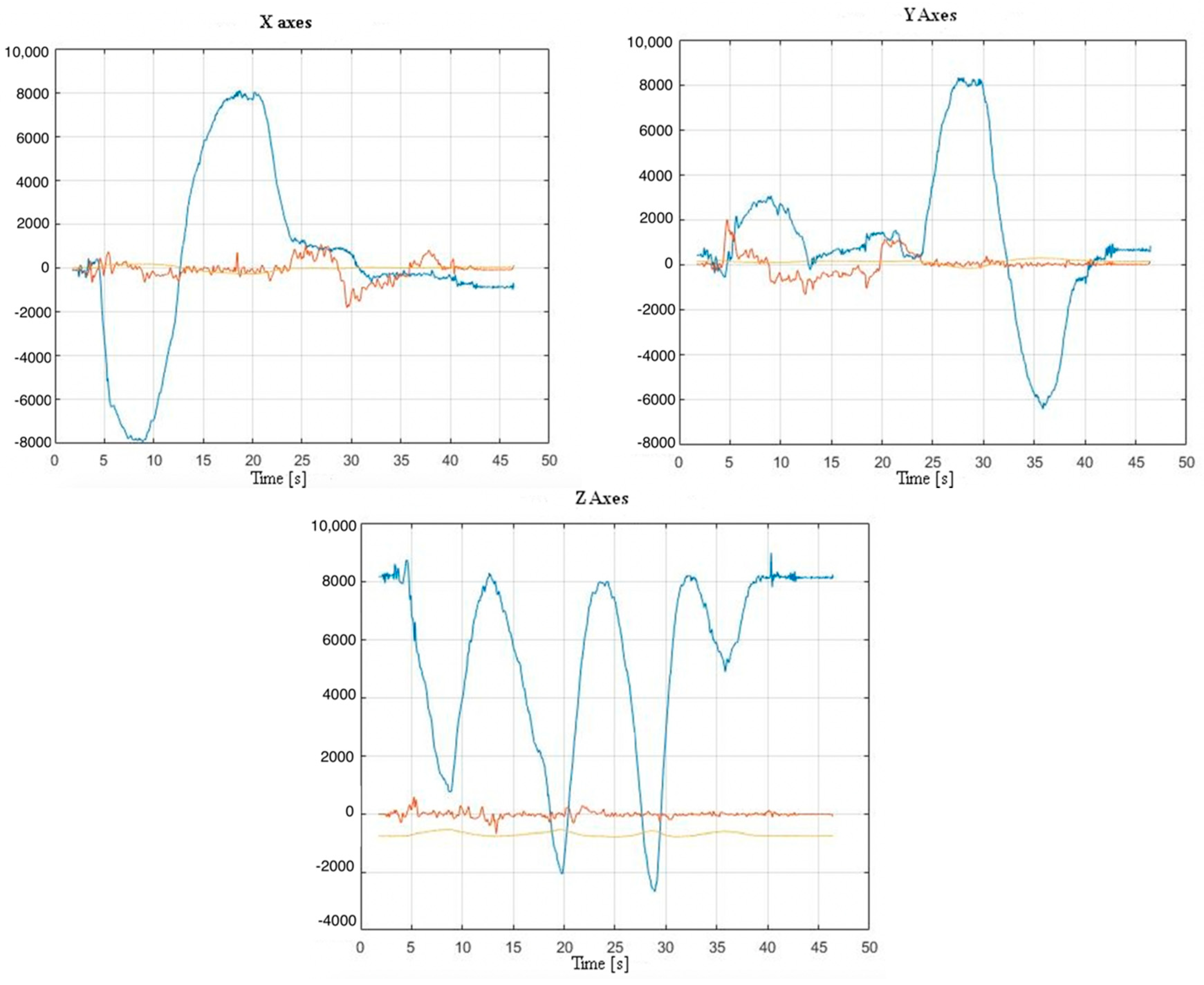
Measurements were realized without using the developed estimator.
Figure 9 presents the raw results of the gyroscope, accelerometer and magnetometer for a linear movement. It can be concluded that in the case of noisy signals, such an approach is not usable in a feedback control structure. It is obvious the necessity of the estimator.
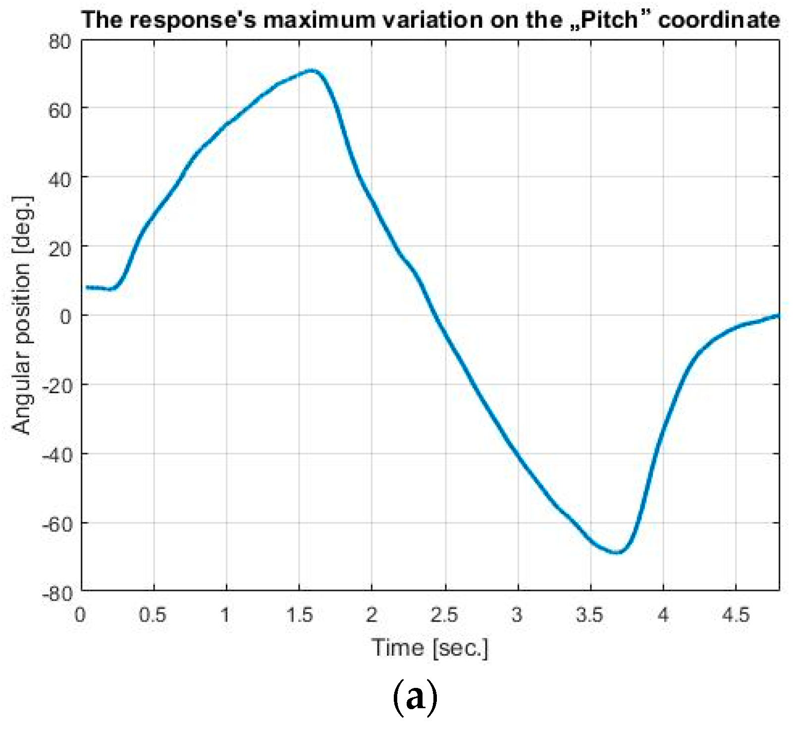
The quaternion-based estimation algorithm described in the previous section was implemented on the microcontroller. In order to test the obtained system, a reference sequence of the form: 0, maximum value to the right, maximum value to the left was applied. The obtained results are plotted in
Figure 10.
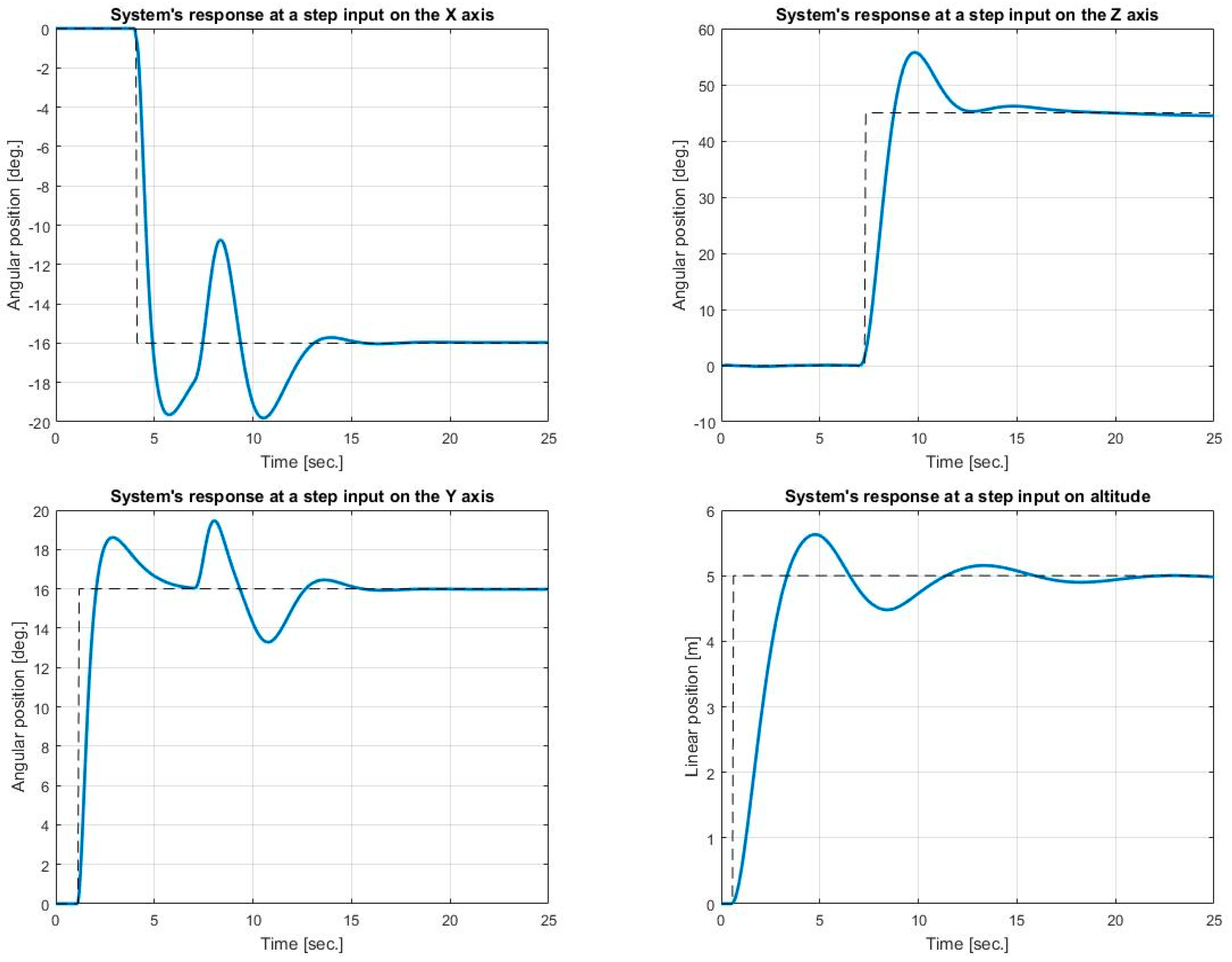
The designed nonlinear model was tested, obtaining the results from
Figure 11.
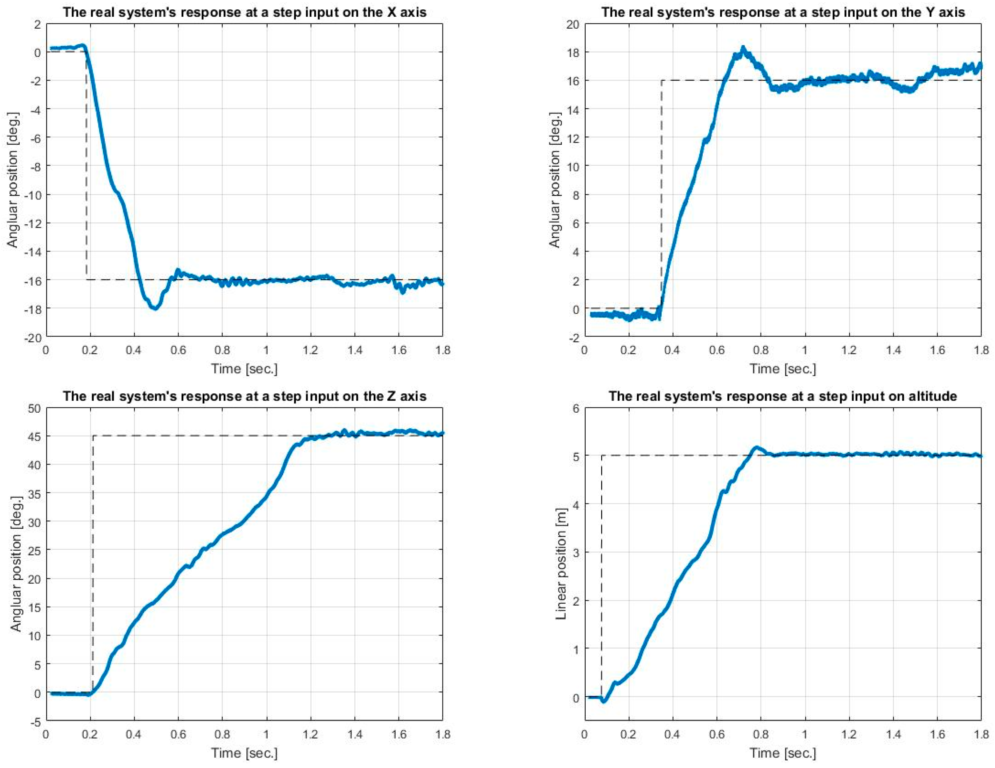
The designed control algorithms were also implemented on the microcontroller. The obtained results in the worst-case scenario, windy conditions, are plotted on
Figure 12, presenting the response of the closed loop system to a step reference on each of the four directions of movement.
The performance was measured for different operation scenarios, including different step inputs on each axis, wind-free and windy conditions. The results for one of the “classical” scenarios—16° step input for angular position on X and Y axis and 45° on Z axis, 5 m altitude, with relatively high wind speed—are presented in
Table 1, highlighting good performances. All these results are comparable with the results of advanced control algorithms in [
25,
26,
27,
28,
29,
30,
31,
32,
33,
34,
35,
36], without needing expensive hardware equipment. In [
26], where the studied quadrotor is similar with our prototype, a LQR controller is used for altitude and a PD controller for position, resulting in a settling time for a step input between 2 and 3.7 s and overshoot 13–20%. Using a backstepping controller combined with the PD, the settling time varies between 2.10 and 3.70 s and the overshoot between 12 and 14%. The LQR controller used both for altitude and position, the settling time are 2.7–3.35 s, while the overshoot is 19–25%. The combination of the backstepping controller with LQR leads to values varying between 2.7–3.3 s, overshoot 15–25%. In our experiments the overshot does not exceed 13.75% neither in worst case and the largest settling time is 1.2 s. The model identification adaptive control (MIAC) used in [
28] leads to settling time between 0.8 and 1.4 s, while with the Model Reference Adaptive Control (MRAC) from the same study, the achieved settling time is of 0.75–2 s, very close to our values. The main advantages of these two (MIAC and MRAC) controllers are the overshoot cancellation, but the cost is the control effort. Analyzing the active disturbance rejection controller designed in [
11], the presented settling times are 0.85–1.5 s for a 20° step input, overshoot is 7–25%, comparable with our results. The advantage of the high-order sliding mode-based fixed-time active disturbance rejection control from [
11] is that it tracks the unknown disturbances in about 3 s.
Comparing our results with the results of the bioinspired controller from [
10], the present results are still competitive. Moreover, imposing different settling time and overshoot in the design stage, it is possible to set a different transient response. Reducing the overshot will increase the settling time and vice versa. Obviously, designing an advanced controller could increase the performances, but the idea of present work was to analyze the most simple algorithm, a PID controller.


