Solitary Wave Solutions of the Generalized Rosenau-KdV-RLW Equation

Abstract

This paper investigates the solitary wave solutions of the generalized Rosenau–Korteweg-de Vries-regularized-long wave equation. This model is obtained by coupling the Rosenau–Korteweg-de Vries and Rosenau-regularized-long wave equations. The solution of the equation is approximated by a local meshless technique called radial basis function (RBF) and the finite-difference (FD) method. The association of the two techniques leads to a meshless algorithm that does not requires the linearization of the nonlinear terms. First, the partial differential equation is transformed into a system of ordinary differential equations (ODEs) using radial kernels. Then, the ODE system is solved by means of an ODE solver of higher-order. It is shown that the proposed method is stable. In order to illustrate the validity and the efficiency of the technique, five problems are tested and the results compared with those provided by other schemes.

1. Introduction

Nonlinear waves are important phenomena in scientific research. Due to that reason, a number of models have been proposed to describe their behavior. Indeed, we find a variety of mathematical descriptions of wave dynamics, such as the Rosenau, regularized-long wave (RLW), and Korteweg-de Vries (KdV) equations [1,2,3,4,5,6,7,8]. The KdV equation has been applied in the description of dynamical effects such as longitudinal astigmatic, ion sound, and magnetic fluid waves [4,5,6,7,8,9]. The convergence properties, existence and the regularity of solutions of KdV-type equation have been discussed in [10,11,12].

Kaya and Aassila calculated the explicit solutions of the KdV equation with an initial condition by using the Adomian decomposition method [13]. Özer and Kutluay applied an analytical–numerical method to the KdV equation [14]. The RLW equation was developed by Peregrine, as an alternative to the classical KdV formulation in order to investigate the behavior of the solution  [15,16]. Benjamin et al. proved the existence and uniqueness of the solution of the RLW model and determined its exact expression subject to restrictions in the initial and boundary conditions  [2]. The RLW is also adopted in the modeling of long waves with small amplitudes on the water surface [17]. A noteworthy feature of the RLW problem is that the collision between two solitary waves results either in sinusoidal solutions, or in secondary solitary waves [18]. Since the KdV cannot describe wave–all and wave–wave interactions, another model, known as the Rosenau equation, was proposed by Rosenau to describe the dynamics behavior of dense discrete systems [7]. Zuo studied the solitary wave and periodic solutions for the Rosenau-KdV model [6]. Barreto et al. discussed the existence of solutions of the Rosenau formulation with the plus sign in the advection-like term in moving domains by means of the Galerkin, multiplier, and energy estimate techniques [3].

Hereafter, we propose a numerical method for the initial value problem of the general Rosenau-KdV-RLW equation [19,20,21,22,23,24],

$$u_t+\alpha u_x+\beta {\left(u^p\right)}_x+\gamma u_{xxx}-\mu u_{xxt}+\delta u_{xxxxt}=0,$$

(1)

with the initial condition

$$u(x,0)=f\left(x\right)$$

(2)

and boundary conditions

$$u(a,t)=u(b,t)=0,u_x(a,t)=u_x(b,t)=0,u(a,t)=u(b,t)=0,u_{xx}(a,t)=u_{xx}(b,t)=0,$$

(3)

where $u=u(x,t),$ is a real-valued function, the real constants $\alpha ,\beta ,\gamma$ and $\mu$ are non-negative, $p\ge 2$ is a positive integer, and $f\left(x\right)$ is a given smooth function.

Lemma 1.

(See [25].) The following conservative properties for the initial value problem (1) hold

$$Q\left(t\right)={\int }_a^{b}u(x,t)dx={\int }_a^{b}u(x,0)\mathrm{d}x=Q\left(0\right)$$

(4)

and

$$E\left(t\right)={\int }_a^b(u^2+c{u}_x^2+u_{xx}^2)\mathrm{d}x={\left|\right|u\left|\right|}_{L^2}^2+c\left|\right|u_x{\left|\right|}_{L^2}^2+c\left|\right|u_{xx}{\left|\right|}_{L^2}^2=E\left(0\right),$$

(5)

where $Q\left(0\right)$ and $E\left(0\right)$ are constants depending on the initial conditions.

When $-a\gg 0$ and $b\gg 0$, the initial boundary value problem (1)–(3) is consistent and, the boundary condition (3) is reasonable [26]. Some particular cases of Equation (1) occur:

• if $\alpha =0,\beta =0.5,\gamma =1,\mu =0,\delta =0$ and $p=2$, then expression (1) is the KdV equation [14,27,28,29],

  $$u_t+u{u}_x+u_{xxx}=0;$$
• if $\alpha =1,\beta =0.5,\gamma =0,\mu =0,\delta =1$ and $p=2$, then expression (1) is the Rosenau equation [30,31,32],

  $$u_t+\alpha u_x+u{u}_x+u_{xxxt}=0;$$
• if $\alpha =1,\beta =0.5,\mu =1,\gamma =0,\delta =0$ and $p=2$, then expression (1) becomes the RLW equation [33]

  $$u_t+u_x+u{u}_x-u_{xxt}=0;$$
• if $\alpha =1,\beta =0.5,\gamma =1,\mu =0,\delta =1$ and $p=2$, then expression (1) is the Rosenau-KdV equation [6,34,35]

  $$u_t+u_x+u{u}_x+u_{xxx}+u_{xxxxt}=0;$$
• if $\alpha =1,\beta =1,\gamma =0,\mu =1,$ and $\delta =1,$ then expression (1) is the generalized Rosenau-RLW model [26]

  $$u_t+u_x+{\left(u^p\right)}_x-u_{xxt}+u_{xxxxt}=0;$$
• if $p=2$, $p=3$ or $p\ge 4,$ then expression (1) represents the classical, modified, and general Rosenau-RLW equations, respectively.

In recent years, various analytical and numerical methods have been used to approximate the solution of the initial boundary value problem (1)–(3). Razborova et al. presented a theoretical approach based on the Ansatz method for the Rosenau-KdV-RLW equation [9]. Later, Razborova et al. used a semi-inverse Variational Principle to retrieve a single solitary wave solution [22]. Additionally, Razborova et al. and Sanchez et al. discussed the solutions of the perturbed Rosenau-KdV-RLW equation [23,24]. Wongsaijai et al. constructed a three-level weighted average implicit finite difference (FD) technique [19]. Pan et al. presented a C-N pseudo-compact conservative numerical scheme based on the FD technique [20]. Fernández and Ramos investigated a three-point compact method with fourth-second accuracy [21]. Wang et al. and Hu and Wang formulated FD schemes with linear three-level [31] and high-accuracy conservative [33] characteristics, respectively. Wongsaijai et al. proposed a compact FD technique [26] and Pan et al. developed a linear-implicit FD for the usual Rosenau-RLW equation [25,36]. Zheng et al. presented an average linear FD technique [34]. Mittal et al. implemented a numerical method based on the collocation of quintic B-splines over finite elements [37]. Hu et al. considered a second-order conservative FD scheme [38]. Ari et al. adopted a meshless kernel-based approach of lines  [39]. Foroutan et al. developed a modified Chebyshev rational approximation [40]. Wang et al. advanced a three-level linear conservative FD [41], while Wongsaijai et al. came with a mass-preserving scheme, namely, a nonlinear algorithm based on a modification of the FD [42].

In this paper, we use the local meshless radial basis function (RBF) for solving the general Rosenau-KdV and the Rosenau-RLW models. Section 2 formulates and discusses the local meshless RBF based on the finite difference (RBF-FD) technique for discretizing Equation (1). Section 3 provides five numerical examples and compares the results with those of other schemes proposed in the literature. Finally, Section 4 presents the concluding remarks.

2. The RBF-FD Collocation Method

A mesh-free (or meshless) method adopts an algebraic system of equations for the complete domain without requiring a pre-defined mesh discretization of the domain and its boundary [43,44]. Mesh-free techniques are used to approximate scattered data, since generating meshes is one of the most laborious tasks of mesh-based numerical processes. Indeed, a mesh-free technique provides a low-cost alternative to schemes involving finite volume, finite difference, finite element, multivariate splines, and wavelets, all requiring node connectivity. Meshless techniques eliminate the mesh generation step and a collection of scattered data can be used. The RBF is one of the most widely used meshless techniques and reveals good performance in case of multidimensional scattered data interpolation [43,44].

Given a set of scattered node data $X_C=\{x_1,\dots ,x_N\}\subseteq {\mathrm{R}}^n$ and the corresponding function values $u_i=u\left(x_i\right),i=1,2,\dots ,N$, the RBF interpolant is represented in the form

$$u\left(x\right)\simeq S\left(x\right)=\sum _{j=1}^N{\alpha }_j{\varphi }_j(x,c),$$

(6)

where ${\left\{{\alpha }_j\right\}}_{j=1}^N$ are unknown coefficients, ${\varphi }_j(x,c)=\varphi (\parallel x-x_j{\parallel }_2,c),$$j=1,\dots ,N,$ are RBF with shape parameter c, and the operation ${\parallel ·\parallel }_2$ represents the Euclidean norm [44,45]. Some popular choices of RBF include the linear, Cubic, Multiquadric (MQ), Gaussian (GA), and thin-plate spline (TPS) versions with dependence r, $r^3$, $\sqrt{c^2+r^2}$, $exp(-c{r}^2)$, and $r^{4}ln\left(r\right)$, respectively, where $r=\parallel x-x_j{\parallel }_2$. The coefficients ${\left\{{\alpha }_j\right\}}_{j=1}^N$ of Equation (6) are computed by imposing interpolation conditions $S\left(x_i\right)=u_i$, $i=1,\dots ,N.$ The relation (6) can be written in the following matrix form

$$A_{\varphi }\alpha =f,$$

(7)

where  

$$\begin{array}{c}\hfill \alpha =\left[\begin{array}{c}{\alpha }_1\\ {\alpha }_2\\ ⋮\\ {\alpha }_N\end{array}\right],f=\left[\begin{array}{c}{f}_1\\ f_2\\ ⋮\\ f_N\end{array}\right],A_{\varphi ,ij}={\varphi }_j\left(x_i\right),i,j=1,\dots ,N.\end{array}$$

The non-singularity of the associated linear system was proven in [46]. The main pros of the RBF collocation method when solving PDEs are its simplicity, easy application to different PDEs, and efficiency for solving problems involving complex domains. On the other hand, the major con of this method is related to the problem of full matrices. These matrices are strongly sensitive to the shape parameter c selected in the RBF and, therefore, they become difficult to solve in problems where we have too many unknowns. This problem arises from the fact that using the RBF interpolation increases the condition numbers of the related matrices for a large number of nodes. This occurs particularly when one selects inadequate data centers and uses basic functions that are infinitely smooth, such as the MQ, with extreme values of the shape parameter c [45].

The notation of local differentiation is popular in the RBF literature, particularly for time-dependent PDEs. The local radial basis function (RBF) generated by finite differences (RBF-FD), raised considerable interest owing to the structure of their differentiation and interpolation matrices [47,48]. It is possible to control the degree of sparsity of the differentiation and interpolation matrices produced by the local RBF. This sparsity can take advantage of parallelism and solve large problems [49,50]. The local RBFs have also been employed to reduce the model order. In some situations, researchers have found that the local RBF technique can produce the same degree of accuracy as the global RBF technique with a smaller mesh size [49,50,51,52,53]. Although small mesh sizes result in smaller ODE systems, the overall accuracy is maintained. Interested readers can find examples of the application of local RBFs to problems in the geosciences in [54,55]. Garshasbi et al. used the RBF collocation method for approximating the shallow water model named the Camassa–Holm equation [56]. Uddin connected the RBF to the pseudo-spectral method, known as RBF-PS method to approximate the equal width equation [57]. Nikan et al. solved numerically the nonlinear KdV-Benjamin-Bona-Mahony-Burgers (KdV-BBM-B) with the help of the RBF-PS [58]. Dehghan and Shafieeabyaneh addressed the RLW and extended Fisher-Kolmogorov (EFK) equations using local meshless RBF-FD [59]. Ebrahimijahan and Dehghan proposed a numerical technique for solving the nonlinear generalized BBBM-B and RLW equations based on the integrated RBF [60]. Rashidinia et al. implemented the local RBF-FD meshless method for generalized Korteweg-de Vries-Burgers [61] and Kawahara [62] equations.

Let us consider that $I_i=\{x_{i_1},x_{i_2},\dots ,x_{i_{n_i}}\}$ is a stencil of $x_i$. In the local RBF-FD collocation method, the linear differential operator $\mathcal{L}$ at every point can be approximated only the stencil instead of applying the complete number of point, i.e.,

$$\mathcal{L}u\left(x_i\right)=\sum _{j=1}^{n_i}{w}_{j}u\left(x_{i_j}\right),$$

(8)

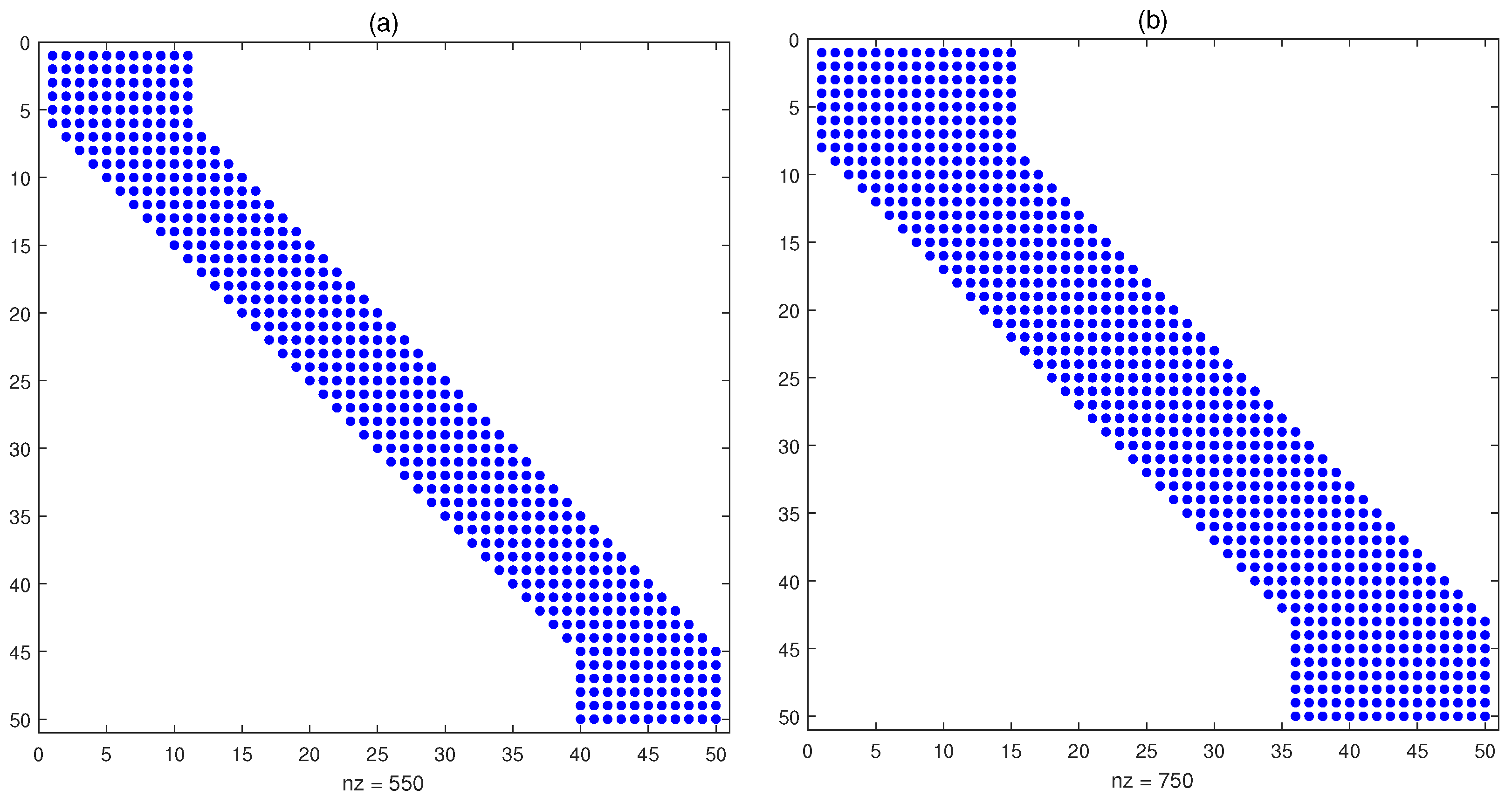
where $x_i=x_{i_1}$ is the center point of stencil $I_i$. Figure 1 gives an example of a domain with 9 grid points and a stencil size of $n_i=4$. At the point $x_3$, the $n_i-1=3$ nearest neighbors are used in the computation. Figure 2 shows the sparsity patterns for $N=50$ for two stencil sizes $n_i=11$ and $n_i=15$.

Figure 1. Illustration of one-dimensional case of stencil.

Figure 2. Sparsity patterns for $N=50$ and two stencil sizes $n_i=11$ (a) and $n_i=15$ (b).

By deriving the RBF expansion of $u\left(x\right)$ in Equation (8), the weighted differences of stencil node can be obtained from the system as:

$$A_{\varphi }w=l,$$

(9)

where

$$\begin{array}{c}\hfill w=\left[\begin{array}{c}{w}_1\\ w_2\\ ⋮\\ w_{n_i}\end{array}\right],l=\left[\begin{array}{c}\mathcal{L}{\varphi }_{i_1}\left(x\right){|}_{x=x_i}\\ \mathcal{L}{\varphi }_{i_2}\left(x\right){|}_{x=x_i}\\ ⋮\\ \mathcal{L}{\varphi }_{i_{n_i}}\left(x\right){|}_{x=x_i}\end{array}\right],A_{\varphi ,ij}={\varphi }_{i_i}\left(x_{i_j}\right),i,j=1,\dots ,n_i.\end{array}$$

(10)

Indeed, it is necessary to solve a small-sized linear system with a conditionally positive definite coefficient matrix in each stencil. The weighted differences of the stencil nodes $w_1,w_2,\dots ,w_{n_i}$ can be determined from the above system.

The first, second and third order derivatives can be approximated with the help of the function values at a set of $n_i$ nodes (including $x_i$) in the stencil of $x_i$. That is, we can write

$$\begin{array}{c}\frac{\partial u^k\left(x\right)}{\partial x}{|}_{x=x_i}=\sum _{j=1}^{n_i}{w}_{i,j}^{x,1}{u}^k\left(x_j^i\right)={\mathbf{W}}_x\mathbf{u},\hfill \end{array}$$

(11)

$$\begin{array}{c}\frac{{\partial }^2{u}^k\left(x\right)}{\partial x^2}{|}_{x=x_i}=\sum _{j=1}^{n_i}{w}_{i,j}^{x,2}{u}^k\left(x_j^i\right)={\mathbf{W}}_{xx}\mathbf{u},\hfill \end{array}$$

(12)

$$\begin{array}{c}\frac{{\partial }^3{u}^k\left(x\right)}{\partial x^3}{|}_{x=x_i}=\sum _{j=1}^{n_i}{w}_{i,j}^{x,3}{u}^k\left(x_j^i\right)={\mathbf{W}}_{xxx}\mathbf{u},\hfill \end{array}$$

(13)

where $w_{i,j}^{x,l}$ represents the weighted differences of stencil node for the order derivatives $l=\{1,2,3\}.$

We can obtain the following semi-discrete system by considering the notations above as

$${\mathbf{u}}^{{}^{\prime }}+\alpha {\mathbf{W}}_x\mathbf{u}+\beta {\mathbf{W}}_x\left({\mathbf{u}}^p\right)-\mu {\mathbf{W}}_{xx}{\mathbf{u}}^{{}^{\prime }}+\gamma {\mathbf{W}}_{xxx}+\delta {\mathbf{W}}_{xxxx}{\mathbf{u}}^{{}^{\prime }}=0.$$

(14)

The above equation can be represented as

$$(\mathbf{I}-\mu {\mathbf{W}}_{xx}+\delta {\mathbf{W}}_{xxxx}){\mathbf{u}}^{{}^{\prime }}=-\alpha {\mathbf{W}}_x\mathbf{u}-\beta {\mathbf{W}}_x\left({\mathbf{u}}^p\right)-\gamma {\mathbf{W}}_{xxx}\mathbf{u}.$$

(15)

We must note that the matrices $\mathbf{A}=-\alpha {\mathbf{W}}_x-\beta {\mathbf{W}}_x-\gamma {\mathbf{W}}_{xxx}$ and $\mathbf{B}=\mathbf{I}-\mu {\mathbf{W}}_{xx}+\delta {\mathbf{W}}_{xxxx}$ are time-independent. We conclude that

$${\mathbf{u}}^{{}^{\prime }}=\mathbf{W}\mathbf{u},$$

(16)

where $\mathbf{W}={\mathbf{B}}^{-1}(-\alpha {\mathbf{W}}_x-\beta {\mathbf{W}}_x\left({\mathbf{u}}^{p-1}\right)-\gamma {\mathbf{W}}_{xxx})$. Equation (16) is of the form

$${\mathbf{u}}^{{}^{\prime }}=F\left(\mathbf{u}\right).$$

(17)

Equation (17) is an ODE with respect to $\mathbf{u}$ and it can be solved by means of an ODE solver in MATLAB such as ode113 or ode45. Let $\tau =T/M$ and $t_n=n\tau ,$ for $n=0,1,\cdots ,M,$ so that the mesh $\{t_n:n=0,1,\cdots ,M\}$ is uniform. The initial solution $u_0$ is the starting vector. The package ode45 is an explicit Runge-Kutta of order 4(5) formula of the Dormand–Prince pairs [63]. The ode45 is a one-step solver that computes $u_{t_n}$ given the solution at the preceding time point $u_{t_{n-1}}$. On the other hand, the ode113 is a variable-order Predict–Evaluate–Correct–Evaluate solver of the Adams–Bashforth–Moulton type [64]. This solver might be more efficient than the ode45 for close tolerances and, in particular, when the ODE file function is particularly expensive to evaluate. A multi-step solver, such as the ode113, needs the solutions corresponding to more than one preceding time point for calculating the current solution. Hereafter, we calculate the differentiation matrices, expressed by ${\mathbf{W}}_x$, ${\mathbf{W}}_{xx}$ and ${\mathbf{W}}_{xx}$, only one time outside the time-stepping operation. Additionally, merely matrix-vector multiplications are required within the time-stepping operation.

Stability Analysis

The method of lines represents the idea of using the FD method in the time direction t to solve a coupled system of ODEs. The numerical stability of the method of lines is investigated by a rule of tumb. The method of lines is stable if the eigenvalues of the (linearized) spatial discretization operator, scaled by $\tau$, lie in the stability region of the time-discretization operator [57,65]. One defines the stability region as the portion of a multifaceted plane consisting of eigenvalues which result in the generation of bounded solutions. The coefficient matrix eigenvalues determine the stability of Equation (16) [66]. Hence, we need only to demonstrate that every eigenvalue $Re\left({\lambda }_i\right)$ belonging to the coefficient matrix has a non-positive real term $Re\left({\lambda }_i\right)$, where ${\lambda }_i,i=1,2,\dots ,N,$ represents of the matrix eigenvalues. In other words, for all $i=1,2,\dots ,N,$ we must have $Re\left({\lambda }_i\right)\le 0$ for obtaining stable solutions. The reader is referred to [66] for further details. In order to investigate the stable and unstable eigenvalue ranges of the Rosenau-KdV-RLW model, one must compute the eigenvalues belonging to the matrix $\mathbf{W}$, which are scaled by $\tau$.

3. Computational Results and Comparisons

This section considers five test problems assessing the effectiveness and accuracy of the proposed method for various values of h, $\tau$ and c. To measure the accuracy of method in comparison with the exact solution, we compute the following error norms:

$$\begin{array}{cc}\hfill & L_{\infty }={\displaystyle \underset{1\le j\le M-1}{max}}|u^{exact}(x_j,T)-u^{}(x_j,T)|,\hfill \\ \hfill & L_2={\left(h\sum _{j=1}^N{(u^{exact}(x_j,T)-u^{}(x_j,T))}^2\right)}^{\frac{1}{2}},\hfill \\ \hfill & RMS={\left(\frac{1}{N}\sum _{j=1}^N{(u^{exact}(x_j,T)-u^{}(x_j,T))}^2\right)}^{\frac{1}{2}},\hfill \end{array}$$

where $u^{}$ and $u^{exact}$ denote the numerical solution and exact solution, respectively. In addition, the invariants of motion are evaluated by

$$\begin{array}{cc}\hfill & Q={\int }_a^{b}u(x,t)\mathrm{d}x=\sum _{i=1}^N{u}_i,\hfill \\ \hfill & E={\int }_a^b(u^2+c{u}_x^2+u_{xx}^2)\mathrm{d}x=\sum _{i=1}^N\left(u_i^2+c{\left(u_x\right)}_i^2+{\left(u_{xx}\right)}_i^2\right).\hfill \end{array}$$

It should be noted that the Gaussian function is used as a basis and the computations were performed in MATLAB R2016a with a computer system having a configuration including Intel(R) Core(TM) i5-2330 CPU 3.60 GHz and 8.00G RAM.

Example 1.

Let us consider the general Rosenau-KdV-RLW model (1) in the case of $\alpha =\mu =\gamma =1$, $\beta =0.5$, $p=2$ and $\delta =0$ in the spatial interval $x\in [-70,100]$. The exact solution is $u(x,t)=k_{11}{\mathrm{sech}}^4\left[k_{12}(x-k_{13}t)\right]$ [38,41], where

$$k_{11}=-\frac{35}{24}+\frac{35}{12}\sqrt{313},k_{12}=\frac{1}{24}\sqrt{-26+2\sqrt{313}},k_{13}=\frac{1}{2}+\frac{\sqrt{313}}{26}·$$

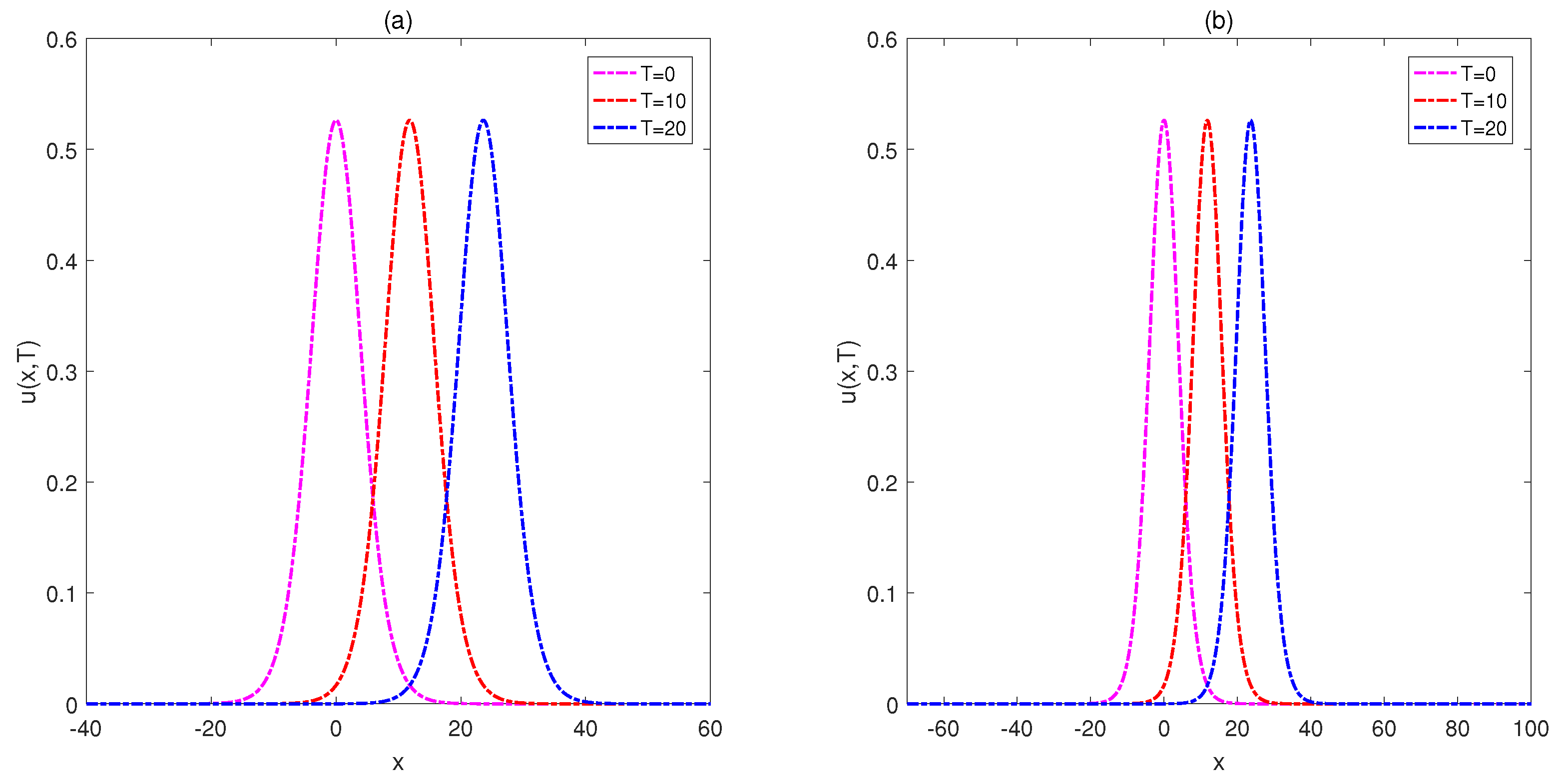
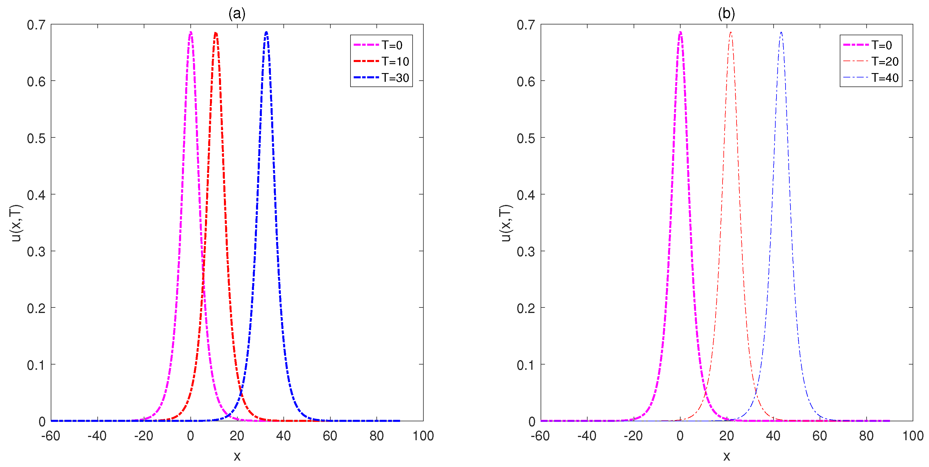
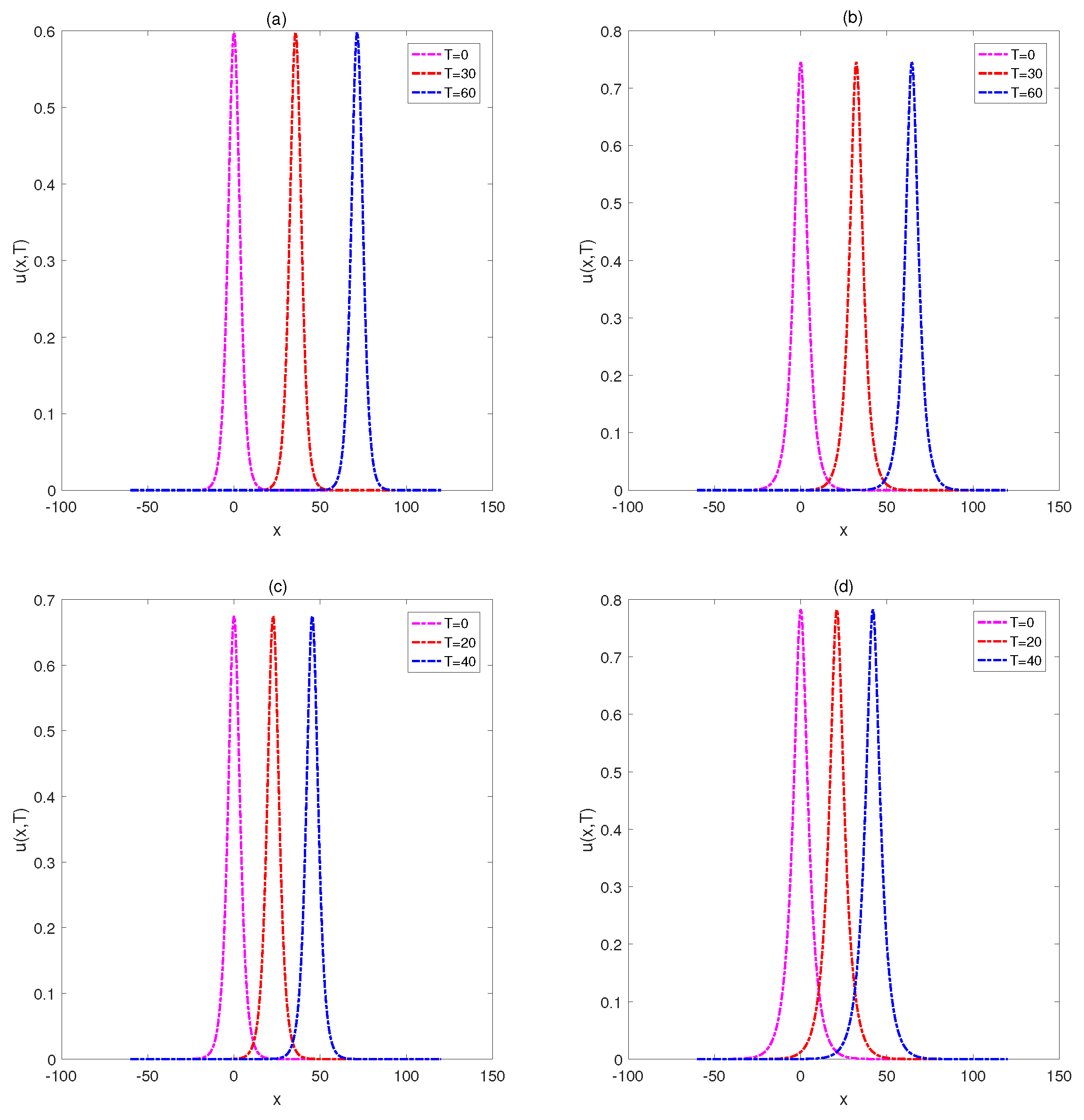
Table 1 lists the approximation errors in terms of $L_{\infty },L_2$ and RMS with $\tau =0.01$ and $n_i=489$. Table 2 compares the obtained results with those provided by the techniques described in [38,41]. It is seen that the errors obtained by the proposed technique are inferior to the others. Figure 3 depicts the motion of the single solitary wave with $h=\tau =0.125$ over the spatial intervals $x\in [-40,60]$ (left) and $x\in [-70,100]$ (right) at final times $T\in \{0,30,40\}.$ We verify that the single solitons move to the right at a constant speed and preserve their amplitude and shape with increasing time as anticipated. 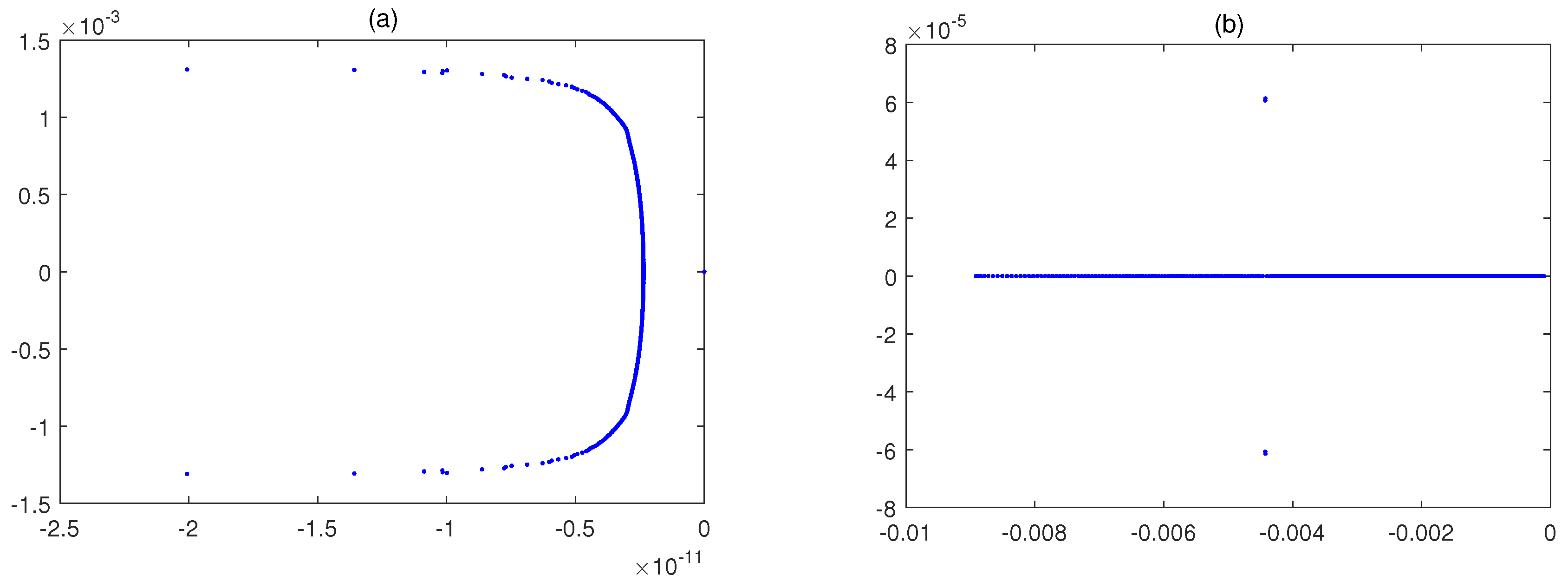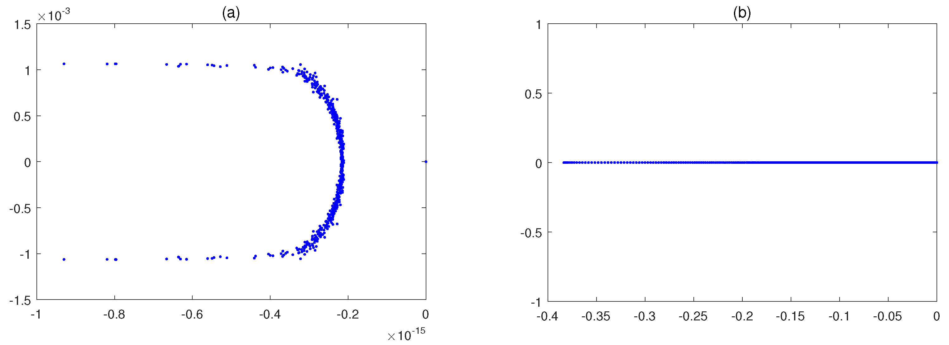Figure 4 represents the absolute errors $L_{\infty }$ at final times $T\in \{0,30,40\}.$ Figure 5 portraits the eigenvalues of the linearized differentiation operator $\mathbf{A}$ and $\mathbf{B}$ (left and right panels, respectively) with $N=100$. We observe that the eigenvalues calculated for $\mathbf{A}$ and $\mathbf{B}$ are zero or have negative values. The eigenvalues belonging to the linearized differentiation operators are real and negative or are complex with a negative real term. Hence, the stability of the proposed system for this case is proven.

Table 1. The $L_{\infty },L_2$ and RMS errors with $\tau =0.01$, $N=100,$$n_i=589$ and $c=1.8$ for Example 1.

Method	T	${\mathit{L}}_{\mathit{\infty }}$	${\mathit{L}}_2$	RMS
RBF-FD	5	$1.7556\times {10}^{-11}$	$4.2037\times {10}^{-11}$	$3.2241\times {10}^{-12}$
RBF-FD	10	$3.4832\times {10}^{-11}$	$8.3499\times {10}^{-11}$	$6.4057\times {10}^{-12}$
RBF-FD	15	$5.1114\times {10}^{-11}$	$1.2388\times {10}^{-10}$	$9.5038\times {10}^{-12}$
RBF-FD	20	$6.6317\times {10}^{-11}$	$1.6066\times {10}^{-10}$	$1.2320\times {10}^{-11}$
RBF-FD	25	$7.9818\times {10}^{-11}$	$4.7209\times {10}^{-10}$	$1.4929\times {10}^{-11}$
RBF-FD	30	$9.2357\times {10}^{-11}$	$2.2541\times {10}^{-10}$	$1.7273\times {10}^{-11}$
RBF-FD	35	$1.0459\times {10}^{-10}$	$2.5348\times {10}^{-10}$	$1.9441\times {10}^{-11}$
RBF-FD	40	$1.1660\times {10}^{-10}$	$2.7268\times {10}^{-10}$	$2.0910\times {10}^{-11}$

Table 2. The $L_{\infty }$ and $L_2$ errors under different mesh steps $h=\tau$ at $T=40$ for Example 1.

	Method	c	N	${\mathit{n}}_{\mathit{i}}$	${\mathit{L}}_{\mathit{\infty }}$	${\mathit{L}}_2$
$h=\tau =0.2$
	RBF-FD	1.65	850	801	$3.8494\times {10}^{-12}$	$9.7017\times {10}^{-12}$
	[41]	−	850	−	$7.8920\times {10}^{-4}$	−
$h=\tau =0.1$
	RBF-FD	3.65	1700	1689	$3.2235\times {10}^{-12}$	$2.8677\times {10}^{-11}$
	[41]	−	1700	−	$1.8771\times {10}^{-4}$	−
	[38]	−	1700	−	$1.1314\times {10}^{-3}$	−
$h=\tau =0.05$
	RBF-FD	5.60	3400	2971	$2.3648\times {10}^{-10}$	$2.9115\times {10}^{-9}$
	[41]	−	3400	−	$2.8359\times {10}^{-4}$	−
	[38]	−	3400	−	$4.6987\times {10}^{-5}$	−

Figure 3. Motion of the single solitary wave with $\tau =h=0.05,$ at various times over the intervals: $x\in [-40,60]$ (a) and $x\in [-70,100]$ (b) for Example 1.

Figure 4. The absolute error $L_{\infty }$ with $\tau =h=0.05,$ at final times $T=30$ (a) and $T=40$ (b) over the interval $x\in [-70,100]$ for Example 1.

Figure 5. The eigenvalues of $\mathbf{A}$ (a) and $\mathbf{B}$ (b) for $N=1000$, $n_i=589$ and $c=1.08$ in Example 1.

Example 2.

Let us consider the general Rosenau-KdV-RLW model (1) in the case of $\alpha =\beta =\mu =\gamma =1$, $p=5$ and $\delta =0$ over the spatial interval $x\in [-60,90]$. The exact solitary wave solution is $u(x,t)=k_{21}\mathrm{sech}\left[k_{22}(x-k_{23}t)\right]$, where [34,41]

$$k_{21}=\sqrt[4]{\frac{4}{15}(-5+\sqrt{34})},k_{22}=\frac{-5+\sqrt{34}}{3},k_{23}=\frac{5+\sqrt{34}}{10}·$$

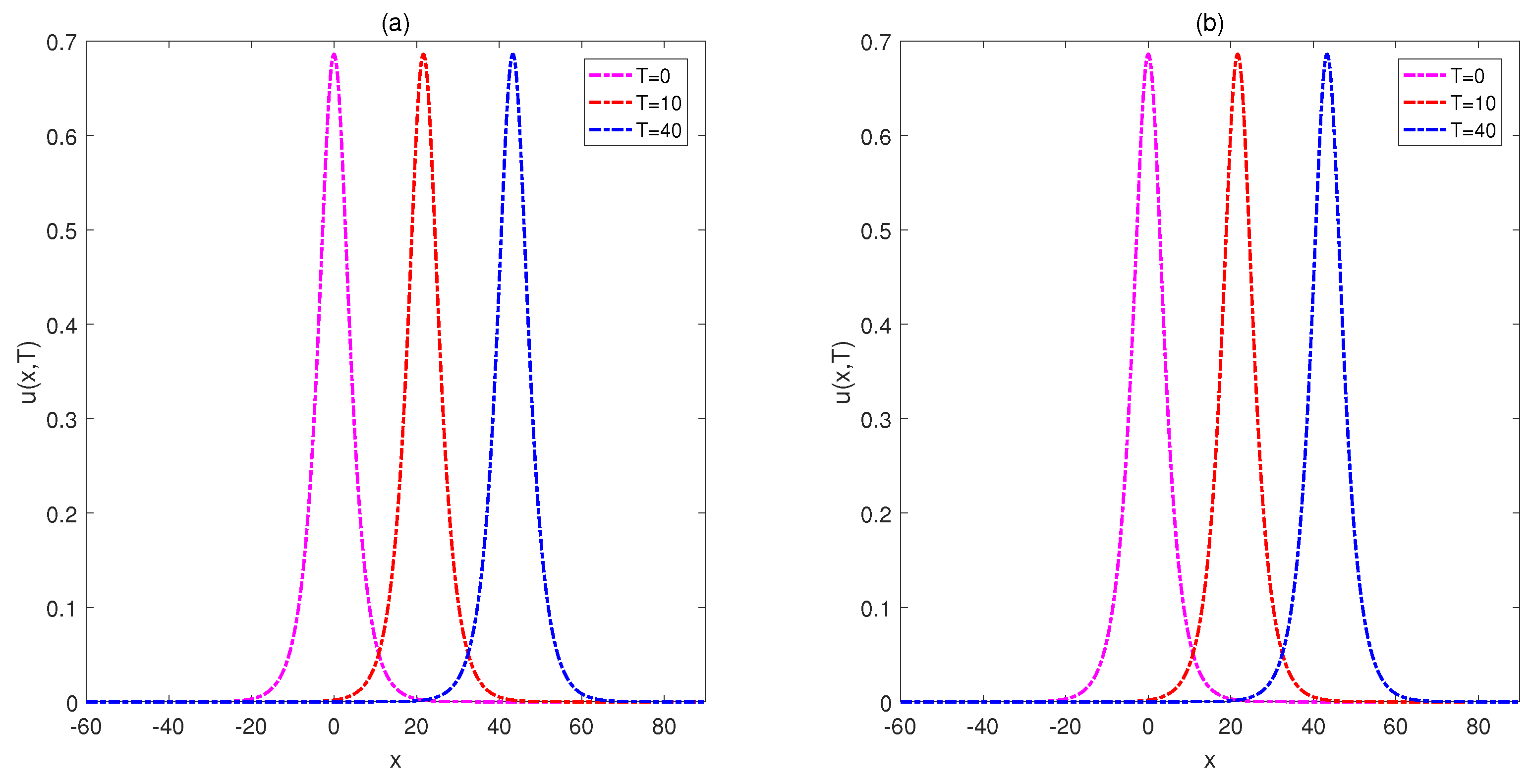
Table 3 reports the $L_{\infty },L_2$ and RMS errors with $\tau =0.01$ and $n_i=489$. Table 4 compares the results with those obtained by the techniques described in [34,41]. It is clear that the results of the new method are considerably more accurate. Table 5 illustrates the conservative law of the discrete energy E. Figure 6 depicts the motion of single solitary wave with $h=\tau =0.125$ (left) and $h=\tau =0.0625$ (right) over the spatial interval $x\in [-60,90]$ at final times $T\in \{0,10,40\}.$ The single solitons move to the right at a constant speed preserving their amplitude and shape. 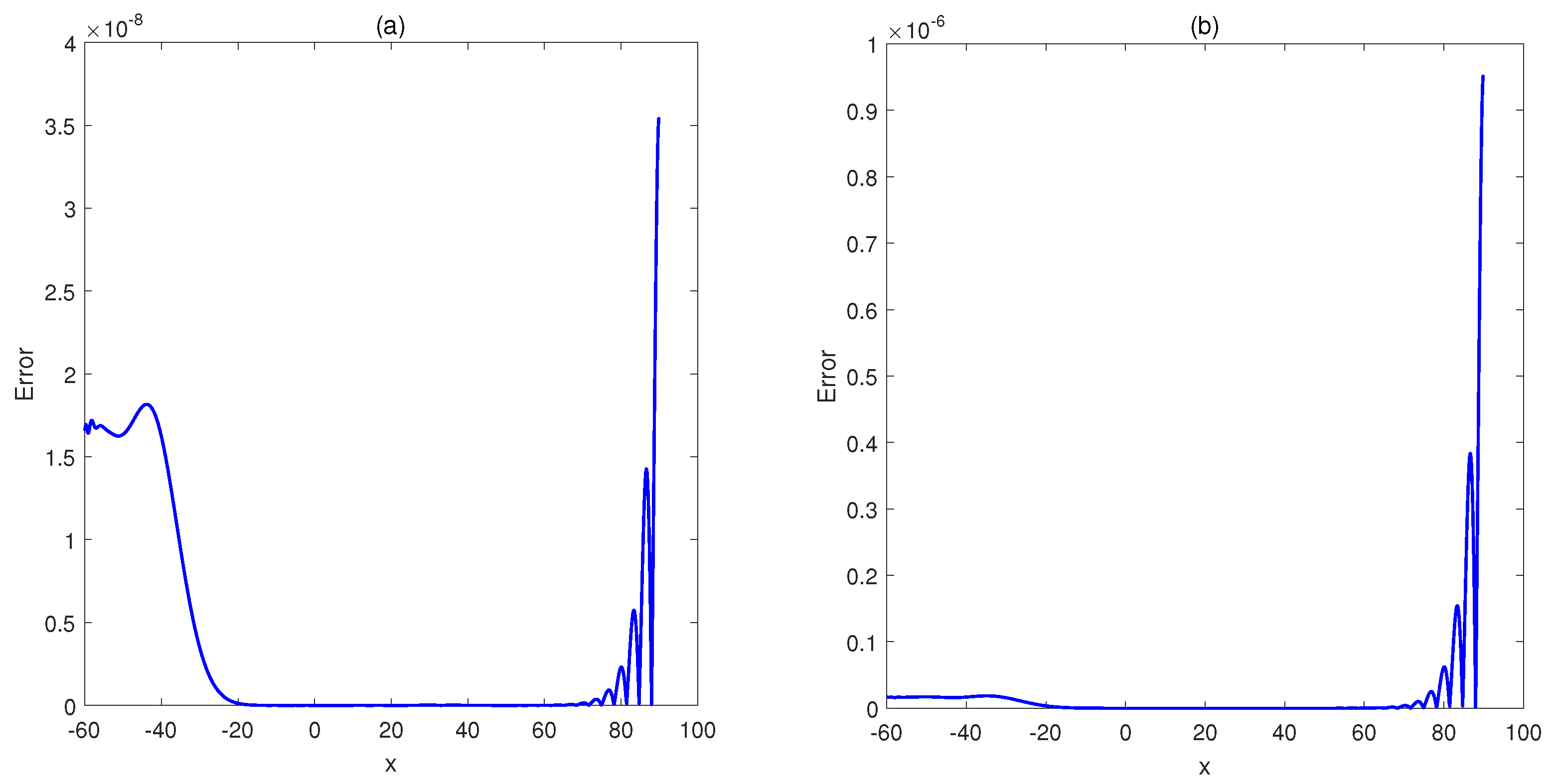Figure 7 represents the absolute error $L_{\infty }$ at final times $T=\{30,40\}$. 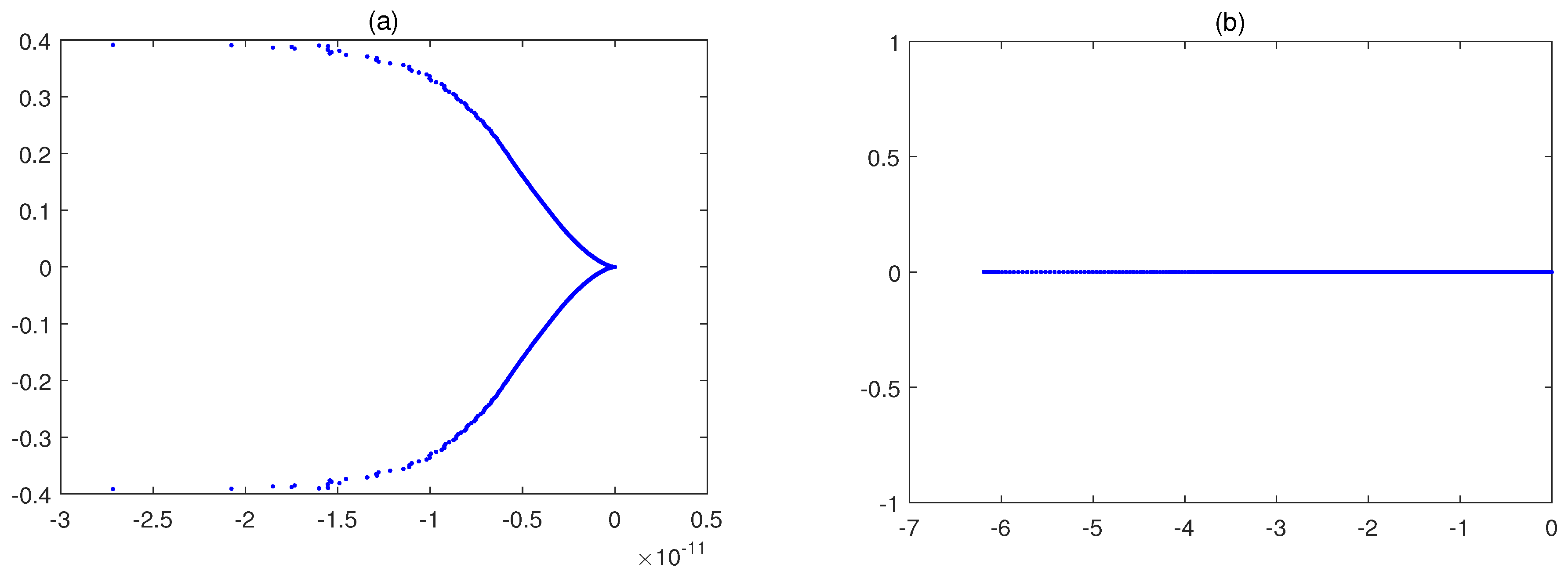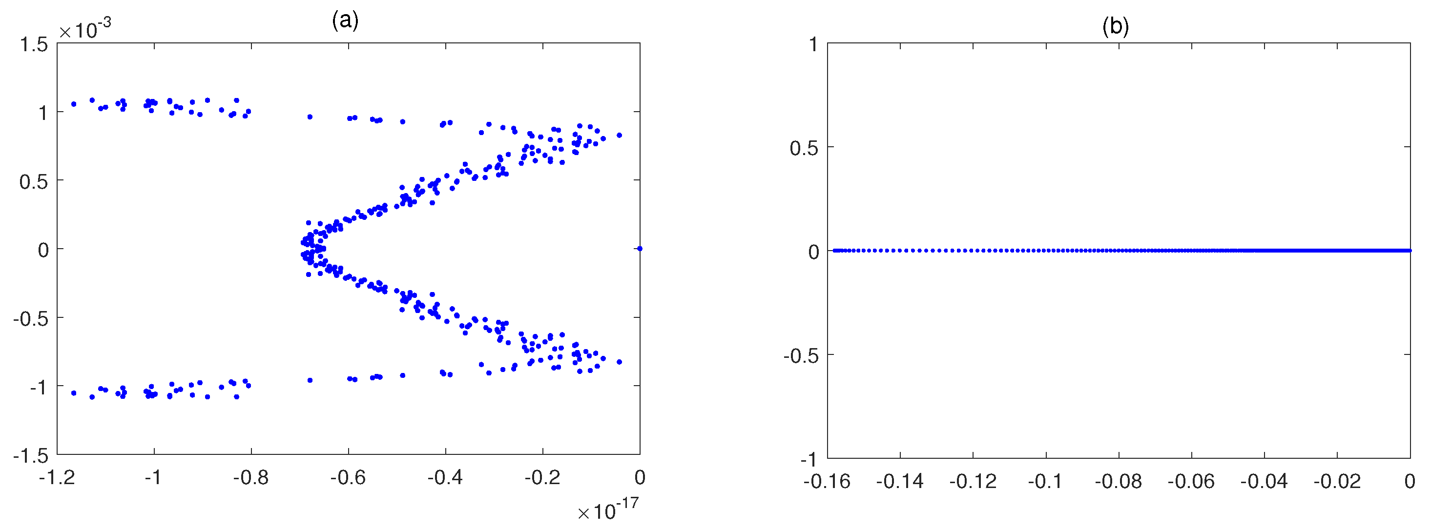Figure 8 plots the eigenvalues of the matrices $\mathbf{A}$ and $\mathbf{B}$ (left and right panels, respectively) with $N=100$. The eigenvalues calculated for $\mathbf{A}$ are negative values. For what concerns $\mathbf{B}$, they are zero or have negative values. Therefore, the stability of the proposed system is confirmed.

Table 3. The $L_{\infty },L_2$ and RMS errors with $\tau =0.01$, $N=900$ and $n_i=489$ for Example 2.

Method	T	c	${\mathit{L}}_{\mathit{\infty }}$	${\mathit{L}}_2$	RMS
RBF-FD	5	1.55	$1.3384\times {10}^{-8}$	$8.7070\times {10}^{-8}$	$1.5499\times {10}^{-9}$
RBF-FD	10	1.55	$1.5966\times {10}^{-8}$	$3.6942\times {10}^{-8}$	$3.0163\times {10}^{-9}$
RBF-FD	15	3.10	$1.7030\times {10}^{-8}$	$5.1031\times {10}^{-8}$	$4.1667\times {10}^{-9}$
RBF-FD	20	2.90	$1.7257\times {10}^{-8}$	$6.3340\times {10}^{-8}$	$5.1717\times {10}^{-9}$
RBF-FD	25	1.80	$1.7608\times {10}^{-8}$	$7.3863\times {10}^{-8}$	$6.0309\times {10}^{-9}$
RBF-FD	30	3.10	$3.5768\times {10}^{-8}$	$9.2721\times {10}^{-8}$	$7.5706\times {10}^{-9}$
RBF-FD	35	3.10	$1.8542\times {10}^{-7}$	$2.3769\times {10}^{-7}$	$1.9407\times {10}^{-8}$
RBF-FD	40	1.55	$9.5039\times {10}^{-7}$	$1.0022\times {10}^{-6}$	$8.1827\times {10}^{-8}$

Table 4. The $L_{\infty }$ and $L_2$ errors under different mesh steps $h=\tau$ at $T=40$ for Example 2.

	Method	c	N	${\mathit{n}}_{\mathit{i}}$	${\mathit{L}}_{\mathit{\infty }}$	${\mathit{L}}_2$
$h=\tau =1/4$
	RBF-FD	2.10	600	569	$1.7483\times {10}^{-8}$	$1.2820\times {10}^{-7}$
	[41]	−	600	−	$1.7999\times {10}^{-2}$	−
	[34]	−	600	−	$9.2311\times {10}^{-3}$	−
$h=\tau =1/8$
	RBF-FD	3.10	1600	869	$1.7234\times {10}^{-8}$	$1.7947\times {10}^{-7}$
	[41]	−	1600	−	$4.5680\times {10}^{-3}$	−
	[34]	−	1600	−	$2.3321\times {10}^{-3}$	−
$h=\tau =1/16$
	RBF-FD	6.80	2400	1541	$1.6718\times {10}^{-8}$	$2.4817\times {10}^{-7}$
	[41]	−	2400	−	$1.1469\times {10}^{-3}$	−
	[34]	−	2400	−	$5.8475\times {10}^{-4}$	−

Table 5. The energy E under different mesh steps $\tau =h$ for Example 2.

	Method	T	c	N	${\mathit{n}}_{\mathit{i}}$	E
$h=\tau =1/4$
	RBF-FD	10	2.6	600	235	6.211055573870
	[41]	10	-	600	-	6.221349804819
	RBF-FD	20	2.6	600	235	6.211055573872
	[41]	20	-	600	-	6.221349804820
	RBF-FD	30	2.6	600	235	6.211055573871
	[41]	30	-	600	-	6.221349804820
	RBF-FD	40	2.6	600	235	6.211055573869
	[41]	40	-	600	-	6.221349804820
$h=\tau =1/8$
	RBF-FD	10	3.1	1200	869	6.216240094383
	[41]	10	-	1200	-	6.221405877565
	RBF-FD	20	3.1	1200	869	6.216240094388
	[41]	20	-	1200	-	6.221405877551
	RBF-FD	30	3.1	1200	869	6.216240094391
	[41]	30	-	1200	-	6.221405877549
	RBF-FD	40	3.1	1200	869	6.216240094396
	[41]	40	-	1200	-	6.216240094397
$h=\tau =0.0625$
	RBF-FD	10	6.8	2400	1541	6.218832354561
	[41]	10	-	2400	-	6.221419928242
	RBF-FD	20	6.8	2400	1541	6.218832354855
	[41]	20	-	2400	-	6.221419928522
	RBF-FD	30	6.8	2400	1541	6.218832354657
	[41]	30	-	2400	-	6.221419928339
	RBF-FD	40	6.8	2400	1541	6.218832354213
	[41]	40	-	2400	-	6.221419928294

Figure 6. Motion of the single solitary wave with $h=\tau =0.125$ (a) and $h=\tau =0.0625$ (b) over the interval $x\in [-60,90]$ at final times $T\in \{0,10,40\}$ for Example 2.

Figure 7. The absolute error $L_{\infty }$ with $\tau =h=0.05,$ at final times $T=30$ (a) and $T=40$ (b) over the interval $x\in [-60,90]$ for Example 2.

Figure 8. The eigenvalues of $\mathbf{A}$ (a) and $\mathbf{B}$ (b) for $N=600$, $n_i=235$ and $c=1.12$ in Example 2.

Example 3.

We consider the general Rosenau-KdV-RLW model (1) corresponding to the case $\alpha =\mu =1$, $\beta =0.5$, $p=2$, $\mu =0.1$ and $\delta =0$ over the spatial interval $x\in [-40,100]$. The exact solution is $u(x,t)=k_{31}{\mathrm{sech}}^4\left[k_{32}(x-k_{33}t)\right]$, where [19]

$$k_{31}=-\frac{5}{456}(25-13\sqrt{457}),k_{32}={\left(\frac{-13+\sqrt{457}}{288}\right)}^{1/2},k_{33}=\frac{241+13\sqrt{457}}{266}·$$

Table 6 compares the results of the proposed method with those resulting from the schemes in [19,41]. The computational efficiency is clearly superior to the performance exhibited by the other schemes. Figure 9 plots the motion of single solitary wave with $h=\tau =0.5,$ (left) $h=\tau =0.25$ (right) over the spatial interval $x\in [-40,100]$ at final times $T\in \{0,30,40\}$. The peak of the solitary waves remains the same during the simulation. Figure 10 shows the eigenvalues of the matrices $\mathbf{A}$ and $\mathbf{B}$ (left and right panel, respectively) with $N=100$. The eigenvalues calculated for $\mathbf{A}$ and $\mathbf{B}$ have zero or negative values. Hence, the stability of the proposed system for this case is confirmed.

Table 6. The $L_{\infty }$ and $L_2$ errors under different mesh steps $h=\tau$ for Example 3.

	Method	T	c	N	${\mathit{n}}_{\mathit{i}}$	${\mathit{L}}_{\mathit{\infty }}$	${\mathit{L}}_2$
$h=\tau =1/2$
	RBF-FD	30	1.71	280	241	$5.3379\times {10}^{-1}$	$2.1555\times {10}^0$
	[19]	30	-	280	-	$9.8675\times {10}^{-1}$	$2.5784\times {10}^0$
$h=\tau =1/4$
	RBF-FD	30	2.90	560	431	$6.5718\times {10}^{-2}$	$3.5432\times {10}^{-1}$
	[41]	30	-	560	-	$6.9960\times {10}^{-1}$	$1.{8662}^0$
	[19]	30	-	560	-	$9.8675\times {10}^{-1}$	$2.9434\times {10}^0$
$h=\tau =1/8$
	RBF-FD	30	5.40	1120	881	$4.2035\times {10}^{-2}$	$1.8697\times {10}^{-2}$
	[41]	30	-	1120	-	$1.9713\times {10}^{-1}$	$5.1866\times {10}^{-1}$
	[19]	30	-	1120	-	$5.1920\times {10}^{-2}$	$8.0563\times {10}^{-1}$

Figure 9. Motion of the single solitary wave with $h=\tau =0.5$ (a) and $h=\tau =0.25$ (b) over the interval $x\in [-40,100]$ at final times $T\in \{0,10,30\}$ (a) and $T\in \{0,20,40\}$ (b) for Example 3.

Figure 10. The eigenvalues of $\mathbf{A}$ (a) and $\mathbf{B}$ (b) for $N=5600$, $n_i=431$ and $c=1.14$ for Example 3.

Example 4.

Let us consider the general Rosenau-KdV-RLW model (1) in the case of $\alpha =\mu =1$, $\beta =1$, $p=2$, $\gamma =0$ and $\delta =1$ over the spatial interval $x\in [-50,150]$ [19,25,33,42]. The exact solution is $u(x,t)=k_{41}{\mathrm{sech}}^4\left[k_{42}(x-k_{43}t)\right]$, where

$$k_{41}=\frac{15}{19},k_{42}=\frac{\sqrt{13}}{26},k_{43}=\frac{169}{133}·$$

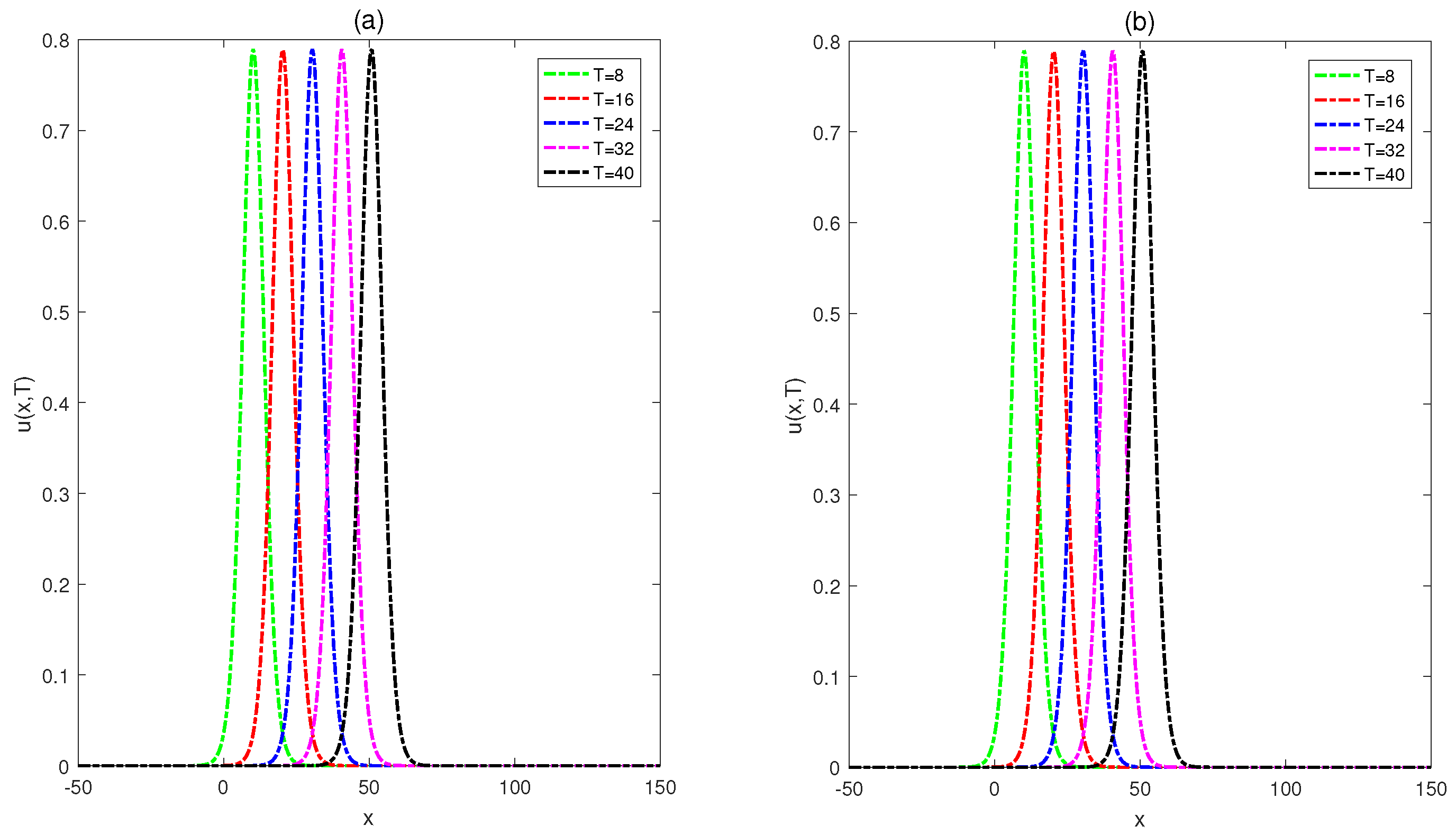
Table 7 compares the results of proposed method with those obtained with other schemes [19,25,33,42]. In this case, the accuracy of the method is slightly better than those achieved with the rest. Figure 11 depicts the motion of the single solitary wave with $h=\tau =0.4$ (left) and $h=\tau =0.2$ (right) over the spatial interval $x\in [-50,150]$ at final times $T\in \{8,16,24,32\}.$ The crest of the soliton clearly remains the same during the simulation. Figure 12 plots the eigenvalues of the matrices $\mathbf{A}$ and $\mathbf{B}$ (left and right panels, respectively) with $N=100$. The eigenvalues calculated for $\mathbf{A}$ are negative values, while for $\mathbf{B}$ they have zero or negative values. Hence, the stability of the proposed system for this case is verified.

Table 7. The $L_{\infty }$ and $L_2$ errors under different mesh steps $h=\tau$ with $N=250$ and $n_i=181$ at $T=24$ for Example 4.

	Method	T	c	N	${\mathit{n}}_{\mathit{i}}$	${\mathit{L}}_{\mathit{\infty }}$	${\mathit{L}}_2$
$h=\tau =0.8$
	RBF-FD	24	0.35	250	181	$1.2281\times {10}^{-11}$	$4.7975\times {10}^{-11}$
	[42]	24	-	250	-	$3.09410\times {10}^{-4}$	$7.78402\times {10}^{-4}$
	[25]	24	-	250	-	$9.06883\times {10}^{-4}$	$2.42851\times {10}^{-1}$
	[33]	24	-	250	-	$1.16717\times {10}^{-1}$	$3.11658\times {10}^{-1}$
	[19]	24	-	250	-	$7.56362\times {10}^{-3}$	$2.03287\times {10}^{-2}$
$h=\tau =0.4$
	RBF-FD	24	0.65	500	381	$1.3151\times {10}^{-11}$	$5.2620\times {10}^{-11}$
	[42]	24	-	500	-	$1.87205\times {10}^{-5}$	$4.73034\times {10}^{-5}$
	[25]	24	-	500	-	$2.48437\times {10}^{-4}$	$6.58790\times {10}^{-2}$
	[33]	24	-	500	-	$3.27045\times {10}^{-2}$	$8.62872\times {10}^{-2}$
	[19]	24	-	500	-	$1.82402\times {10}^{-3}$	$4.88759\times {10}^{-3}$
$h=\tau =0.2$
	RBF-FD	24	1.40	1000	631	$1.3472\times {10}^{-11}$	$5.4481\times {10}^{-11}$
	[42]	24	-	100	-	$1.16521\times {10}^{-6}$	$2.94078\times {10}^{-6}$
	[25]	24	-	1000	-	$6.36404\times {10}^{-3}$	$1.68468\times {10}^{-2}$
	[33]	24	-	1000	-	$8.43616\times {10}^{-3}$	$2.21942\times {10}^{-2}$
	[19]	24	-	1000	-	$4.52324\times {10}^{-4}$	$1.21311\times {10}^{-3}$
$h=\tau =0.1$
	RBF-FD	24	2.60	2000	1831	$1.4086\times {10}^{-11}$	$5.9844\times {10}^{-11}$
	[42]	24	-	2000	-	$7.27778\times {10}^{-8}$	$1.83776\times {10}^{-7}$
	[25]	24	-	2000	-	$1.12985\times {10}^{-4}$	$4.23946\times {10}^{-3}$
	[33]	24	-	2000	-	$3.02978\times {10}^{-4}$	$5.59422\times {10}^{-3}$
	[19]	24	-	2000	-	$2.21651\times {10}^{-3}$	$3.02978\times {10}^{-3}$

Figure 11. Motion of the single solitary wave with $h=\tau =0.4$ (a) and $h=\tau =0.2$ (b) over the interval $x\in [-50,150]$ at final times $T\in \{8,16,24,32\}$ for Example 4.

Figure 12. The eigenvalues of $\mathbf{A}$ (a) and $\mathbf{B}$ (b) for $N=1000$, $n_i=631$, $p=8$ and $c=0.95$ in Example 4.

Example 5.

Consider the general Rosenau-KdV-RLW model (1) with parameters as $\alpha =\beta =\mu =\delta =1$ and $\gamma =0,$ in two spatial intervals, namely $x\in [-60,120]$ and $x\in [-30,120]$. The exact solution is given by

$$u(x,t)=exp\left(k_{51}\right){\mathrm{sech}}^{\frac{4}{p-1}}\left[k_{52}(x-k_{53}t)\right],$$

where

$$\begin{array}{cc}\hfill & k_{51}=(ln\left[(p+3)(3p+1)(p+1)\right]/\left[2(p^2+3)(p^2+4p+7)\right]/(p-1),\hfill \\ \hfill & k_{52}={\displaystyle \frac{p-1}{\sqrt{4p^2+8p+20}}},\hfill \\ \hfill & k_{53}=(p^4+4p^3+14p^2+20p+25)/(p^4+4p^3+10p^2+12p+21).\hfill \end{array}$$

The initial boundary value problem (1)–(3) includes the following conservative quantities:

$$\begin{array}{cc}\hfill & I_1=\frac{1}{2}{\int }_a^{b}u\mathrm{d}x=\frac{h}{2}\sum _{i=1}^N{u}_i,\hfill \\ \hfill & I_2=\frac{1}{2}{\int }_a^b(u^2+u_x^2+u_{xx}^2)\mathrm{d}x=\frac{h}{2}\sum _{i=1}^N\left(u_i+{{\left(u_x\right)}_i}^2+{{\left(u_{xx}\right)}_i}^2\right),\hfill \end{array}$$

related to mass and energy. The quantities $I_1$ and $I_2$ are applied to measure the conservation properties of the present method, calculated by means of the trapezoidal rule for the Rosenau-RLW equation.

Table 8 and Table 9 compare the results of the proposed method with those obtained from the schemes presented in [26,36,37,39]. It can be observed that the computational results are clearly better than the others and that the invariants $I_1$ and $I_2$ remain constant during the simulation. Figure 13 plots the motion of the single solitary wave for various p at $T=\{0,30,60\}$ in the spatial interval $x\in [-60,120]$. The single solitons move to the right at a constant speed and conserve their amplitudes and shapes. Figure 14 shows the eigenvalues of the linearized differentiation operator $\mathbf{A}$ and $\mathbf{B}$ (left and right panels, respectively) with $N=100$. The eigenvalues calculated for $\mathbf{A}$ and $\mathbf{B}$ are zero, or have negative values. Therefore, the stability of the proposed system for this case is confirmed.

Table 8. The $L_{\infty }$, $L_2$ and RMS errors and the invariants $I_1$ and $I_2$ with $N=1500,n_i=1089,c=2.6$ and $\tau =0.01$ in the spatial interval $x\in [-30,120]$ for Example 5.

	Method	T	${\mathit{L}}_{\mathit{\infty }}$	${\mathit{L}}_2$	RMS	${\mathit{I}}_1$	${\mathit{I}}_2$
$p=2$
	RBF-FD	10	$4.2666\times {10}^{-7}$	$1.1117\times {10}^{-6}$	$9.0769\times {10}^{-8}$	$1.89238729$	$0.53169648$
	[37]	10	$7.6292\times {10}^{-6}$	$1.8132\times {10}^{-5}$	−	$1.89765990$	$0.53317753$
	RBF-FD	20	$4.5738\times {10}^{-7}$	$5.3007\times {10}^{-6}$	$1.3686\times {10}^{-7}$	$1.89238729$	$0.53169648$
	[37]	20	$9.0949\times {10}^{-6}$	$2.2513\times {10}^{-5}$	−	$1.89766149$	$0.53317753$
	RBF-FD	30	$4.6844\times {10}^{-7}$	$6.5742\times {10}^{-6}$	$1.6975\times {10}^{-7}$	$1.89238729$	$0.53169648$
	[37]	30	$1.0274\times {10}^{-5}$	$2.5463\times {10}^{-5}$	−	$1.89766306$	$0.53317753$
	RBF-FD	40	$4.7437\times {10}^{-7}$	$7.6096\times {10}^{-6}$	$1.9648\times {10}^{-7}$	$1.89238729$	$0.53169648$
	[37]	40	$1.1378\times {10}^{-5}$	$2.8139\times {10}^{-5}$	−	$1.89766459$	$0.53317753$
	RBF-FD	50	$4.7692\times {10}^{-7}$	$8.4995\times {10}^{-6}$	$2.1946\times {10}^{-7}$	$1.89238729$	$0.53169648$
	[37]	50	$1.2447\times {10}^{-5}$	$3.0753\times {10}^{-5}$	−	$1.89766608$	$0.53317753$
$p=3$
	RBF-FD	10	$3.9146\times {10}^{-6}$	$3.1606\times {10}^{-5}$	$8.1606\times {10}^{-7}$	$2.66518850$	$1.11037761$
	[37]	10	$2.1569\times {10}^{-5}$	$4.9409\times {10}^{-5}$	−	$2.67262472$	$1.11347058$
	RBF-FD	20	$4.2260\times {10}^{-6}$	$4.9004\times {10}^{-5}$	$1.2653\times {10}^{-6}$	$2.66518850$	$1.11037761$
	[37]	20	$2.7517\times {10}^{-5}$	$6.5313\times {10}^{-5}$	−	$2.67264006$	$1.11347058$
	RBF-FD	30	$4.3421\times {10}^{-6}$	$6.1274\times {10}^{-5}$	$1.5821\times {10}^{-6}$	$2.66518850$	$1.11037761$
	[37]	30	$3.3326\times {10}^{-5}$	$7.9999\times {10}^{-5}$	−	$2.67265504$	$1.11347058$
	RBF-FD	40	$4.4063\times {10}^{-6}$	$7.1244\times {10}^{-5}$	$1.8395\times {10}^{-6}$	$2.66518850$	$1.11037761$
	[37]	40	$3.9091\times {10}^{-5}$	$9.4787\times {10}^{-5}$	−	$2.67266966$	$1.11347058$
	RBF-FD	50	$4.4481\times {10}^{-6}$	$7.6096\times {10}^{-6}$	$2.0648\times {10}^{-6}$	$2.66518850$	$1.11037761$
	[37]	50	$4.4846\times {10}^{-5}$	$1.0984\times {10}^{-4}$	−	$2.67268415$	$1.11347058$
$p=6$
	RBF-FD	10	$3.3603\times {10}^{-4}$	$8.0524\times {10}^{-4}$	$6.5626\times {10}^{-5}$	$3.97819339$	$1.91229616$
	[37]	10	$3.1032\times {10}^{-4}$	$6.5998\times {10}^{-4}$	−	$3.99024365$	$1.91764461$
	RBF-FD	20	$3.6994\times {10}^{-4}$	$1.3622\times {10}^{-3}$	$1.1107\times {10}^{-4}$	$3.97819339$	$1.91229616$
	[37]	20	$3.1897\times {10}^{-4}$	$1.1382\times {10}^{-3}$	−	$3.99024365$	$1.91764461$
	RBF-FD	30	$3.8386\times {10}^{-4}$	$1.7513\times {10}^{-3}$	$1.4281\times {10}^{-4}$	$3.97819339$	$1.91229616$
	[37]	30	$3.2836\times {10}^{-4}$	$1.4631\times {10}^{-3}$	−	$3.99172706$	$1.91764489$
	RBF-FD	40	$3.9219\times {10}^{-4}$	$2.0639\times {10}^{-3}$	$1.6841\times {10}^{-4}$	$3.97819339$	$1.91229616$
	[37]	40	$3.4181\times {10}^{-4}$	$1.7187\times {10}^{-3}$	−	$3.99458409$	$1.91764541$
	RBF-FD	50	$3.9792\times {10}^{-4}$	$2.3398\times {10}^{-3}$	$1.9060\times {10}^{-4}$	$3.99484237$	$1.91634750$
	[37]	50	$3.4127\times {10}^{-4}$	$1.9368\times {10}^{-3}$	−	$3.99597486$	$1.91764566$

Table 9. The $L_{\infty }$ and $L_2$ errors and the quantities Q and E with $N=360,n_i=295,c=0.55$ and $\tau =0.1$ in the spatial interval $x\in [-60,120]$ for Example 5.

	Method	${\mathit{L}}_{\mathit{\infty }}$	${\mathit{L}}_2$	Q	E
$p=4$
	RBF-FD	$4.1402\times {10}^{-10}$	$2.1363\times {10}^{-9}$	6.248401	2.859729
	[39]	$1.3784\times {10}^{-4}$	$9.3510\times {10}^{-4}$	6.266377	2.868226
	[39]	$1.0310\times {10}^{-5}$	$2.3550\times {10}^{-5}$	6.265844	2.867735
	[39]	$2.9706\times {10}^{-4}$	$6.6954\times {10}^{-4}$	6.265806	2.867684
	[39]	$4.2250\times {10}^{-4}$	$1.1045\times {10}^{-3}$	6.265992	2.867617
	[26]	$1.7112\times {10}^{-3}$	$4.4788\times {10}^{-3}$
	[36]	$2.7871\times {10}^{-2}$	$7.4517\times {10}^{-2}$
$p=8$
	RBF-FD	$2.7865\times {10}^{-6}$	$1.4924\times {10}^{-5}$	9.745127	4.722011
	[39]	$1.3784\times {10}^{-4}$	$3.8078\times {10}^{-4}$	9.742126	4.735346
	[39]	$2.9490\times {10}^{-5}$	$7.5220\times {10}^{-5}$	9.742181	4.735225
	[39]	$6.2856\times {10}^{-4}$	$1.7039\times {10}^{-3}$	9.742146	4.735302
	[39]	$4.7892\times {10}^{-4}$	$1.2762\times {10}^{-3}$	9.742227	4.735082
	[26]	$1.6189\times {10}^{-3}$	$4.3184\times {10}^{-3}$
	[36]	$2.9534\times {10}^{-2}$	$8.0373\times {10}^{-2}$
$p=16$
	RBF-FD	$9.1964\times {10}^{-4}$	$4.8646\times {10}^{-3}$	17.167390	8.372094
	[39]	$4.4109\times {10}^{-4}$	$2.3334\times {10}^{-3}$	17.168699	8.375376
	[39]	$4.4493\times {10}^{-4}$	$2.3199\times {10}^{-3}$	17.169258	8.375400
	[39]	$5.3860\times {10}^{-4}$	$3.0231\times {10}^{-3}$	17.172776	8.375393
	[39]	$2.2709\times {10}^{-3}$	$7.6218\times {10}^{-3}$	17.116828	8.375272
	[26]	$1.1875\times {10}^{-3}$	$3.5725\times {10}^{-3}$
	[36]	$2.2547\times {10}^{-2}$	$6.1304\times {10}^{-2}$

Figure 13. Motion of the single solitary wave for $p=3$ (a), $p=6$ (b), $p=4$ (c), and $p=8$ (d) at final times $T\in \{0,30,60\}$ (a,b) and $T\in \{0,20,40\}$ (c,d) in the spatial interval $x\in [-60,120]$ for Example 5.

Figure 14. The eigenvalues of $\mathbf{A}$ (a) and $\mathbf{B}$ (b) for $N=500$, $n_i=111$ and $c=1.26$ in Example 5.

4. Conclusions

We adopted the local meshless RBF-FD to calculate the approximate numerical solutions of the general nonlinear Rosenau-RLW equation without performing any linearization or transformation of the equation. In order to demonstrate the accuracy of the proposed numerical technique, the error invariants and error norms were computed, and the results were compared with others available in the literature. The local RBF-FD technique was verified to be remarkably accurate. In conclusion, the method is sufficiently accurate and fast due to its limited computational load.