Approximations in Performance Analysis of a Controllable Queueing System with Heterogeneous Servers

Abstract

The paper studies a controllable multi-server heterogeneous queueing system where servers operate at different service rates without preemption, i.e., the service times are uninterrupted. The optimal control policy allocates the customers between the servers in such a way that the mean number of customers in the system reaches its minimal value. The Markov decision model and the policy-iteration algorithm are used to calculate the optimal allocation policy and corresponding mean performance characteristics. The optimal policy, when neglecting the weak influence of slow servers, is of threshold type defined as a sequence of threshold levels which specifies the queue lengths for the usage of any slower server. To avoid time-consuming calculations for systems with a large number of servers, we focus here on a heuristic evaluation of the optimal thresholds and compare this solution with the real values. We develop also the simple lower and upper bound methods based on approximation by an equivalent heterogeneous queueing system with a preemption to measure the mean number of customers in the system operating under the optimal policy. Finally, the simulation technique is used to provide sensitivity analysis of the heuristic solution to changes in the form of inter-arrival and service time distributions.

1. Introduction

The study of multi-server queueing systems in most cases assumes the servers to be homogeneous when the individual service rates are the same for all the servers in the system. However, in many real applications, the assumption of the homogeneity cannot be valid, e.g., a group of servers with different types of processors as a consequence of irregular system updates, nodes in telecommunication networks with links of different unequal capacities and availability, nodes in wireless systems serving different mobile users, peer-to-peer services for data streaming, file sharing and storage, where heterogeneous servers arrive and depart randomly, multi-processor systems with heterogeneous processor’s attributes like a throughput and an electric energy consumption, etc. Moreover, in many cases the heterogeneous server system outperforms its homogeneous server counterpart. This reality leads to necessity to analyse multi-server queueing systems with heterogeneous servers. The assumption of the heterogeneity of servers does not automatically mean that the stochastic modelling of such a queueing system becomes more complex. If the customers can change the server to a faster one during a service, in other words, the service is with a preemption, this is a classic one-dimensional birth-and-death process, that can be analysed in a standard way. The task of analysing a heterogeneous system becomes much more complex with the assumption that the customer cannot change the server during a service time, i.e., service without any preemption. In this case, on the one hand, the dimension of the corresponding random process increases and on the other hand, a mechanism for allocation of customers between the servers must be introduced.

The systems with heterogeneous servers are mostly investigated with respect to heuristic allocation policies, e.g., allocation according to the fastest server first (FSF) policy or the randomly chosen server (RCS). The results dedicated to the heterogeneous systems operating under these policies and some approximations of such models can be found in papers of Alves et al. [1], Bilgen and Altintas [2], Melikov et al. [3], The question of how to allocate the customers between the heterogeneous servers in order to minimize the mean number of customers in the system was studied for the queueing system with two servers in terms of a Markov decision process (MDP), e.g., by Larsen [4], Larsen and Agrawala [5], who conjectured the optimality of threshold policy that functions as follows: the fastest server must be used whenever it is idle and the slower one must be used only if the number of customers in the queue exceeds some prespecified threshold level $q\ge 1$. Based on the MDP model, Lin and Kumar in [6] considered a similar problem and proved the optimality of a threshold policy. Simple proofs of corresponding results have later been given by Koole [7], Luh and Viniotis [8], Walrand [9] and Weber [10]. The problem of an optimal control of a two-server queueing system with failures was studied by Özkan and Kharoufeh [11]. The problem of the optimal control allocation in the systems with more than two servers were investigated by Armony and Ward [12], Efrosinin [13], Rosberg and Makowski [14], Viniotis and Ephremides [15]. Rykov in [16] gave evidence for certain monotonicity properties of an optimal policy in case of the mean number of customers minimization. The techniques to prove such results are based on monotonicity properties of the dynamic programming relative value function. The case of infinitely many servers was proposed by Shenker and Weinrib [17], where an asymptotic analysis of large heterogeneous queueing systems is performed.

As it was shown in [18,19], also taking into account the incompleteness of the theoretical proof noticed by Vericourt and Zhou in [20], the optimal allocation policy, which minimizes the mean number of customers in heterogeneous queueing system without preemption, belongs to a set of structural policies. According to this policy for the servers’ enumeration (1) the first server is used whenever it is free and there is a waiting customer in the queue, while the empty server with a number $k+1$ must be occupied only if the first k faster servers are busy and the number of customers in the queue reaches some threshold level $q_{k+1}\ge 1$. Numerical analysis shows that the threshold level $q_k$ in general case can have a very weak dependence of slower servers’ states. Due to our observations, the optimal threshold may vary by at most 1 when the state of a slower server changes. Moreover, since this deviation has no influence on the mean number of customers in the system, it can be neglected. Hence the optimal allocation policy can be defined as a classic threshold one through a sequence of threshold levels $1=q_1\le q_2\le \dots \le q_K<\infty$, that is the first k servers must be occupied whenever there are q customers in the queue and $q_k\le q\le q_{k+1}-1$.

While there is a certain amount of work being done on heterogeneous systems, there are still many open questions related to the accurate and quick calculation of the optimal control policy and the resulting performance characteristics. Searching for optimal values $q_2,\dots ,q_K$ by a direct minimizing the mean number of customers in the system can be performed only for small K by solving the system of difference equations for the steady-state probabilities or by means of a matrix geometric approach introduced by Neuts [21]. However, when K is large, these methods become too complicated. For example, the involved in computation matrix sizes become infeasible large even for the moderate numbers of servers like $K\ge 4$, see e.g., [22]. To calculate the optimal threshold levels the MDP model and a policy iteration algorithm [23,24,25], which constructs a sequence of improved policies that converges to optimal one, can also be used. While this approach is a powerful tool for solving many optimization tasks, it has significant limitations on dimension of the model, number of states, convergence in a heavy traffic case due to processing time and memory requirements. The contribution of the paper is three-fold. First, we provide a simple heuristic solution (HS) for a sub-optimal policy in order to avoid the time-consuming search for the optimal one in case of an arbitrary number of servers. Second, we investigate the possibility to use the equivalent queueing system with a preemption and a threshold-based policy to evaluate the lower and upper boundaries for the optimal mean number of customers in the system without preemption. Third, we check by means of a simulation, whether the proposed heuristic solution for the optimal thresholds is insensitive to changes in the form of inter-arrival and service time distributions.

This paper is organized as follows. In Section 2 we discuss a queueing model, formulate the corresponding MDP and specify a policy-iteration algorithm used for evaluation the optimal threshold policy. Section 3 introduces a heuristic solution for the optimal threshold levels based on a simple discrete fluid approximation, that turn out to be nearly optimal. In Section 4 we propose approximations to calculate the lower and upper bounds for the mean number of customers in the system under the optimal allocation policy. In Section 5 the simulation is used to provide sensitivity analysis of the heuristic solution to changes in inter-arrival and service time distributions. Finally, we make some conclusions and remarks.

2. Mathematical Model and MDP Formulation

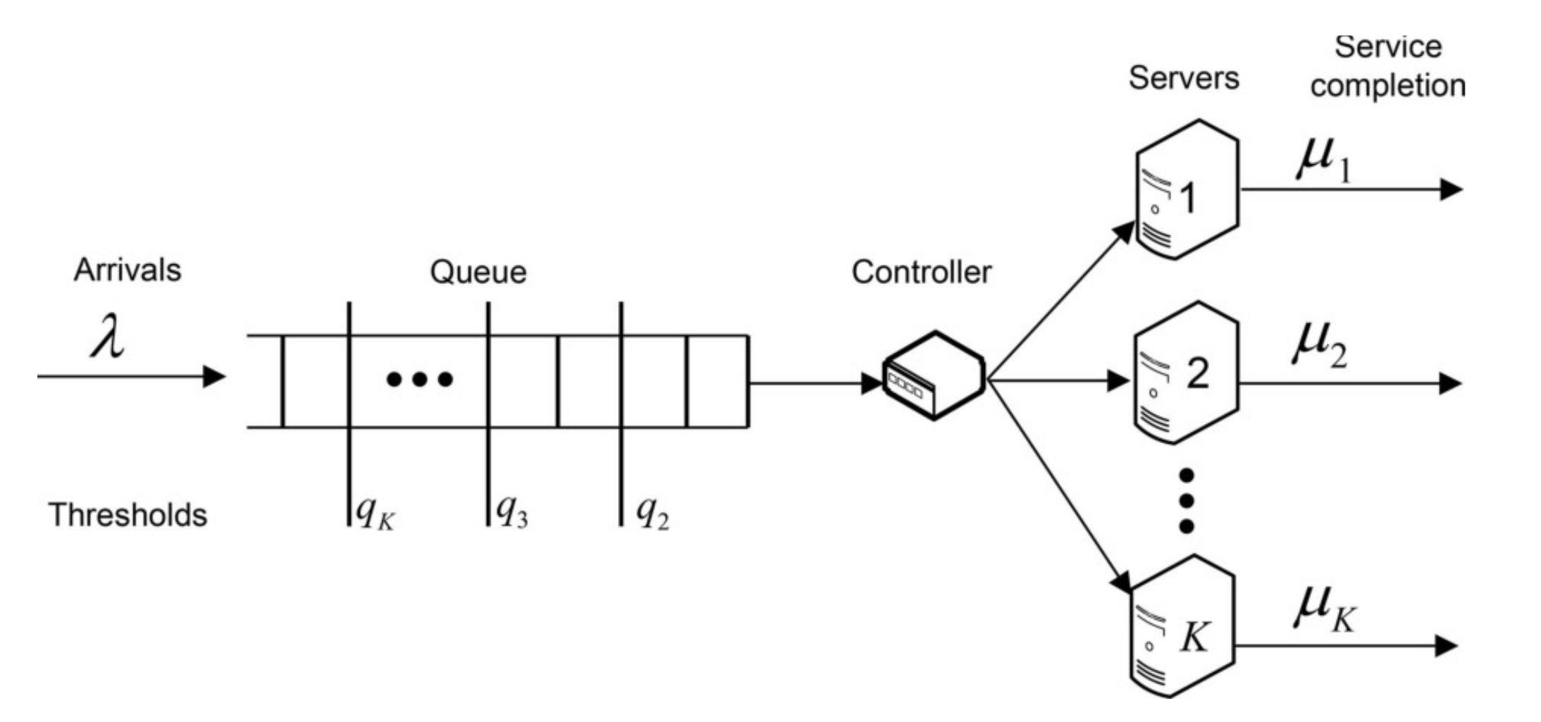
Consider an infinite-capacity $M/M/K$ queueing system with K heterogeneous servers and one common queue, see Figure 1. The customers arrive to the system according to a homogeneous Poisson process with a rate $\lambda$. The jth server has an exponentially distributed service time with a rate ${\mu }_j$. The server j is called an available server if it is idle. The service of customers is has no preemption, i.e., a customer being served on a server cannot change it. In this case a threshold-based policy defined below which is used for the customer allocation has sense. The inter-arrival and service times are assumed to be mutually independent. Assume that the servers are enumerated in a way

$$\begin{array}{c}\hfill {\mu }_1\ge \dots \ge {\mu }_K.\end{array}$$

(1)

The stability condition is obviously defined through the inequality

$$\begin{array}{c}\hfill \lambda <\sum _{j=1}^K{\mu }_j.\end{array}$$

(2)

The controller or decision maker has a full information about system states. It allocates customers between servers according to a control policy f either to one of available servers or to queue at a new arrival and service completion epoch if it occurs with a nonempty queue. The system dynamics is common for the systems with one common queue and heterogeneous servers. At each arrival epoch the customer joins the queue and the controller can allocate the customer staying at the head of the queue to an available server j. At service completion epochs the controller may decide to allocate the customer from the head of nonempty queue to an available server or leave the customer in the queue. As it was mentioned above, the optimal control policy f, which minimizes the mean number of customers in the system with servers ordered according to (1), belongs to a set of threshold policies defined as a sequence of threshold levels

$$\begin{array}{c}\hfill 1=q_1\le q_2\le \dots \le q_K<\infty .\end{array}$$

(3)

According to this policy the first k servers must be occupied whenever there are q customers in the queue and $q_k\le q\le q_{k+1}-1$ for $k=1,\dots ,K-1$, and $q_k\le q<\infty$ for $k=K$. For example, the policy f for the system $M/M/5$ with $K=5$ servers and thresholds $(q_1,q_2,\dots ,q_5)=(1,3,4,5,12)$ means that the fastest server is used whenever upon arrival of a customer it is free and there are q customers in the queue with $1\le q\le 2$. The first two servers are used when $q=3$. The first three servers must be occupied whenever there are $q=4$ customers in the queue, the first four customers are used when $5\le q\le 11$. All servers must be used when the queue length exceeds the level $q\ge 12$. When the queue length drops below a specific threshold level, then the corresponding busy server remains idle after a service completion. As thresholds can take on different values, there are a huge number of admissible threshold policies. Hence the main goal is to calculate the optimal values for threshold levels $q_k$ and the minimized mean number of customers in the system.

We formulate the above optimization problem as a Markov decision process associated with a multi-dimensional continuous-time Markov chain

$$\begin{array}{c}\hfill {\left\{X\left(t\right)\right\}}_{t\ge 0}={\{Q\left(t\right),D_1\left(t\right),\dots ,D_K\left(t\right)\}}_{t\ge 0}\end{array}$$

(4)

with a set of admissible actions $A=\{0,1,\dots ,K\}$ with elements a, where $a=0$ means the allocation of the customer to the queue and $a=j\ne 0$–to the jth server. The term $Q\left(t\right)\in {\mathbb{N}}_0$ in (4) denotes the number of customers in the queue at time t, $D_j\left(t\right)\in \{0,1\}$–the state of server j at time t, where

$$D_j\left(t\right)=\left\{\begin{array}{cc}0\hfill & \mathrm{if}\mathrm{server}j\mathrm{is}\mathrm{idle}\hfill \\ 1\hfill & \mathrm{if}\mathrm{server}j\mathrm{is}\mathrm{busy}.\hfill \end{array}\right.$$

For any fixed allocation policy f we wish to guarantee that the process ${\left\{X\left(t\right)\right\}}_{t\ge 0}$ is an irreducible, positive recurrent Markov chain with a state space $E=\{x=(q\left(x\right),d_1\left(x\right),\dots ,d_K\left(x\right))\}\equiv {\mathbb{N}}_0\times {\{0,1\}}^K$ and infinitesimal generator ${\mathsf{\Lambda }}^f$ which depend on the policy f. The notations $q\left(x\right)$ and $d_j\left(x\right)$ will be used further in the paper to specify the components of the vector state $x\in E$, where $q\left(x\right)$ denotes the queue length in state x and $d_j\left(x\right)$–the state of the jth server in state x. We use next the notations

$$J_0\left(x\right)=\{j:d_j\left(x\right)=0\},J_1\left(x\right)=\{j:d_j\left(x\right)=1\}$$

to specify respectively a set of idle and busy servers in state x, $A\left(x\right)=J_0\left(x\right)\cup \left\{0\right\}\subseteq A$ the subset of admissible actions in state x and ${\mathbf{e}}_j$ stands for a vector of dimension $K+1$ with 1 in the jth position ($j=0,1,\dots ,K$) and 0 elsewhere.

For the ergodic Markov decision process a long-run average cost in the system per unit of time for the policy f coincides with the corresponding assemble average, i.e.,

$$\begin{array}{c}\hfill g^f=\underset{t\to \infty }{lim\; sup}\frac{1}{t}{V}^f(x,t)=\sum _{y\in E^f}l\left(y\right){\pi }_y^f<\infty ,\end{array}$$

(5)

where $l\left(y\right)=q\left(y\right)+{\sum }_{j=1}^K{d}_j\left(y\right)$ in our model is a number of customers in state $y\in E$,

$$\begin{array}{c}\hfill V^f(x,t)={\mathbb{E}}^f\left[{\int }_0^t\left(Q\left(t\right)+\sum _{j=1}^K{D}_j\left(t\right)\right)dt|X\left(0\right)=x\right]\end{array}$$

denotes the total average number of customers up to time t given initial state is x and ${\pi }_y^f={\mathbb{P}}^f[X\left(t\right)=y]$ is a stationary state probability of the process under given policy f. The policy $f^{*}$ is said to be optimal when for $g^f$ defined in (5) we evaluate

$$\begin{array}{c}\hfill g^{*}=\underset{f}{inf}{g}^f=\underset{q_2,\dots ,q_K}{min}g(q_2,\dots ,q_K).\end{array}$$

(6)

One fruitful approach to finding optimal policy $f^{*}$ is through solving the Bellman’s optimality equation, which in our case is of the form

$$\begin{array}{c}\hfill Bv\left(x\right)=(\lambda +\sum _{j\in J_1\left(x\right)}{\mu }_j)v\left(x\right)+g,\end{array}$$

(7)

where B is a dynamic programming operator acting on a relative value function $v:E\to \mathbb{R}$ which indicates a transient effect of an initial state x to the total average cost, and, according to Howard [23], the following asymptotic relation for the function $V^f(x,t)$ in case of a Markov-chain with one ergodic class holds,

$$\begin{array}{c}\hfill V^f(x,t)=g^{f}t+v^f\left(x\right)+o\left(1\right),x\in E,t\to \infty .\end{array}$$

(8)

The functions $v^f$ and $g^f$ further in the paper will be denoted by v and g without upper index f.

Proposition 1. 

The Bellman’s optimality Equation (7) is defined as follows

$$\begin{array}{cc}\hfill Bv\left(x\right)& =l\left(x\right)+\lambda \underset{a\in A\left(x\right)}{min}v(x+{\mathbf{e}}_a)+\sum _{j\in J_1\left(x\right)}{\mu }_{j}v(x-{\mathbf{e}}_j)1_{\left\{q\right(x)=0\}}+\hfill \\ \hfill & +\sum _{j\in J_1\left(x\right)}{\mu }_j\underset{a\in A(x-{\mathbf{e}}_j-{\mathbf{e}}_0)}{min}v(x-{\mathbf{e}}_j-{\mathbf{e}}_0+{\mathbf{e}}_a)1_{\left\{q\right(x)>0\}},\hfill \end{array}$$

(9)

where the notation $1_{\left\{A\right\}}$ specifies the indicator function, which takes the value 1 if the event A holds, and 0 otherwise.

Proof. 

According to [26], the behaviour of the function $V(x,t)$ in the interval $[t,t+dt)$ by letting $t\to \infty$ and taking into account the asymptotic relation (8) can be represented as a system of linear equations, which in general case is of the form

$$v\left(x\right)=\underset{a}{min}\left\{\frac{1}{{\lambda }_x\left(a\right)}\left[c\left(x\right)+\sum _{y\ne x}{\lambda }_{xy}\left(a\right)v\left(y\right)-g\right]\right\}.$$

Evaluating these equations for analyzed queueing system and taking into account the transition rates of the specified Markov decision model we get

$$v\left(x\right)=\frac{1}{\lambda +{\sum }_{j\in J_1\left(x\right)}{\mu }_j}[Bv\left(x\right)-g].$$

The relation for $Bv\left(x\right)$ contains the term $l\left(x\right)$ specifying a number of customers in state $x\in E_X$, the second term represents the changing of the state accompanying with a new arrival which occurs with a rate $\lambda$. The third and the fourth terms represent transitions due to service completions at server j with a rate ${\mu }_j$ by en empty and non-empty queue respectively. □

To generate a data-set for the queueing system under study which includes optimal threshold levels and corresponding values of the system parameters the policy-iteration Algorithm 1 is used. For numerical results the truncated equivalent system with a buffer size W is considered. The algorithm consists of two main steps: policy evaluation and policy improvement. In the first step, for a given control policy f the system of linear equations for the relative value function $v\left(x\right)$, $x\in E\setminus \left\{\right(0,0,\dots ,0\left)\right\}$ must be solved together with an equation $g=\lambda v\left({\mathbf{e}}_1\right)$. In the second step, the obtained in the first step relative function is used to improve the current policy. The algorithm stops when a new policy coincides with a previous one. As an initial policy the FSF allocation policy is used.

Algorithm 1 Policy-iteration algorithm

1: procedure PIA($K,W,\lambda ,{\mu }_j,j=1,2,\dots ,K$) 2:   $f^{\left(0\right)}\left(x\right)={argmax}_{j\in J_0\left(x\right)}\left\{{\mu }_j\right\}$                           ▹ Initial policy 3:   $n\leftarrow 0$ 4:   $g^{\left(n\right)}\leftarrow \lambda v^{\left(n\right)}\left({\mathbf{e}}_1\right)$                           ▹ Policy evaluation 5:   for $x=(0,1,0,\dots ,0) \mathbf{to} (N,1,1,\dots ,1)$ do 6:      $$\begin{array}{cc}\hfill v^{\left(n\right)}\left(x\right)& \leftarrow \frac{1}{\lambda +{\sum }_{j\in J_1\left(x\right)}{\mu }_j}[l\left(x\right)-g^{\left(n\right)}+\lambda v^{\left(n\right)}(x+{\mathbf{e}}_{f^{\left(n\right)}\left(x\right)})\hfill \\ & +\sum _{j\in J_1\left(x\right)}{\mu }_j{v}^{\left(n\right)}(x-{\mathbf{e}}_j)1_{\left\{q\right(x)=0\}}\hfill \\ & +\sum _{j\in J_1\left(x\right)}{\mu }_j{v}^{\left(n\right)}(x-{\mathbf{e}}_j-{\mathbf{e}}_0+{\mathbf{e}}_{f^{\left(n\right)}(x-{\mathbf{e}}_j-{\mathbf{e}}_0)})1_{\left\{q\right(x)>0\}}]\hfill \end{array}$$ 7:   end for 8:                                    ▹ Policy improvement           $$f^{(n+1)}\left(x\right)\leftarrow {argmin}_{a\in A\left(x\right)}{v}^{\left(n\right)}(x+{\mathbf{e}}_a)$$ 9:   if $f^{(n+1)}\left(x\right)\leftarrow f^{\left(n\right)}\left(x\right),x\in E$ then return $f^{(n+1)}\left(x\right),v^{\left(n\right)}\left(x\right),g^{\left(n\right)}$ 10:   else  $n\leftarrow n+1$, go to step 4 11:   end if 12: end procedure

We convert by implementing the Algorithm 1 the $K+1$-dimensional state space E of the Markov decision process ordered in a certain way to a one-dimensional equivalent state space ${\mathbb{N}}_0$, $\Delta :E\to {\mathbb{N}}_0$, for state $x=(q\left(x\right),d_1\left(x\right),\dots ,d_K\left(x\right))\in E$,

$$\begin{array}{c}\hfill \Delta \left(x\right)=q\left(x\right)2^K+\sum _{i=1}^K{d}_i\left(x\right)2^{i-1}.\end{array}$$

(10)

Therefore, in one-dimensional case the changing of the state x due to adding or removing a customer from the queue and due to occupation or departure of a customer from the jth server can be respectively represented in the form,

$$\begin{array}{cc}\hfill & \Delta (x\pm {\mathbf{e}}_0)=(q\left(x\right)\pm 1)2^K+\sum _{i=1}^K{d}_i\left(x\right)2^{i-1}=\Delta \left(x\right)\pm 2^K,\hfill \\ \hfill & \Delta (x\pm {\mathbf{e}}_j)=q\left(x\right)2^K+\sum _{i=1}^K{d}_i\left(x\right)2^{i-1}\pm 2^{j-1}=\Delta \left(x\right)\pm 2^{j-1},j=1,2,\dots ,K.\hfill \end{array}$$

For further details about derivation of the dynamic programming equation needed to evaluate the optimal policy the interested readers are referred to [13]. The infinite buffer queueing system is approximated by a finite buffer equivalent system in such a way that the loss probability does not exceed some specified small number $\epsilon >0$.

Remark 1. 

For the bounded buffer size W the number of states is

$$\left|E\right|=2^K(W+1).$$

If the queue length $q\ge q_K$, all servers must be busy and the system behaves like a $M/M/1$ queueing system with a service rate ${\sum }_{j=1}^K{\mu }_j$. The stationary state probabilities ${\pi }_{(q,1,\dots ,1)}$, $q\ge q_K$, satisfy the difference equation

$$\lambda {\pi }_{(q-1,1,\dots ,1)}-\left(\lambda +\sum _{j=1}^K{\mu }_j\right){\pi }_{(q,1,\dots ,1)}+\sum _{j=1}^K{\mu }_j{\pi }_{(q+1,1,\dots ,1)}=0,$$

which has a solution in a geometric form, ${\pi }_{(q,1,\dots ,1)}={\pi }_{(q_K,1,\dots ,1)}{\rho }^{q-q_K}$, $q\ge q_K$. For details and theoretical substantiation see e.g., [27]. The threshold level $q_K$ can be estimated using HS (11). The buffer size W is chosen in such a way that it satisfies the condition for the loss probability

$$\sum _{q=W}^{\infty }{\pi }_{(q,1,\dots ,1)}={\pi }_{q_K}\sum _{q=W}^{\infty }{\rho }^{q-q_K}\le \sum _{q=W}^{\infty }{\rho }^{q-q_K}=\frac{{\rho }^{W-q_K}}{1-\rho }<\epsilon ,$$

where $\rho =\frac{\lambda }{{\sum }_{j=1}^K{\mu }_j}$. After simple algebra it implies

$$W>\frac{log\epsilon (1-\rho )}{log\left(\rho \right)}+q_K.$$

The algorithm was implemented in C++ and tested for model problems up to 10 servers and a queue of size $W=100$. It shows matching results to the proposed heuristic solution but is only viable for relative small number of servers. For system with 100 servers the maximum number of states would be in the order of $2^{100}$ which makes a reasonable usage of the policy-iteration algorithm impossible.

Example 1. 

Consider the system $M/M/5$ with $K=5$ and $\lambda =15$. The service rates take the following values: $({\mu }_1,{\mu }_2,{\mu }_3,{\mu }_4,{\mu }_5)=$$(20,8,4,2,1)$. The buffer size is $W=80$ which for $\epsilon =0.0001$ guaranties that $W>\frac{log0.0001(1-14/36)}{log(14/36)}+q_5=22.2734$, where $q_5=12$ is evaluated by (11). The table of evaluated control actions $f\left(x\right)$ for selected system states x is of the form:

System state x	Queue length$q\left(x\right)$
$d=(d_{\mathit{1}},d_{\mathit{2}},d_{\mathit{3}},d_{\mathit{4}},d_{\mathit{5}})$	0	1	2	3	4	5	6	7	8	9	10	11	12	...
(0,*,*,*,*)	1	1	1	1	1	1	1	1	1	1	1	1	1	1
(1,0,*,*,*)	0	0	2	2	2	2	2	2	2	2	2	2	2	2
(1,1,0,*,*)	0	0	0	3	3	3	3	3	3	3	3	3	3	3
(1,1,1,0,*)	0	0	0	0	4	4	4	4	4	4	4	4	4	4
(1,1,1,1,0)	0	0	0	0	0	0	0	0	0	0	0	5	5	5
(1,1,1,1,1)	0	0	0	0	0	0	0	0	0	0	0	0	0	0

Threshold levels $q_k$, $k=1,\dots ,K=5$, can be evaluated by comparing the optimal actions $f(q,\underset{k-1}{\underbrace{1,\dots ,1}},\underset{K-k+1}{\underbrace{0,\dots ,0}})<f(q+1,\underset{k-1}{\underbrace{1,\dots ,1}},\underset{K-k+1}{\underbrace{0,\dots ,0}})$ for $q=0,\dots ,W-1$. In this example the optimal policy $f^{*}$ is defined here through a sequence of threshold levels $(q_2,q_3,q_4,q_5)=(3,4,5,12)$ and $g^{*}=4.92897$.

3. Heuristic Solution

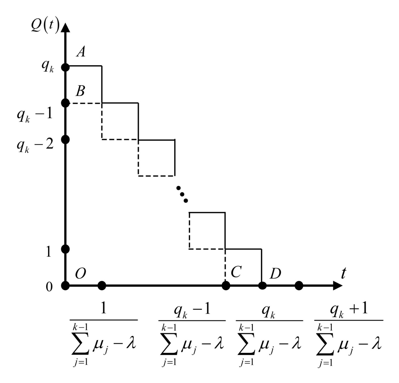
As it was mentioned above, the policy iteration algorithm has restrictions on dimension of the model, number of states, convergence in a heavy traffic case. In this section we derive a heuristic solution (HS) to estimate threshold levels $q_k$, $k=2,\dots ,K$, for the arbitrary K using a simple discrete fluid approximation $Q\left(t\right)-Q\left(t+\frac{1}{{\sum }_{j=1}^{k-1}{\mu }_j-\lambda }\right)=1$, $t=0,\frac{1}{{\sum }_{j=1}^{k-1}{\mu }_j-\lambda },\dots ,\frac{q_k-1}{{\sum }_{j=1}^{k-1}{\mu }_j-\lambda }$, for the queue length at time t, as illustrated in Figure 2.

We now explain how this fluid model can be employed for our aim. Assume that $q_k$ is an optimal threshold to allocate the customer to server k in state $(q_k-1,\underset{k-1}{\underbrace{1,\dots ,1}},\underset{K-k+1}{\underbrace{0,\dots ,0}})$, where the first $k-1$ servers are busy. Now we compare the queues of the system given initial state is $x_0=(q_k,\underset{k-1}{\underbrace{1,\dots ,1}},0,\underset{K-k}{\underbrace{0,\dots ,0}})$, where the kth server is not used for a new customer, and $y_0=(q_k-1,\underset{k-1}{\underbrace{1,\dots ,1}},1,\underset{K-k}{\underbrace{0,\dots ,0}})$, where the kth server is occupied by a waiting customer. It is assumed that the stability condition holds. In Figure 2, the queue lengths are labeled by $A=q_k$ and $B=q_k-1$. If the queue dynamics corresponded to the deterministic fluid, it would decrease at the rate ${\sum }_{j=1}^{k-1}{\mu }_j-\lambda$. When this rate is maintained until the queue is empty, it occurs respectively at points $D=\frac{q_k}{{\sum }_{j=1}^{k-1}{\mu }_j-\lambda }$ and $C=\frac{q_k-1}{{\sum }_{j=1}^{k-1}{\mu }_j-\lambda }$. The total holding times of customers in a queue with lengths $q_k$ and $q_k-1$ are equal obviously to the areas

$$\begin{array}{c}\hfill F_{AOD}=\frac{q_k(q_k+1)}{2}·\frac{1}{{\sum }_{j=1}^{k-1}{\mu }_j-\lambda }\mathrm{and}{F}_{BOC}=\frac{q_k(q_k-1)}{2}·\frac{1}{{\sum }_{j=1}^{k-1}{\mu }_j-\lambda }\end{array}$$

of triangles $AOD$ and $BOC$. The mean service time of customers by first $k-1$ busy servers until the queue is empty starting from state $x_0$ is equal to

$$q_k\left(\frac{1}{{\mu }_1}\frac{{\mu }_1}{{\sum }_{j=1}^{k-1}{\mu }_j}+\dots +\frac{1}{{\mu }_{k-1}}\frac{{\mu }_{k-1}}{{\sum }_{j=1}^{k-1}{\mu }_j}\right)=q_k\frac{k-1}{{\sum }_{j=1}^{k-1}{\mu }_j},$$

where $\frac{{\mu }_i}{{\sum }_{j=1}^{k-1}{\mu }_j}$ is a probability to be served by the ith server, and starting from state $y_0$—is equal to $(q_k-1)\frac{k-1}{{\sum }_{j=1}^{k-1}{\mu }_j}$.

According to a specified deterministic fluid schema we formulate

Proposition 2. 

The optimal thresholds $q_k$, $k=2,\dots ,K$, are defined by

$$\begin{array}{c}\hfill q_k\approx {\widehat{q}}_k=min\left\{{\widehat{q}}_{k-1},⌊\left(\sum _{j=1}^{k-1}{\mu }_j-\lambda \right)\left(\frac{1}{{\mu }_k}-\frac{k-1}{{\sum }_{j=1}^{k-1}{\mu }_j}\right)⌋+1\right\}.\end{array}$$

(11)

Proof. 

Denote by $V\left(x\right)$ the overall average holding time of customers until the system is empty given initial state is $x\in E$. The decision to perform the allocation to the kth server in state $(q_k-1,\underset{k-1}{\underbrace{1,\dots ,1}},\underset{K-k+1}{\underbrace{0,\dots ,0}})$ must lead to a reduction of the overall holding time under fluid schema, i.e.,

$$\begin{array}{c}\hfill V\left(x_0\right)-V\left(y_0\right)>0.\end{array}$$

(12)

where

$$\begin{array}{cc}\hfill V\left(x_0\right)& =F_{AOD}+q_k\frac{k-1}{{\sum }_{j=1}^{k-1}{\mu }_j}+V(0,\underset{k-1}{\underbrace{1,\dots ,1}},\underset{K-k+1}{\underbrace{0,\dots ,0}}),\hfill \end{array}$$

(13)

$$\begin{array}{cc}\hfill V\left(y_0\right)& =\frac{1}{{\mu }_k}+V(q_k-1,\underset{k-1}{\underbrace{1,\dots ,1}},0,\underset{K-k}{\underbrace{0,\dots ,0}})\hfill \\ \hfill & =\frac{1}{{\mu }_k}+F_{BOC}+(q_k-1)\frac{k-1}{{\sum }_{j=1}^{k-1}{\mu }_j}+V(0,\underset{k-1}{\underbrace{1,\dots ,1}},\underset{K-k+1}{\underbrace{0,\dots ,0}}).\hfill \end{array}$$

After substitution of (13) into (12) and some simple manipulations we get that the heuristic solution for the optimal threshold $q_k$ is defined then as the integer larger then 1 and the smallest integer (11) satisfying the inequality (12). □

Example 2. 

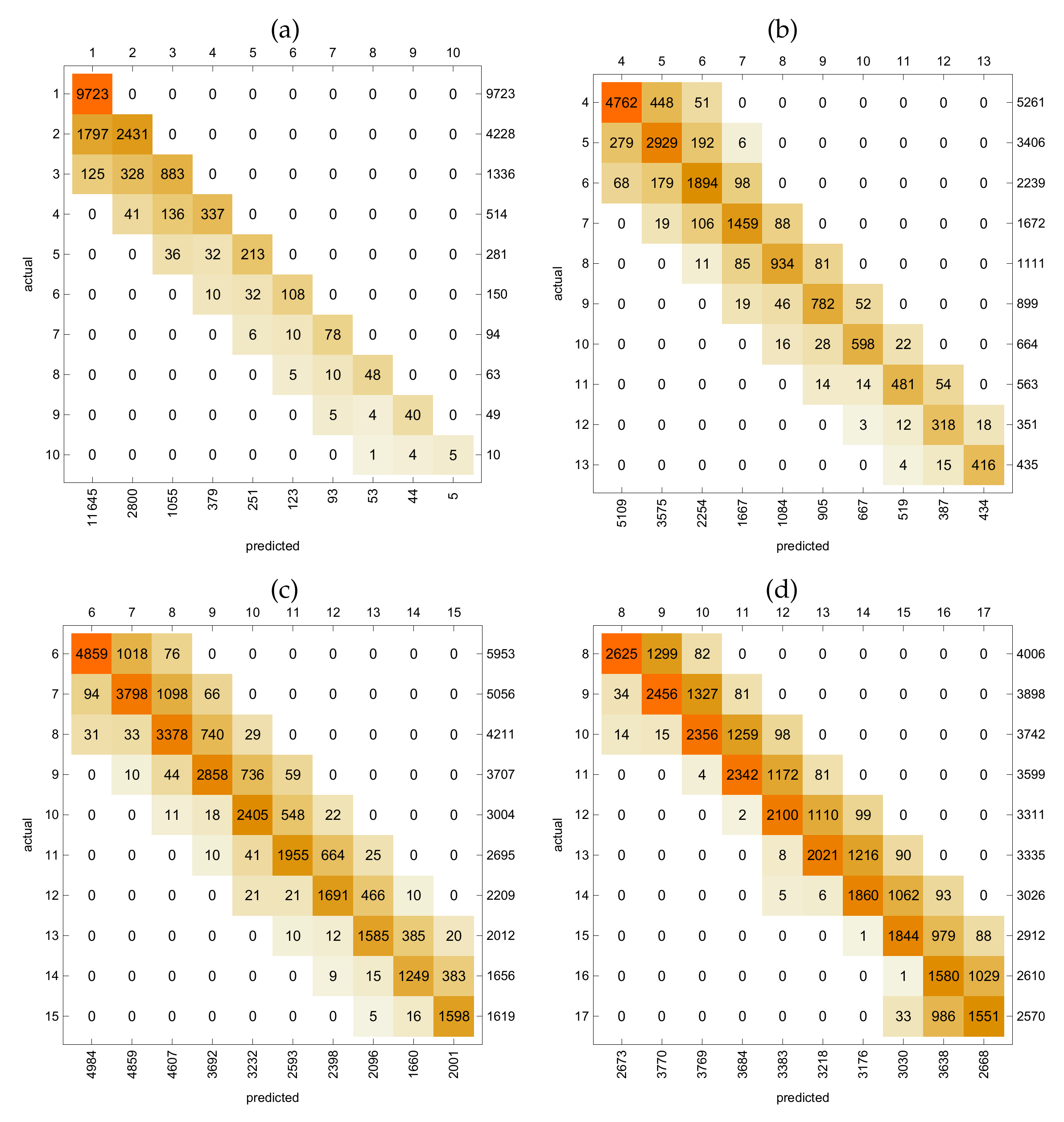
Consider a queueing system from previous example for $K=5$. We generate a data-set S in form of a list

$$\begin{array}{cc}\hfill & S=\hfill \\ \hfill & \left\{(\lambda ,{\mu }_1,\dots ,{\mu }_K)\to (q_2,\dots ,q_K):\lambda \in [1,45],{\mu }_1,\dots ,{\mu }_K\in [1,40],\lambda <\sum _{j=1}^K{\mu }_j,{\mu }_1\ge \dots \ge {\mu }_K\right\}.\hfill \end{array}$$

(14)

and evaluate with HS for the corresponding thresholds $q_k$, $k=1,\dots ,K$. Confusion matrices in Figure 3 visualize the performance of proposed heuristics respectively for the threshold levels $(q_2,q_3,q_4,q_5)$. Each row of these matrices represents the instances in a predicted value while each column represents the instances in an actual value. We notice the heavily diagonally dominant matrices that indicates a very good classification. This fact is confirmed also by overall accuracies. Such metrics describe the closeness of the heuristic measurements to a real threshold value and are calculated through the ratio of correct predictions to total predictions. Calculations of the overall accuracies as well as the accuracies for results with an acceptable deviation of threshold values by $\pm 1$ from the real value are summarized in

Table 1. Accuracy for prediction with heuristic solution (HS).

HS	${\mathit{q}}_2$	${\mathit{q}}_3$	${\mathit{q}}_4$	${\mathit{q}}_5$
Accuracy	0.8430	0.8778	0.7899	0.6282
Accuracy $\pm 1$	0.9861	0.9884	0.9871	0.9769

.

Example 3. 

Consider the queueing system $M/M/K$ with a different number of servers $K=2,3,\dots ,8$. Service rates take the values as given in

Table 2. Service rates ${\mu }_k$, $k=1,\dots ,K$.

	K	2	3	4	5	6	7	8
${\mu }_k$
${\mu }_1$		34	32	28	20	18	16	14
${\mu }_2$		1	2	4	8	8	8	6
${\mu }_3$		-	1	2	4	4	4	5
${\mu }_4$		-	-	1	2	2	3	4
${\mu }_5$		-	-	-	1	2	2	2
${\mu }_6$		-	-	-	-	1	1	2
${\mu }_7$		-	-	-	-	-	1	1
${\mu }_8$		-	-	-	-	-	-	1

.

Table 3. Threshold values $q_k$ and ${\widehat{q}}_k$, $k=2,\dots ,K$.

	K	2	3	4	5	6	7	8
$({\mathit{q}}_{\mathit{k}},{\widehat{\mathit{q}}}_{\mathit{k}})$
$(q_2,{\widehat{q}}_2)$		(24,24)	(11,11)	(5,4)	(1,1)	(1,1)	(1,1)	(1,1)
$(q_3,{\widehat{q}}_3)$		-	(23,23)	(10,10)	(4,4)	(3,3)	(3,3)	(2,2)
$(q_4,{\widehat{q}}_4)$		-	-	(22,22)	(9,9)	(8,9)	(4,5)	(2,2)
$(q_5,{\widehat{q}}_5)$		-	-	-	(21,22)	(8,9)	(8,8)	(7,7)
$(q_6,{\widehat{q}}_6)$		-	-	-	-	(20,21)	(19,20)	(7,8)
$(q_7,{\widehat{q}}_7)$		-	-	-	-	-	(19,20)	(19,19)
$(q_8,{\widehat{q}}_8)$		-	-	-	-	-	-	(19,20)

lists values of optimal thresholds $q_k$ and corresponding heuristic solutions ${\widehat{q}}_k$. As we see it, the maximum deviation of the optimal thresholds from the heuristic solution is 1 independently of the number of servers.

The large number of numerical experiments carried out using the policy-iteration algorithm and simulations allows us to conclude that deviations of certain thresholds by 1 have practically no effect on the value of the minimised function. Thus, we believe that the proposed heuristic solution is effective for an arbitrary number of servers.

4. Simple Bounds for the Optimal Mean Number of Customers in the System

As established in previous section, the estimation of the optimal threshold policy is possible by means of a simple heuristic solution. Nevertheless, with this knowledge it is quite complicated to calculate the optimal mean number of customers in the system with a high number of servers. A possible solution for this problem consists in construction a proper approximation of the original system with a preemption by an equivalent system without preemption. In this case a multidimensional Markov-chain can be described by an one-dimensional process. In this section we develop approximations for the low ${\overline{L}}_l$ and upper ${\overline{L}}_u$ bounds for the optimal gain function $g=\overline{L}$, ${\overline{L}}_l\le \overline{L}\le {\overline{L}}_u$.

To calculate the lower bound ${\overline{L}}_l$ we use a heterogeneous queueing system with a preemption and threshold-based control policy denoted by $S_l$ Further define by ${\left\{Y_l\left(t\right)\right\}}_{t\ge 0}$ the corresponding continuous-time Markov chain with a state space $E_l=\{y:y\in {\mathbb{N}}_0\}$ describing the number of customers in the system. The state transition diagram of this system is illustrated in Figure 4.

The optimal threshold levels $q_k$, $k=2,\dots ,K$ are calculated using the heuristic solution (11). Obviously, since the customer being served in a slower server can change it as the faster one becomes empty, the mean number of customers in the system must be lower comparing to an original queue. The steady-state probabilities ${\pi }_y={lim}_{t\to \infty }\mathbb{P}[Y_l\left(t\right)=y]$ obviously exist under the stability condition (2).

Proposition 3. 

The steady-state probabilities ${\pi }_y$ of the Markov chain ${\left\{Y_l\left(t\right)\right\}}_{t\ge 0}$ are given by

$$\begin{array}{cc}\hfill {\pi }_0& =[1+\sum _{y=1}^{q_2}{\left(\frac{\lambda }{{\mu }_1}\right)}^y+\sum _{k=3}^K\sum _{y=q_{k-1}}^{q_k}{\left(\frac{\lambda }{{\sum }_{j=1}^{k-1}{\mu }_j}\right)}^{y-q_{k-1}}·\prod _{i=1}^{k-2}{\left(\frac{\lambda }{{\sum }_{j=1}^i{\mu }_j}\right)}^{q_{i+1}-q_i}+\hfill \\ \hfill & +\prod _{i=1}^{K-1}{\left(\frac{\lambda }{{\sum }_{j=1}^i{\mu }_j}\right)}^{q_{i+1}-q_i}·\frac{\lambda }{{\sum }_{j=1}^K{\mu }_j-\lambda }{]}^{-1},\hfill \\ \hfill {\pi }_y& =\left\{\begin{array}{cc}{\pi }_0·{\left(\frac{\lambda }{{\mu }_1}\right)}^y,\hfill & 1\le y\le q_2\hfill \\ {\pi }_0·\prod _{i=1}^{k-2}{\left(\frac{\lambda }{{\sum }_{j=1}^i{\mu }_j}\right)}^{q_{i+1}-q_i}·{\left(\frac{\lambda }{{\sum }_{j=1}^{k-1}{\mu }_j}\right)}^{y-q_{k-1}},\hfill & q_{k-1}\le y\le q_k,3\le k\le K\hfill \\ {\pi }_0·\prod _{i=1}^{K-1}{\left(\frac{\lambda }{{\sum }_{j=1}^i{\mu }_j}\right)}^{q_{i+1}-q_i}·{\left(\frac{\lambda }{{\sum }_{j=1}^K{\mu }_j}\right)}^{y-q_K},\hfill & y\ge q_K+1\hfill \end{array}\right.\hfill \end{array}$$

Proof. 

The proposition follows directly from the properties of the ergodic birth-and-death process ${\left\{Y_l\left(t\right)\right\}}_{t\ge 0}$ [28]. □

From the probabilities ${\pi }_y$ it is possible to derive the performance measures of the system, e.g., the mean number of customers in the system $\overline{L}$ and the mean number of customers in the queue $\overline{Q}$.

Corollary 1. 

The mean number of customers in the system $S_l$ satisfies the relation

$$\begin{array}{c}\hfill {\overline{L}}_l=\sum _{y=0}^{\infty }{\pi }_y=\sum _{y=0}^{q_K}{\pi }_y+\frac{\lambda ({\sum }_{j=1}^K{\mu }_j+({\sum }_{j=1}^K{\mu }_j-\lambda )q_K)}{{({\sum }_{j=1}^K{\mu }_j-\lambda )}^2}{\pi }_{q_K}.\end{array}$$

(15)

The upper bound ${\overline{L}}_u$ for the optimal mean number of customers in the system can be obtained from an equivalent system under the FSF policy, see a state transition diagram in Figure 5, where $q_k=1$ for $k=1,\dots ,K$.

In this diagram the group of states with a certain number of busy servers are labeled by $(q,{\sum }_{j=1}^K{d}_j)$ according to the number of busy servers in a state. An analytical solution for the heterogeneous queueing system with the FSF policy, where all states of servers are taken into account, although possible, but it is limited by the number of servers in the system. The latter system can be approximated in turn by a heterogeneous system $S_u$ with a preemption with appropriate evaluated service rates $m_j$, $j=1,\dots ,K$. The dynamics of the system $S_u$ is described by the continuous-time Markov-chain $\left\{Y_u\left(t\right)\right\}$ with a state space $E_u=\{y:y\in {\mathbb{N}}_0\}$, where $Y_u\left(t\right)$ specifies the number of customers in the system at time t. The state transition diagram for this Markov-chain is presented in Figure 6.

The approximations for $m_j$ are based on the observation that the incentive to occupy the slower servers is getting higher as arrival rate increases.

Proposition 4. 

The service rates $m_j$, $j=1,\dots ,K-1$, of the queueing model ${\left\{Y_u\left(t\right)\right\}}_{t\ge 0}$ can be approximated by the following relations

$$\begin{array}{cc}\hfill & m_j=\left\{\begin{array}{cc}\sum _{i=1}^j{\mu }_i,\hfill & 0<\lambda \le \sum _{i=0}^{j-1}{\mu }_{K-i}\hfill \\ \sum _{i=0}^{j-1}\frac{{\mu }_{K-i}}{\lambda }\sum _{i=1}^j{\mu }_i+\sum _{i=1}^{k-j}\left(\frac{{\mu }_{K-i-j+1}}{\lambda }\sum _{n=1}^k{\mu }_{n+i}\right)\hfill & \\ +\left(1-\sum _{i=0}^{k-1}\frac{{\mu }_{K-i}}{\lambda }\right)\sum _{i=k-j+2}^{k+1}{\mu }_j,\hfill & \sum _{i=0}^{k-1}{\mu }_{K-i}<\lambda \le \sum _{i=0}^k{\mu }_{K-i},j\le k\le K-1,\hfill \end{array}\right.\hfill \\ \hfill & m_K=\sum _{i=1}^K{\mu }_i.\hfill \end{array}$$

(16)

Proof. 

For small arrival rate, e.g., $0<\lambda \le {\mu }_K$, most probably that only the first server which is the fastest one will be occupied and hence it will have the main contribution to the service rate $m_1$. When the values $\lambda$ are larger, e.g., ${\mu }_K<\lambda \le {\mu }_{K-1}+{\mu }_K$, the first server will have a contribution to ${\mu }_1$ with a probability $\frac{{\mu }_K}{\lambda }$ and the second server—with a complementary probability $(1-\frac{{\mu }_K}{\lambda })$. For larger values of $\lambda$, ${\mu }_{K-1}+{\mu }_K<\lambda \le {\mu }_{K-2}+{\mu }_{K-1}+{\mu }_K$ the first three servers will contribute to ${\mu }_1$ with probabilities $\frac{{\mu }_K}{\lambda }$, $\frac{{\mu }_{K-1}}{\lambda }$ and $\left(1-\frac{{\mu }_{K-1}+{\mu }_K}{\lambda }\right)$. Similarly we may derive the contribution of the servers larger values of $\lambda$ up to the condition ${\mu }_2+\dots ,+{\mu }_K<\lambda \le {\mu }_1+{\mu }_2+\dots +{\mu }_K$. To evaluate the contribution to the service rate $m_2$ in a state with two busy servers the same schema can be used. When $\lambda$ is small, $0<\lambda \le {\mu }_{K-1}+{\mu }_K$, the first two servers will form the service rate ${\mu }_2$. If ${\mu }_{K-1}+{\mu }_K<\lambda \le {\mu }_{K-2}+{\mu }_{K-1}+{\mu }_K$, the first three servers will have a contribution to ${\mu }_2$, the first and second servers contribute with a probability $\frac{{\mu }_1+{\mu }_2}{\lambda }$, the second and fourth–with a probability $\left(1-\frac{{\mu }_2+{\mu }_3}{\lambda }\right)$. When ${\sum }_{j=0}^2{\mu }_{K-j}<\lambda \le {\sum }_{j=0}^3{\mu }_{K-j}$, the four faster servers will serve the customers, the first and second server with probability $\frac{{\mu }_{K-1}+{\mu }_K}{\lambda }$, the second and third server with probability $\frac{{\mu }_3}{\lambda }$ and the third and fourth with probability $\left(1-\frac{{\mu }_{K-2}+{\mu }_{K-1}+{\mu }_K}{\lambda }\right)$. The procedure can be continued for larger values of $\lambda$ in a similar way as before. The proposed arguments can be summarized for all service rates $m_j$, $j=1,\dots ,K$, and the arbitrary number of servers K in form of the approximation (16). □

It can be verified that for any j the quotient $\frac{\lambda }{m_j}<1$ and $\lambda <m_K={\sum }_{j=1}^K{\mu }_j$. Now we can use the approximation (16) to derive the steady-state distribution.

Proposition 5. 

The steady-state probabilities ${\pi }_y$ of the Markov-chain ${\left\{Y_u\left(t\right)\right\}}_{t\ge 0}$ are given by

$$\begin{array}{cc}\hfill {\pi }_0& ={\left[1+\sum _{y=1}^{K-1}\frac{{\lambda }^y}{{\prod }_{j=1}^y{m}_j}+\frac{{\lambda }^{K+1}}{(m_K-\lambda ){\prod }_{j=1}^K{m}_j}\right]}^{-1},\hfill \\ \hfill {\pi }_y& =\left\{\begin{array}{cc}{\pi }_0·\frac{{\lambda }^y}{{\prod }_{j=1}^y{m}_j}\hfill & 1\le y\le K,\hfill \\ {\pi }_0·\frac{{\lambda }^y}{m_K^{y-K}{\prod }_{j=1}^K{m}_j}\hfill & y\ge K+1.\hfill \end{array}\right.\hfill \end{array}$$

Proof. 

The proposition follows from the properties of the ergodic birth-and-death process ${\left\{Y_u\left(t\right)\right\}}_{t\ge 0}$ [28]. □

Corollary 2. 

The mean number of customers in the system $S_u$ satisfies the relation

$$\begin{array}{c}\hfill {\overline{L}}_u=\sum _{y=0}^{\infty }{\pi }_y=\sum _{y=0}^K{\pi }_y+\frac{\lambda (m_K+(m_K-\lambda )K)}{{(m_K-\lambda )}^2}.\end{array}$$

(17)

Example 4. 

Consider the $M/M/K$ queueing system with a total service intensity equal to ${\sum }_{j=1}^K{\mu }_j=35$. Here we analyse the systems with different number of servers and their heterogeneity.

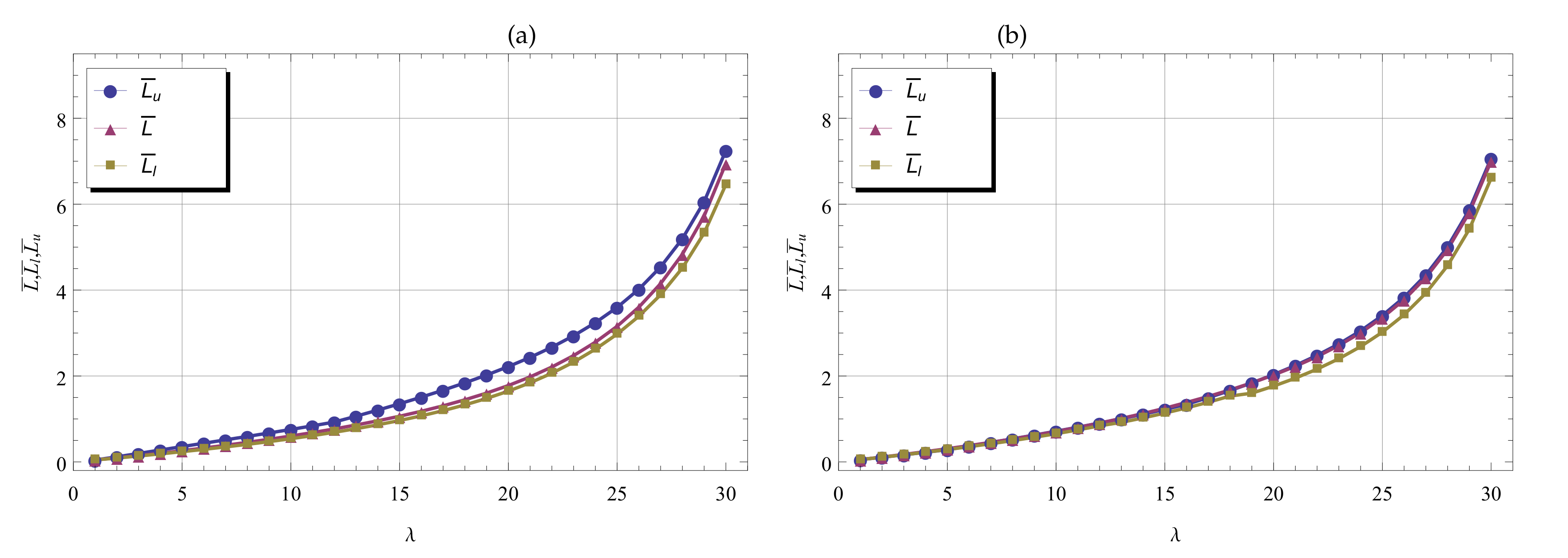
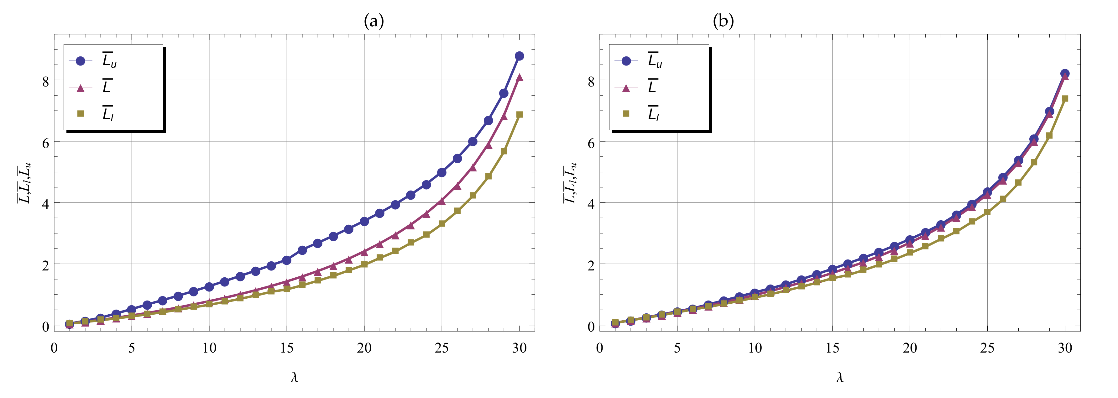
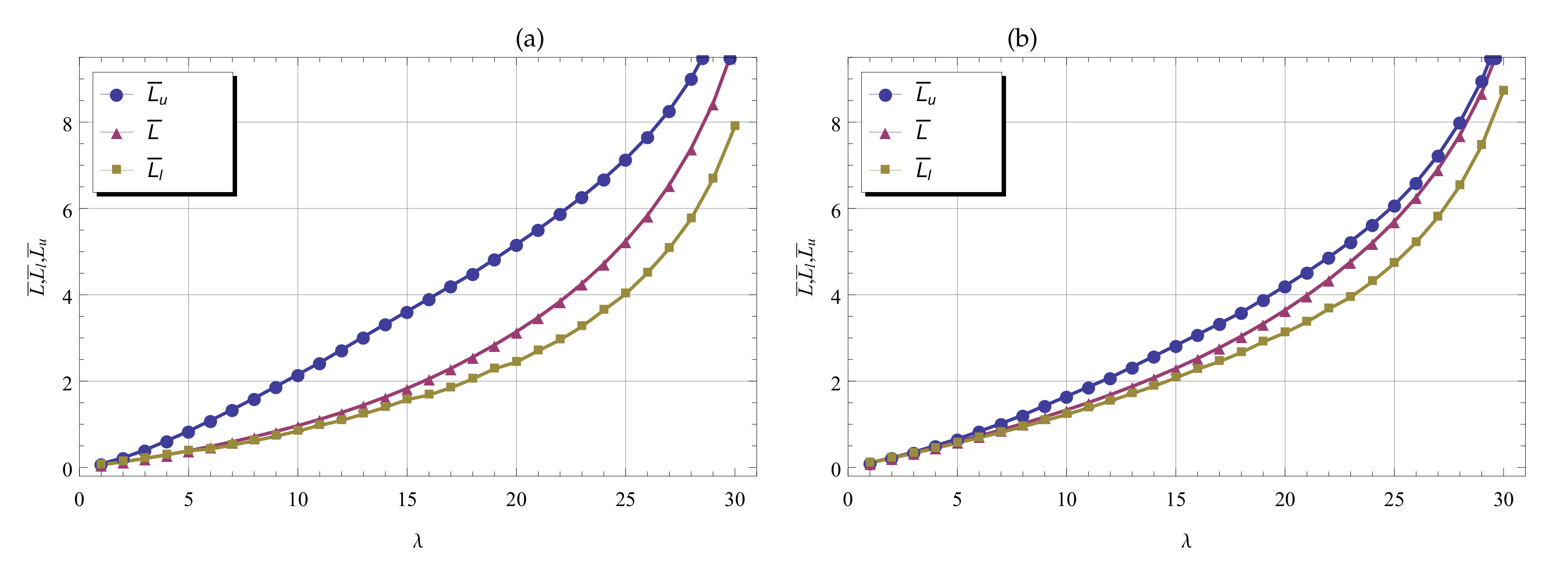
A Gini’s index $G\left(\mu \right)$, $0\le G\left(\mu \right)\le 1$, can be used to measure the inequality for individual data μ, see for details [29], and hence is quite appropriate as a metric for the heterogeneity of servers. This index can be obtained by computing the moments of the data set $\mu =\{{\mu }_K,{\mu }_{K-1},\dots ,{\mu }_1\}$ with ${\mu }_j$ sorted in increasing order,

$$\begin{array}{c}\hfill G\left(\mu \right)=\frac{2Cov[\mu ,n_K]}{K\overline{\mu }},\overline{\mu }=\frac{1}{K}\sum _{j=1}^K{\mu }_j,n_K=\{1,2,\dots ,K\}.\end{array}$$

The Gini’s index ranges from a minimum value of zero, when all individuals are equal, e.g., for the homogeneous servers $G\left(\mu \right)=0$, to a theoretical maximum of one when every individual except one has a value zero. Two different values of heterogeneity are studied within this example, namely $G\left(\mu \right)=0.63$ and $G\left(\mu \right)=0.40$. The corresponding values of service intensities for three types of systems with $K=3$, $K=5$ and $K=8$ are presented in

Table 4. Service intensities versus Gini’s index.

K	$\mathit{\mu }$	$\mathit{G}\left(\mathit{\mu }\right)$	K	$\mathit{\mu }$	$\mathit{G}\left(\mathit{\mu }\right)$
3	(1,11,23)	0.63	3	(5,11,19)	0.40
5	(1,2,4,8,20)	0.63	5	(2,4,6,10,13)	0.40
8	(0.5,1,1.5,2,2.5,3,7,17.5)	0.63	8	(1.5,1.5,2,3,4,6,8,9)	0.40

.

In Figure 7, Figure 8 and Figure 9 we display the values $\overline{L}$ with bounds ${\overline{L}}_l$ and ${\overline{L}}_u$ calculated respectively by the policy-iteration Algorithm 1 and by expressions (15) and (17) as functions of λ and number of servers $K=3,5,8$. The Gini’s index $G\left(\mu \right)=0.63$ in a figures labeled by (a) and $G\left(\mu \right)=0.40$—by (b). The curves in figures show, that the mean number of customers as well as the size of the gap between the lower and upper bounds increases with increasing values of K. As expected, the low and upper bounds must coincide with a mean value $\overline{L}$ for the system with homogeneous servers, where $G\left(\mu \right)=0$. Indeed, in figures with less heterogeneity of servers the curves for $\overline{L}$${\overline{L}}_u$ and ${\overline{L}}_l$ are getting closer, as the Gini’s index decreases. Moreover, we notice that the functions take similar values in a light traffic case when $\lambda <<{\sum }_{j=1}^K{\mu }_j$ and tend to the same values as the traffic becomes heavier, i.e., if $\lambda \to {\sum }_{j=1}^K{\mu }_j$.

5. Sensitivity Analysis of the Heuristic Solution to Changes in Distribution

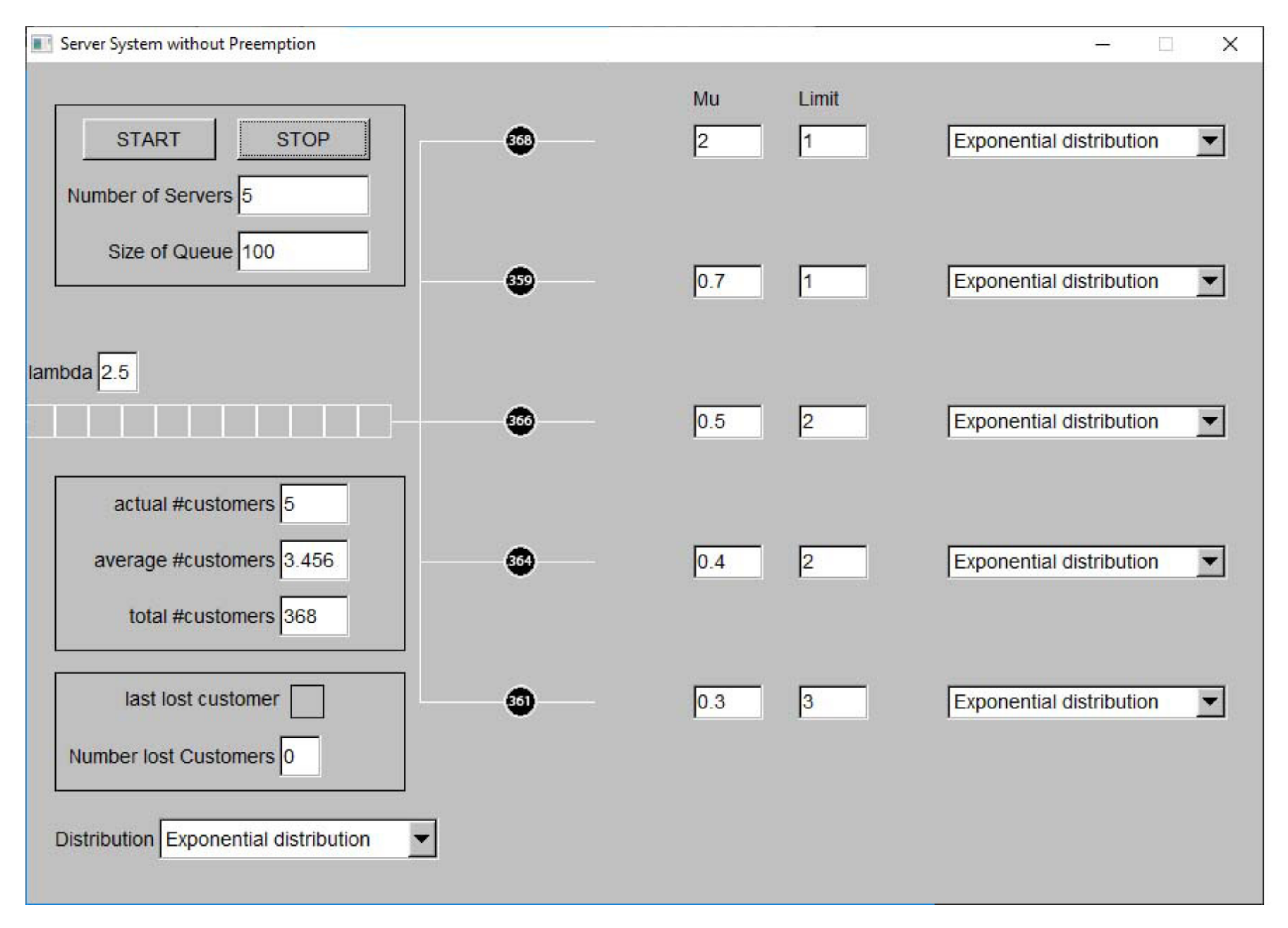
Another natural method to calculate the mean number of customers in the system and to check whether a certain policy leads to a reduction of this value is a simulation. This approach, while time-consuming, also makes it possible to examine the sensitivity of the optimal control policy f and the corresponding mean performance characteristics to changes in distribution types other than exponential. An implementation of a simulation model is shown in the Figure 10 bellow.

For this specific implementation it is possible to set the number of servers, the buffer capacity, threshold levels (limits), the arrival and service rates. The customers are indicated by a black circle, and are numbered accordingly to their arrival times. On the graphical interface there are also fields that show the actual amount of customers in the system, the average number and the total number of customers in the system including the already processed customers, the number of lost customers due to the truncated buffer capacity. The stability condition is taken into account and the buffer size is big enough so there should be hardly any lost customers. Hence the results with a truncated queue are comparable to systems with infinite queue lengths. Unfortunately, simulations are also unfit to solve systems with a large number of servers and states, as one would need to simulate a large number of different configurations with thousands of customers to get acceptable results. This fact further confirms the relevance of the results obtained in the previous sections.

The inter-arrival A and service times $B_j$, $j=1,2,\dots ,K$, of customers follow exponential, gamma, Pareto, log-normal and hyper-exponential distributions. To get comparable results the parameters of the distributions are chosen to have the same means $\mathbb{E}\left[A\right]=\frac{1}{\lambda }$, $\mathbb{E}\left[B_j\right]=\frac{1}{{\mu }_j}$, $j=1,2,\dots ,K$, and variances $\mathbb{V}\left[A\right]=\frac{1}{{\lambda }^2}$, $\mathbb{V}\left[B_j\right]=\frac{1}{{\mu }_j^2}$, $j=1,2,\dots ,K$, as the system driven by exponential distribution. For this purpose we use formulas describing the parameters in terms of the mean and variance given by Toth et al. [30]. The main goal of the simulation experiments consists in understanding weather the heuristic solution (11) for $\lambda =\frac{1}{\mathbb{E}\left[A\right]}$ and ${\mu }_j=\frac{1}{\mathbb{E}\left[B_j\right]}$ is insensitive to changes in forms of distributions.

Example 5. 

As a reference, we first simulate the system $M/M/5$ with an arrival rate $\lambda =25$, $({\mu }_1,{\mu }_2,{\mu }_3,{\mu }_4,{\mu }_5)=(20,8,4,2,1)$.

Table 5. Simulation results for the $M/M/5$ queueing system.

Exponential Distribution
Optimal Solution	Heuristic Solution	FSF	Lower Thresholds	Higher Thresholds
$q_2=1$	$q_2=1$	$q_2=1$	$q_2=1$	$q_2=2$
$q_3=2$	$q_3=2$	$q_3=1$	$q_3=1$	$q_3=3$
$q_4=4$	$q_4=3$	$q_4=1$	$q_4=2$	$q_4=4$
$q_5=9$	$q_5=8$	$q_5=1$	$q_5=7$	$q_5=9$
$L=4.082$	$L=4.189$	$L=4.860$	$L=4.213$	$L=4.674$

lists the mean number of customers in the system the optima, heuristic, FSF policies as well for other threshold policies with lower and higher values of thresholds.

We now simulate the systems like $GI/M/5$, $M/G/5$ as well as $GI/G/5$ with heterogeneous servers and threshold-based allocation policy where either the inter-arrival times, the service time or both follow one of the distributions mentioned above. For all the following simulation results we hereby want to find the mean number of customers in the system $\overline{L}$ for the policies specified in the preceding table for the markovian queueing system $M/M/5$.

Table 6. Simulation results for the $GI/M/5$, $M/G/5$ and $GI/G/5$ queueing systems.

gamma distribution
optimal solution	heuristic solution	FSF	lower thresholds	higher thresholds
GI/M/5: $L=4.491$	GI/M/5: $L=4.499$	GI/M/5: $L=5.230$	GI/M/5: $L=4.375$	GI/M/5: $L=5.002$
M/G/5: $L=4.527$	M/G/5: $L=4.646$	M/G/5: $L=5.011$	M/G/5: $L=4.742$	M/G/5: $L=5.223$
GI/G/5: $L=4.048$	GI/G/5: $L=4.154$	GI/G/5: $L=4.827$	GI/G/5: $L=4.352$	GI/G/5: $L=4.719$
Pareto distribution
optimal solution	heuristic solution	FSF	lower thresholds	higher thresholds
GI/M/5: $L=3.857$	GI/M/5: $L=3.958$	GI/M/5: $L=4.426$	GI/M/5: $L=3.889$	GI/M/5: $L=4.561$
M/G/5: $L=4.211$	M/G/5: $L=4.321$	M/G/5: $L=4.870$	M/G/5: $L=4.477$	M/G/5: $L=4.913$
GI/G/5: $L=3.385$	GI/G/5: $L=3.473$	GI/G/5: $L=3.837$	GI/G/5: $L=3.461$	GI/G/5: $L=4.051$
log-normal distribution
optimal solution	heuristic solution	FSF	lower thresholds	higher thresholds
GI/M/5: $L=4.366$	GI/M/5: $L=4.479$	GI/M/5: $L=4.911$	GI/M/5: $L=4.509$	GI/M/5: $L=5.037$
M/G/5: $L=4.429$	M/G/5: $L=4.545$	M/G/5: $L=4.870$	M/G/5: $L=4.824$	M/G/5: $L=5.139$
GI/G/5: $L=3.821$	GI/G/5: $L=3.921$	GI/G/5: $L=4.636$	GI/G/5: $L=3.975$	GI/G/5: $L=4.593$
hyper-exponential distribution
optimal solution	heuristic solution	FSF	lower thresholds	higher thresholds
GI/M/5: $L=4.043$	GI/M/5: $L=4.148$	GI/M/5: $L=4.771$	GI/M/5: $L=4.129$	GI/M/5: $L=4.645$
M/G/5: $L=4.024$	M/G/5: $L=4.129$	M/G/5: $L=4.707$	M/G/5: $L=4.167$	M/G/5: $L=4.801$
GI/G/5: $L=4.021$	GI/G/5: $L=4.126$	GI/G/5: $L=4.709$	GI/G/5: $L=4.233$	GI/G/5: $L=4.768$

provide a sensitivity and comparative analysis of the system performance obtained by employing different inter-arrival and service time distributions.

Of course, finding the optimal control policy through a simulation modelling is not an easy task. But in our example, we do not want to find the real values of the optimum thresholds, but rather to understand whether the optimum control and heuristic solution changes drastically when the distribution of the corresponding random values characterising the behaviour of a queueing system changes. Note that $\overline{L}$ for the optimal and heuristic policy takes always the values between those corresponding to the policies with lower and higher thresholds. The results of this example, as well as numerous other results carried out for systems with other parameters, show that while the absolute values of the mean number of customers vary as distributions change, the values of the optimal and heuristic thresholds are concentrated sufficiently close to the respective thresholds for markovian systems. Thus, we strongly believe, it is possible to use a heuristic solution with the replacement of exponential intensities by intensities of arbitrary distributions as a quasi-optimal solution in the problem of minimising the mean number of customers in the system with non-exponential inter-arrival and service time distributions.

6. Conclusions

The queueing systems with heterogeneous servers have many real applications. The optimal control policy which minimizes the mean number of customers in the system without preemption under certain assumptions belongs to a threshold policy. Classical methods, such as the solution of difference equations, matrix-analytic and dynamic-programming approach, have significant restrictions due to the dimension of the random processes involved. A heuristic solution is obtained for the optimal threshold levels in a system with an arbitrary number of servers. The simple lower and upper bounds for the minimal mean number of customers in the system are derived using one dimensional processes for the equivalent heterogeneous queues with a preemption. The gap between the bounds increases with increasing of the servers’ heterogeneity and the number of servers in the system. We have further conducted simulation to provide sensitivity analysis of the obtained HS to changes in inter-arrival and service time distributions. Simulation results showed that the optimal thresholds are likely to depend on the mean inter-arrival and service times and hence the proposed heuristic solution can be used as a quasi-optimal in systems with arbitrary distributions.