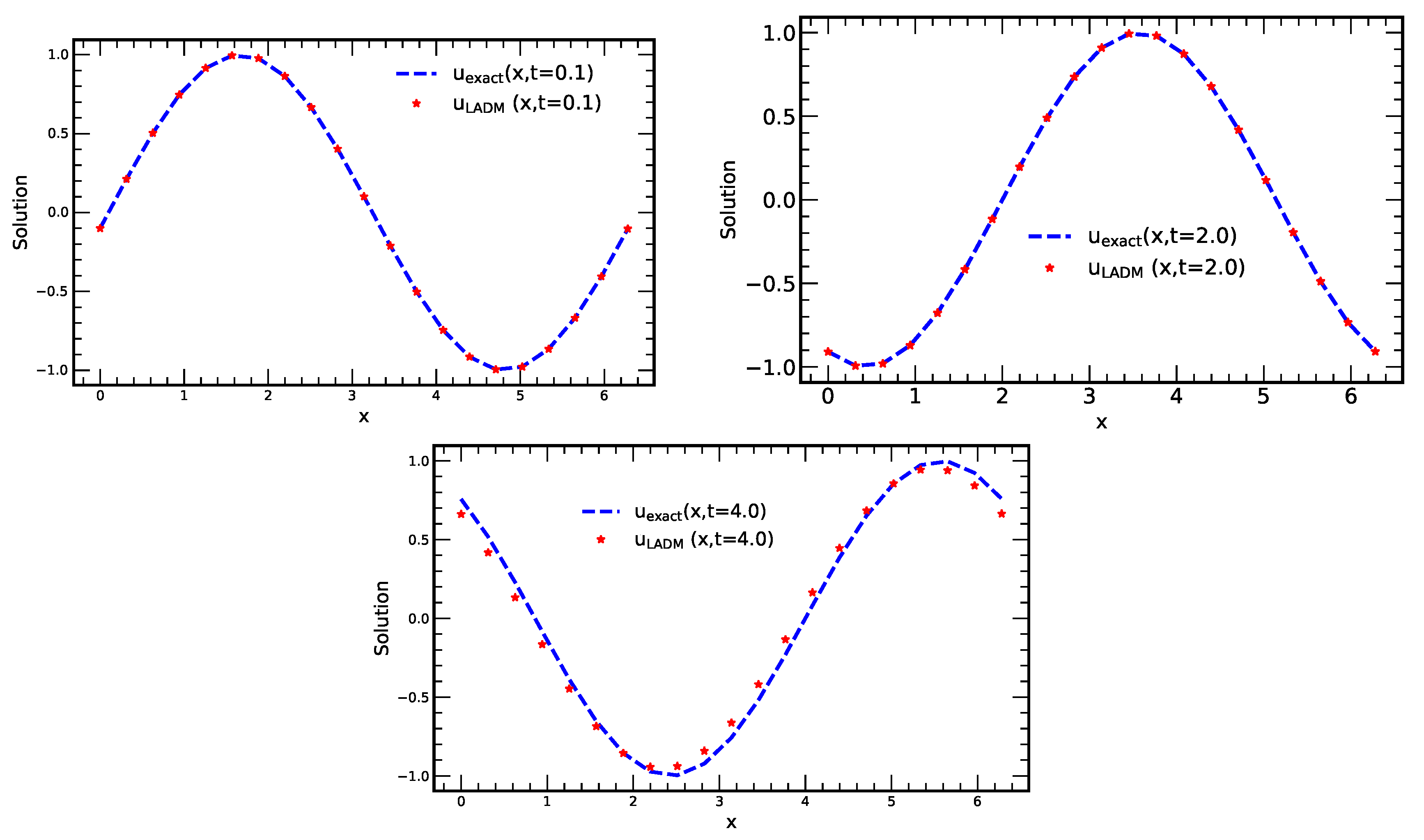
Figure 1.
Plots of exact solution and approximate solution using 10-terms of LADM, HPM, RDTM vs. x at times 0.1, 2.0 and 4.0. (The space interval used for these plots is ).
Figure 1.
Plots of exact solution and approximate solution using 10-terms of LADM, HPM, RDTM vs. x at times 0.1, 2.0 and 4.0. (The space interval used for these plots is ).
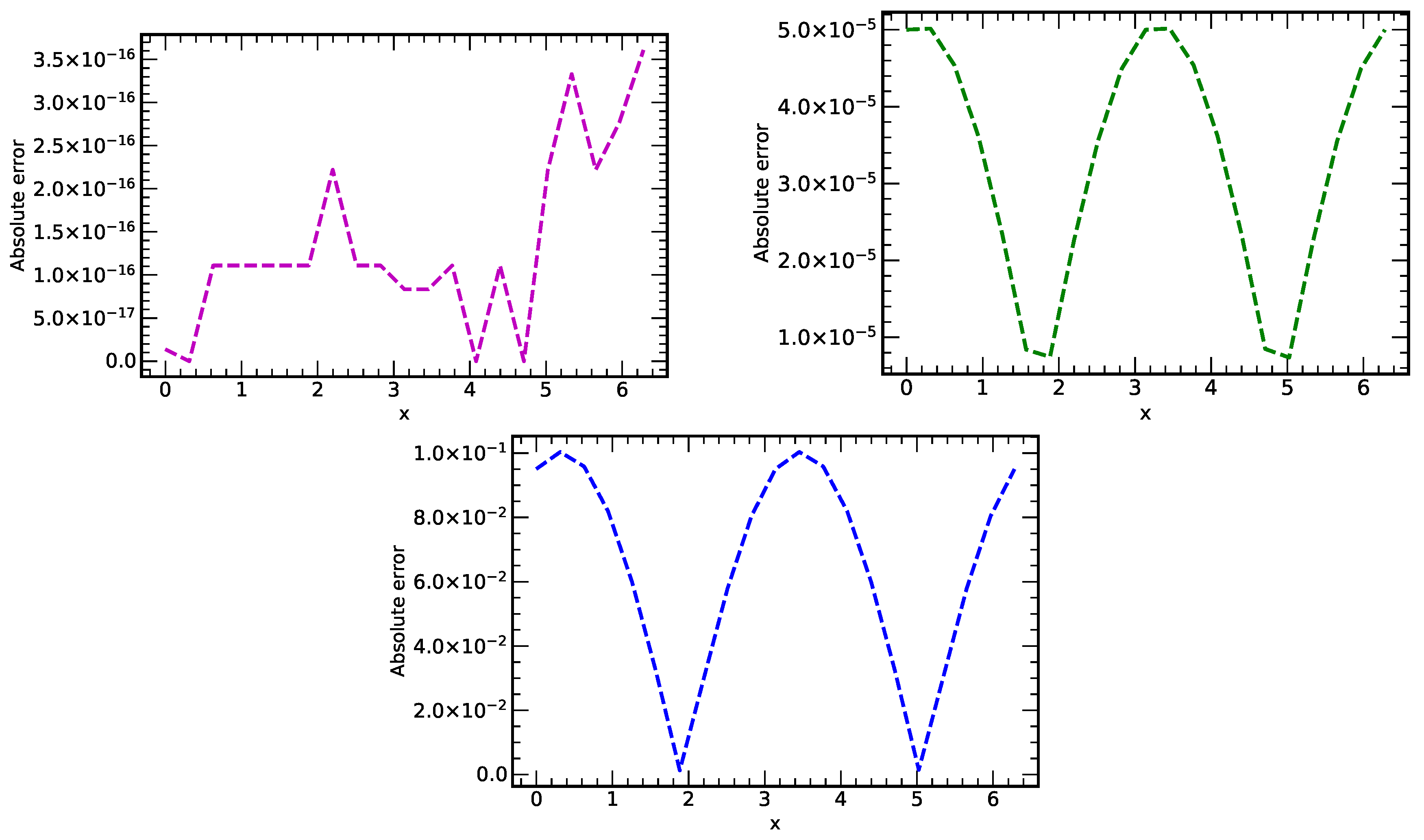
Figure 2.
Plots of absolute errors vs. x at different values of time () using the methods LADM, HPM and RDTM.
Figure 2.
Plots of absolute errors vs. x at different values of time () using the methods LADM, HPM and RDTM.
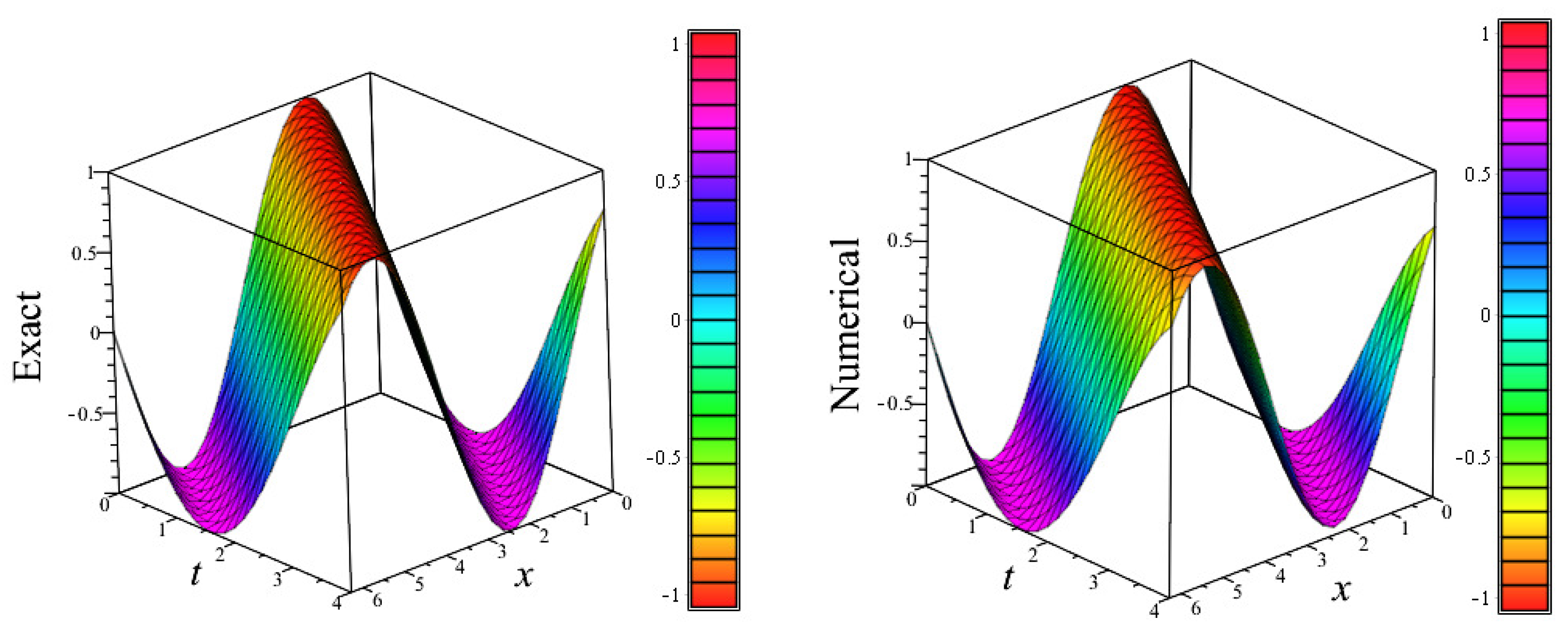
Figure 3.
3D plots of exact solution and approximate solution (using LADM, HPM, RDTM), vs. x vs. t, for numerical experiment 1.
Figure 3.
3D plots of exact solution and approximate solution (using LADM, HPM, RDTM), vs. x vs. t, for numerical experiment 1.
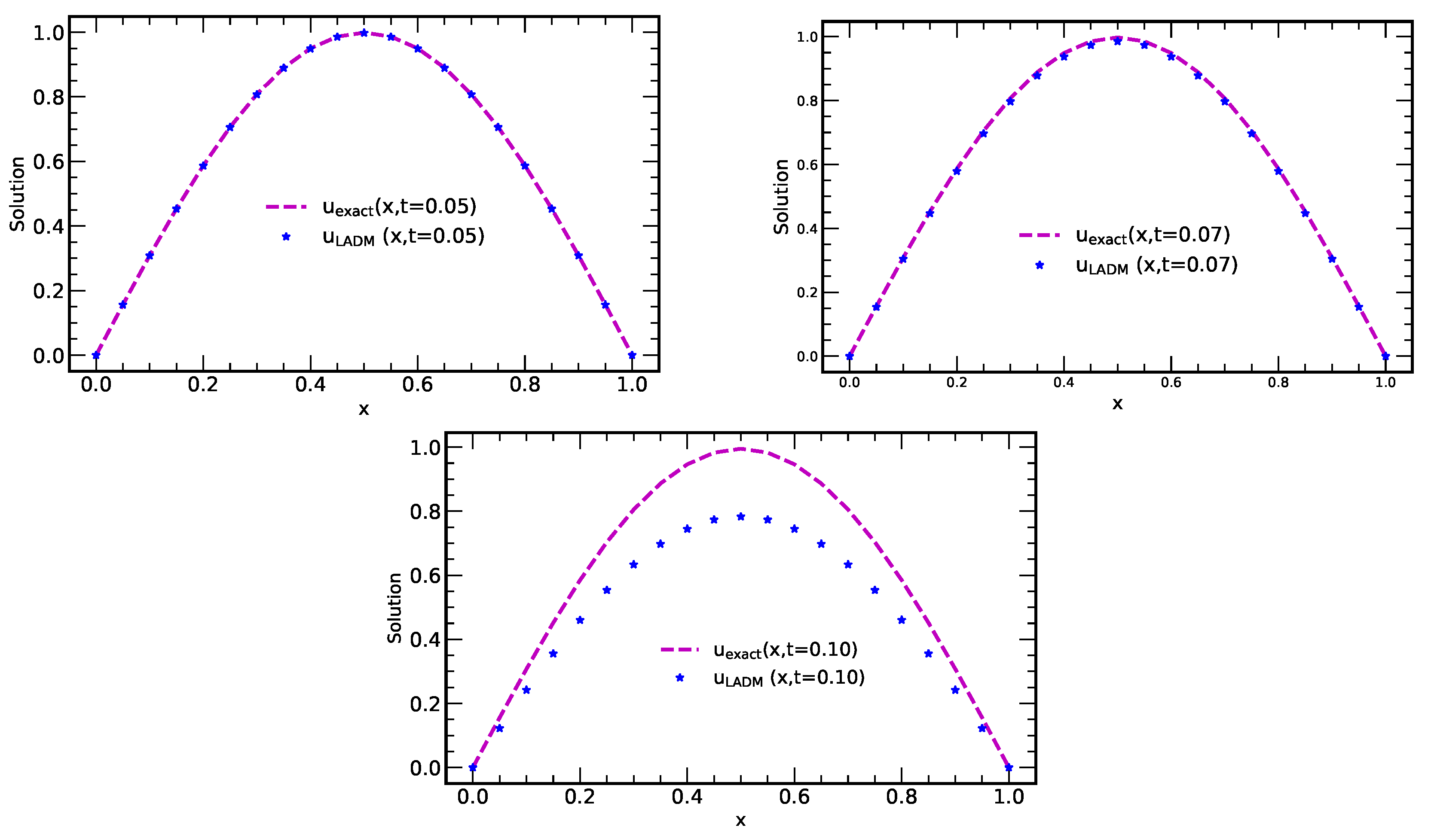
Figure 4.
Plots of exact solution and solution using LADM vs. x at different t-values, (for numerical experiment 2).
Figure 4.
Plots of exact solution and solution using LADM vs. x at different t-values, (for numerical experiment 2).
Figure 5.
Plots of absolute errors vs. x using 7-terms of LADM at different values of time ().
Figure 5.
Plots of absolute errors vs. x using 7-terms of LADM at different values of time ().
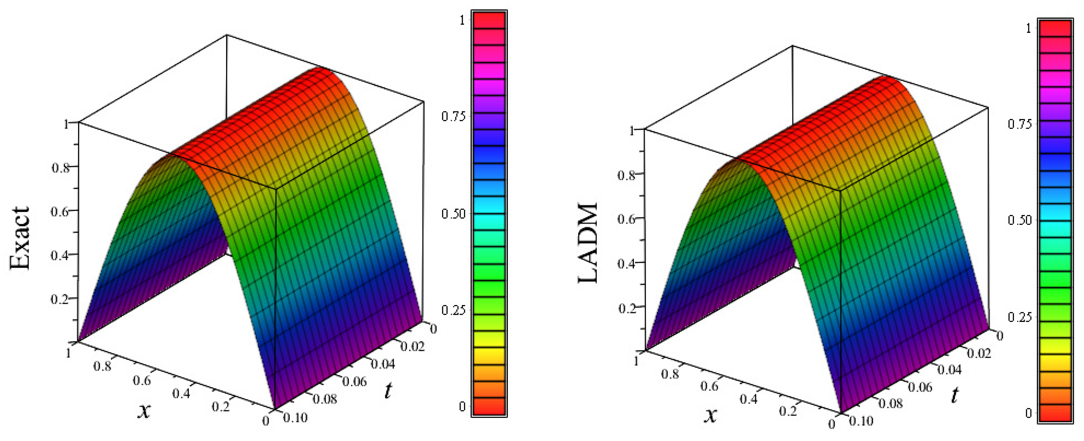
Figure 6.
3D plots of exact solution and approximate solution using LADM, vs. x vs. t, for numerical experiment 2.
Figure 6.
3D plots of exact solution and approximate solution using LADM, vs. x vs. t, for numerical experiment 2.
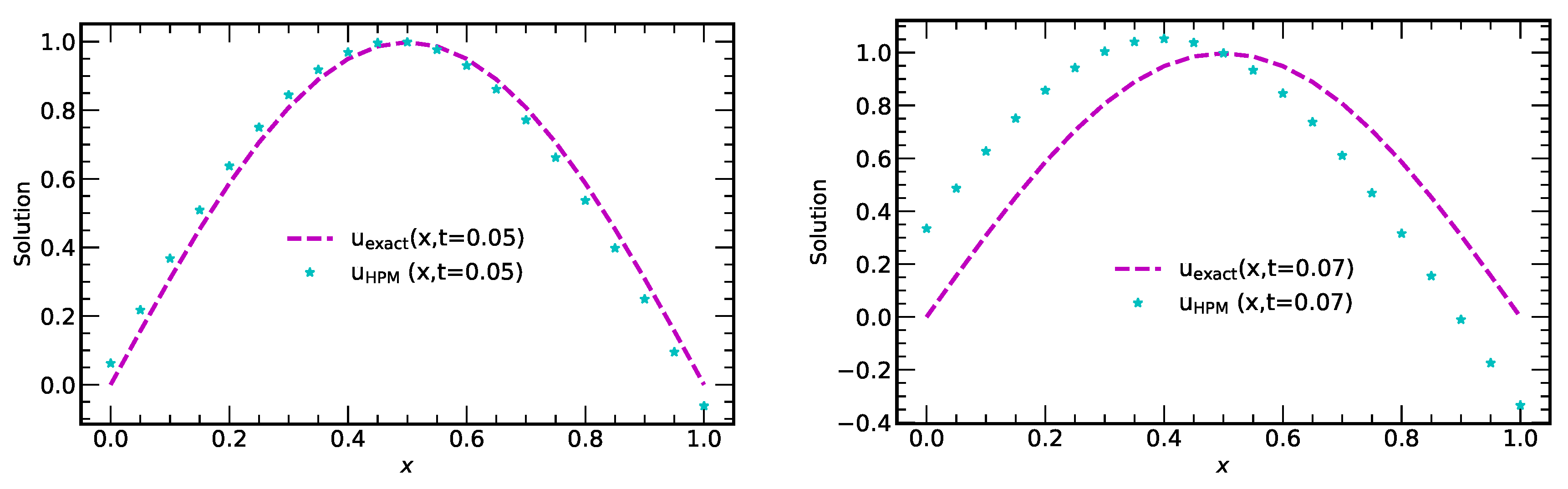
Figure 7.
Plots of exact solution and approximate solution using HPM at different t-values, (for numerical experiment 2).
Figure 7.
Plots of exact solution and approximate solution using HPM at different t-values, (for numerical experiment 2).
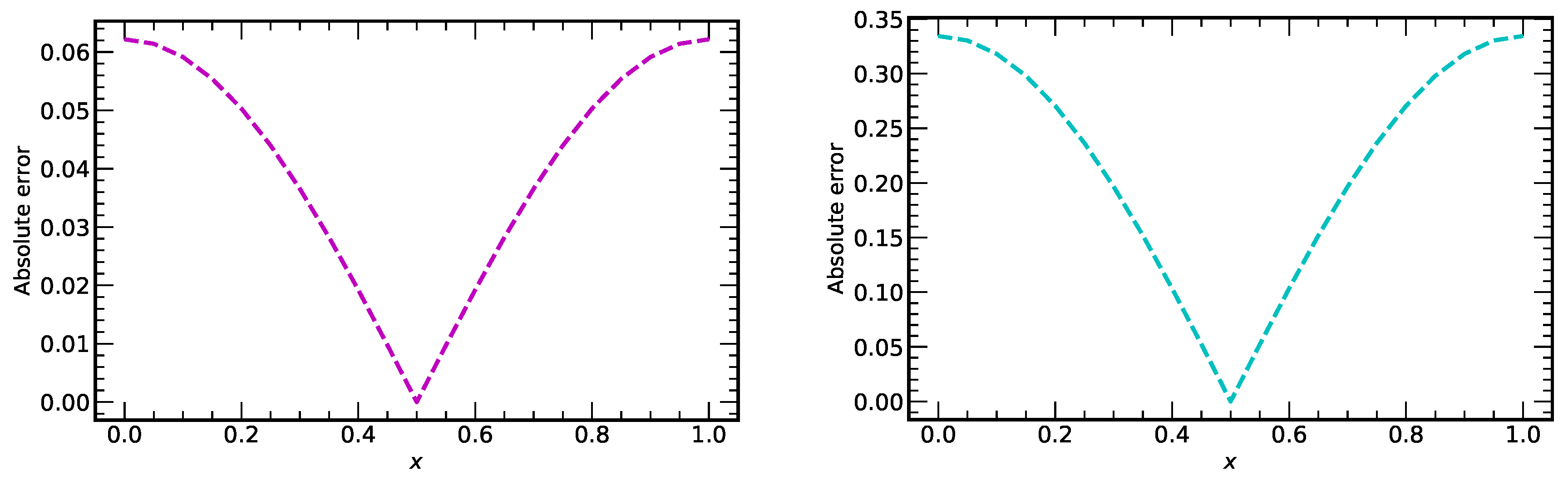
Figure 8.
Plots of absolute errors vs. x using 7-terms of HPM at different values of time ().
Figure 8.
Plots of absolute errors vs. x using 7-terms of HPM at different values of time ().
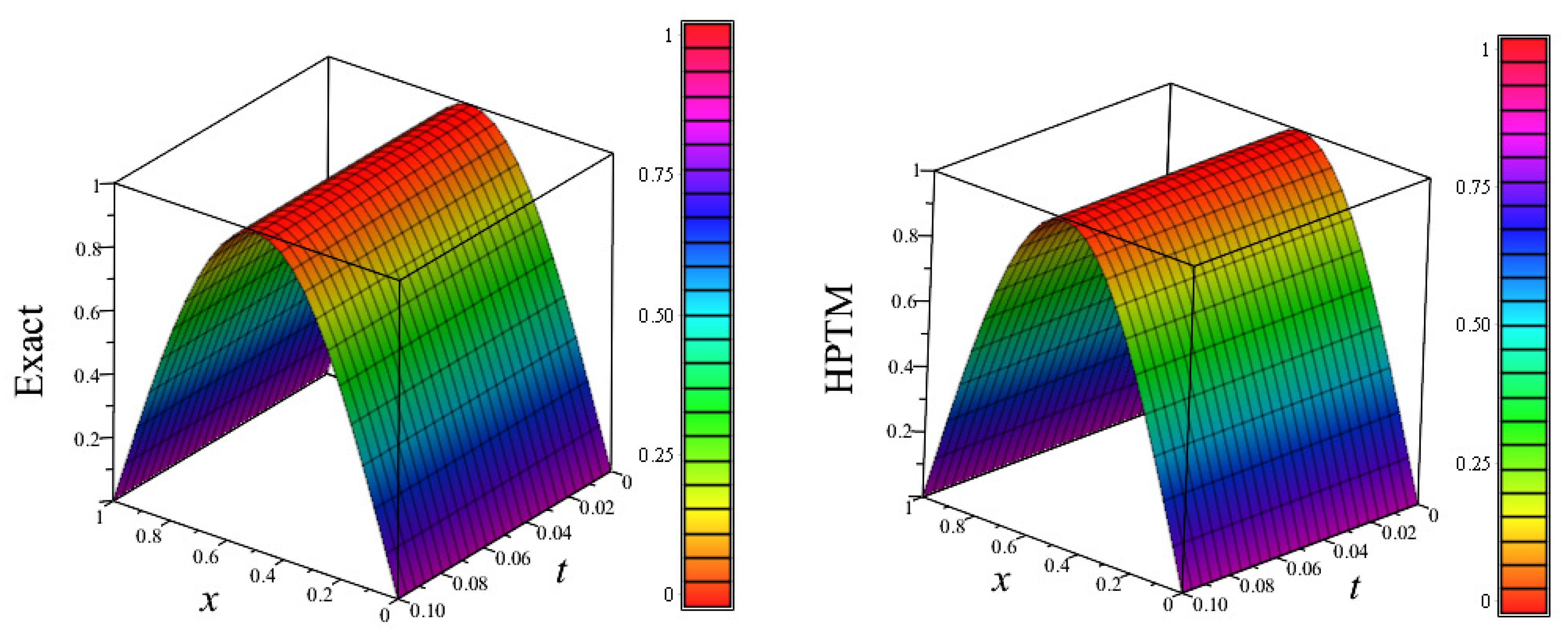
Figure 9.
3D plots of exact solution and approximate solution using HPTM, vs. x vs. t, for numerical experiment 2.
Figure 9.
3D plots of exact solution and approximate solution using HPTM, vs. x vs. t, for numerical experiment 2.
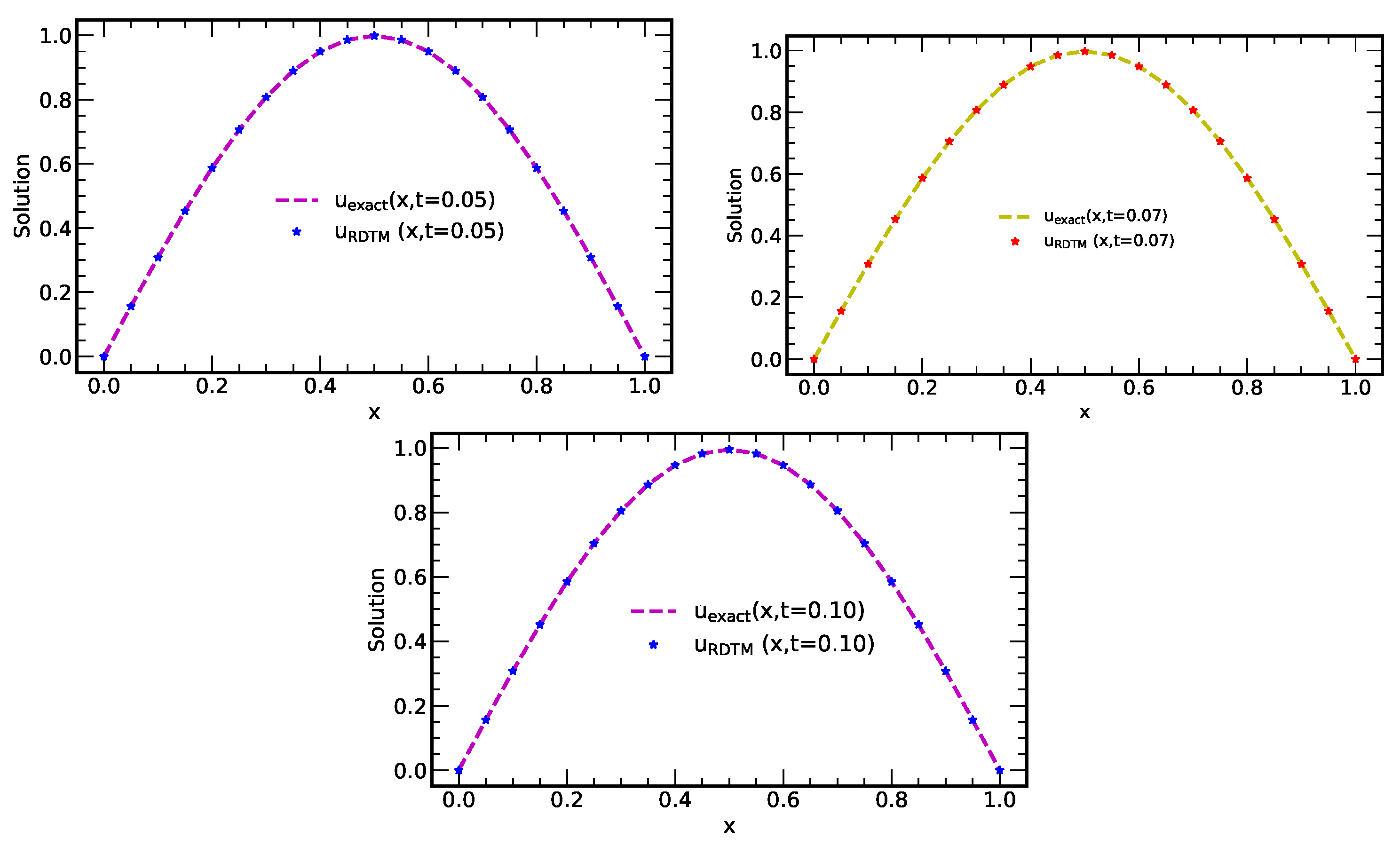
Figure 10.
Plots of exact solution and approximate solution using RDTM at (for numerical experiment 2).
Figure 10.
Plots of exact solution and approximate solution using RDTM at (for numerical experiment 2).
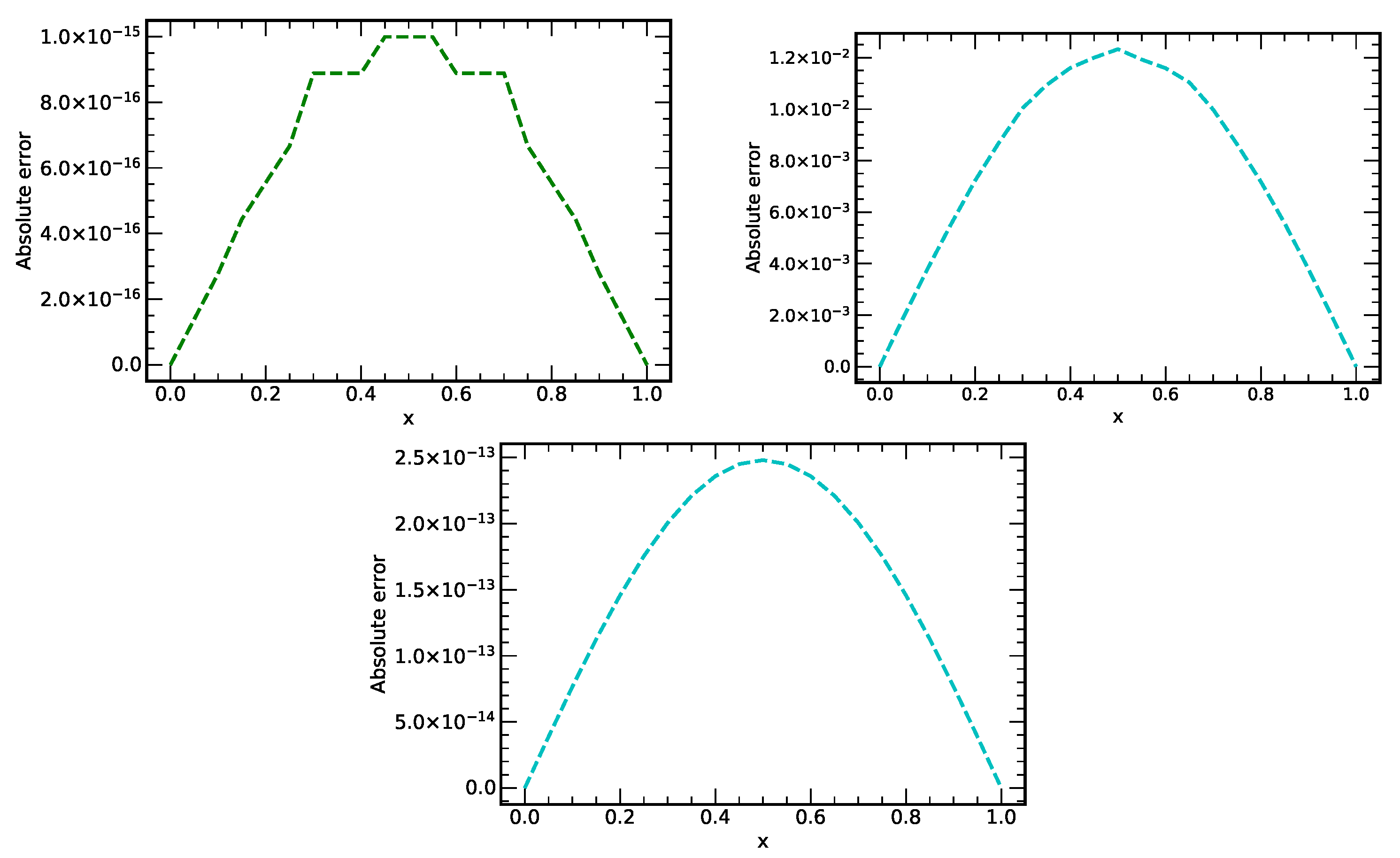
Figure 11.
Plots for absolute errors at different values of t ().
Figure 11.
Plots for absolute errors at different values of t ().
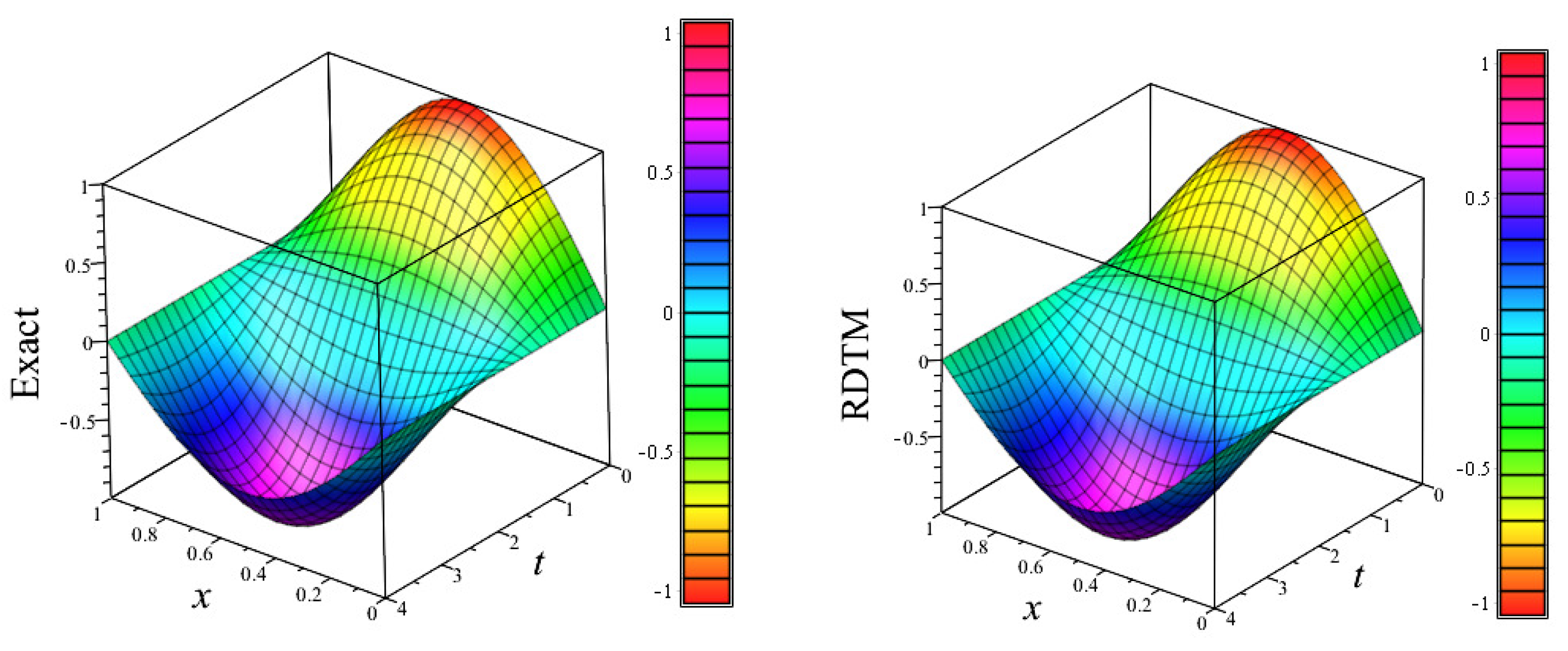
Figure 12.
3D plots of exact and approximate solution using RDTM, vs. x vs. t, for numerical experiment 2.
Figure 12.
3D plots of exact and approximate solution using RDTM, vs. x vs. t, for numerical experiment 2.
Figure 13.
Plots of exact solution and approximate solution using RDTM vs. x vs. y along and at .
Figure 13.
Plots of exact solution and approximate solution using RDTM vs. x vs. y along and at .
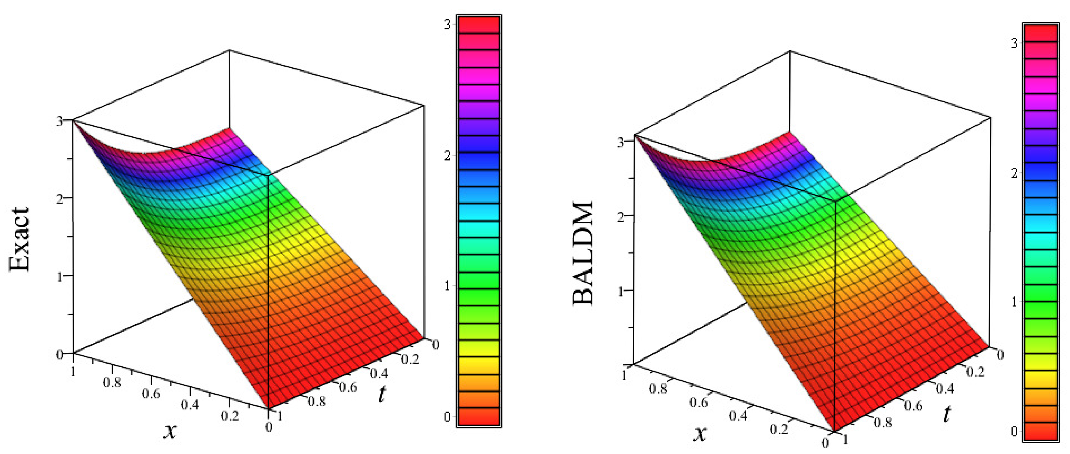
Figure 14.
3D plots of exact solution and sum of the first five approximate solution, , using BALDM, vs. x vs. t for numerical experiment 3.
Figure 14.
3D plots of exact solution and sum of the first five approximate solution, , using BALDM, vs. x vs. t for numerical experiment 3.
Figure 15.
Plots of exact solution and solution using BALDM at different t-values, (for numerical experiment 3).
Figure 15.
Plots of exact solution and solution using BALDM at different t-values, (for numerical experiment 3).
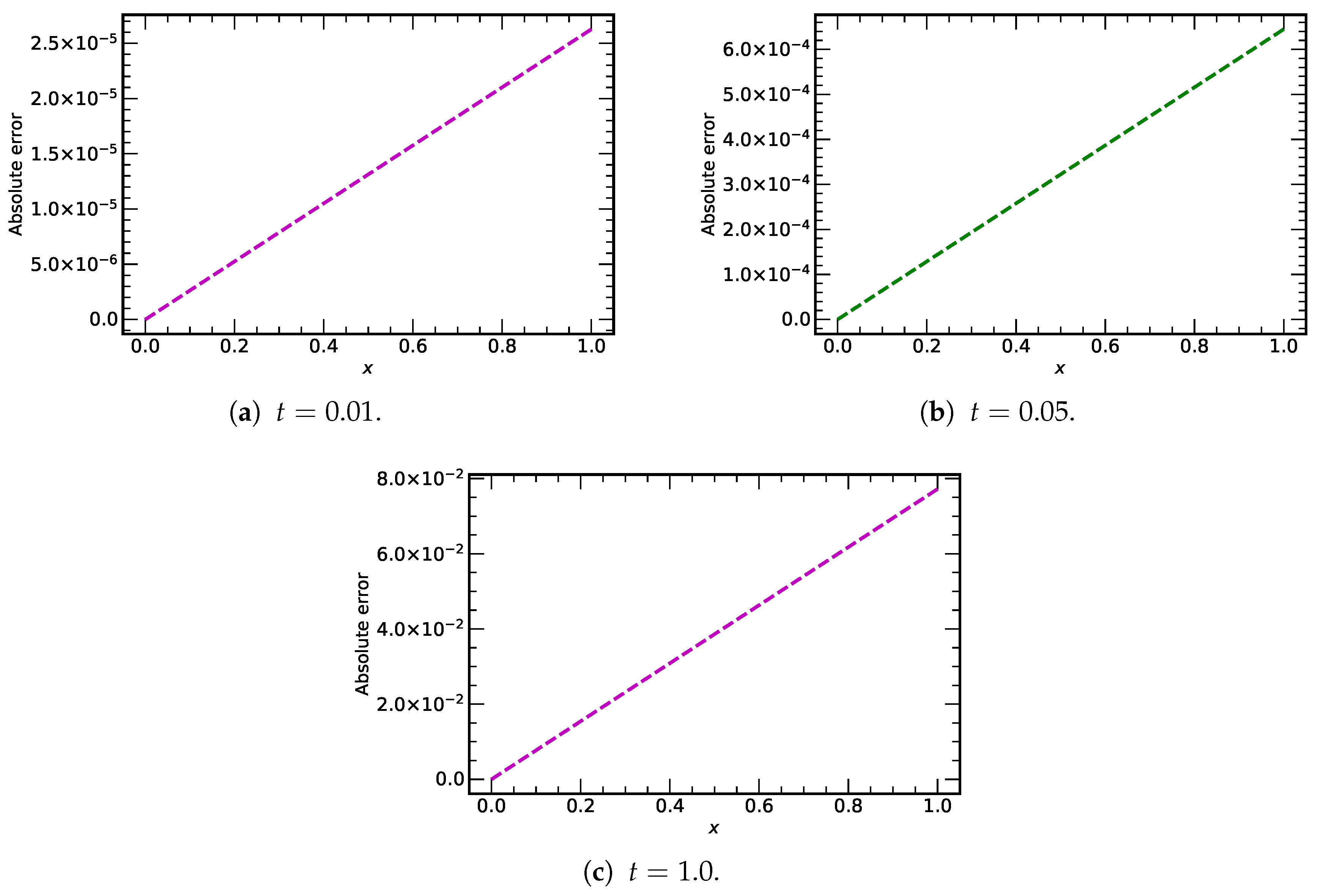
Figure 16.
Plots of absolute errors vs. x using 5-terms of BALDM at different values of time ().
Figure 16.
Plots of absolute errors vs. x using 5-terms of BALDM at different values of time ().
Table 1.
Absolute and relative errors at some values of x obtained at times 0.1, 2.0, 4.0 using 10-terms of LADM, HPM and RDTM for numerical experiment 1.
Table 1.
Absolute and relative errors at some values of x obtained at times 0.1, 2.0, 4.0 using 10-terms of LADM, HPM and RDTM for numerical experiment 1.
| t | Values of x | Exact Solution | Numerical Solution | Absolute Error | Relative Error |
|---|
| | 0.314 | 0.212370 | 0.212370 | 0.000000 | 0.000000 |
| | 0.628 | 0.503807 | 0.503807 | 1.110223 × | 2.203669 × |
| | 0.942 | 0.745977 | 0.745977 | 1.110223 × | 1.488281 × |
| | 1.256 | 0.915198 | 0.915198 | 1.110223 × | 1.213095 × |
| | 1.570 | 0.994924 | 0.994924 | 1.110223 × | 1.115887 × |
| | 1.884 | 0.977358 | 0.977358 | 1.110223 × | 1.135943 × |
| | 2.198 | 0.864217 | 0.864217 | 2.220446 × | 2.569314 × |
| | 2.512 | 0.666566 | 0.666566 | 1.110223 × | 1.665586 × |
| t = 0.1 | 2.826 | 0.403732 | 0.403732 | 1.110223 × | 2.749900 × |
| | 3.140 | 0.101418 | 0.101418 | 8.326673 × | 8.210252 × |
| | 3.454 | −0.210814 | −0.210814 | 8.326673 × | 3.949777 × |
| | 3.768 | −0.502430 | −0.502430 | 1.110223 × | 2.209705 × |
| | 4.082 | −0.744915 | −0.744915 | 0.000000 | 0.000000 |
| | 4.396 | −0.914555 | −0.914555 | 1.110223 × | 1.213948 × |
| | 4.710 | −0.994763 | −0.994763 | 0.000000 | 0.000000 |
| | 5.024 | −0.977694 | −0.977694 | 2.220446 × | 2.271106 × |
| | 5.338 | −0.865018 | −0.865018 | 3.330669 × | 3.850406 × |
| | 5.652 | −0.667752 | −0.667752 | 2.220446 × | 3.325253 × |
| | 5.966 | −0.405189 | −0.405189 | 2.775558 × | 6.850036 × |
| | 6.280 | −0.103002 | −0.103002 | 3.608225 × | 3.503053 × |
| | 0.314 | −0.993371 | −0.993422 | 5.015442 × | 5.048909 × |
| | 0.628 | −0.980305 | −0.980350 | 4.538846 × | 4.630034 × |
| | 0.942 | −0.871376 | −0.871412 | 3.618402 × | 4.152515 × |
| | 1.256 | −0.677236 | −0.677260 | 2.344120 × | 3.461303 × |
| | 1.570 | −0.416871 | −0.416879 | 8.406101 × | 2.016476 × |
| | 1.884 | −0.115740 | −0.115733 | 7.451020 × | 6.437721 × |
| | 2.198 | 0.196709 | 0.196731 | 2.257952 × | 1.147865 × |
| | 2.512 | 0.489922 | 0.489957 | 3.549999 × | 7.246054 × |
| t = 2.0 | 2.826 | 0.735226 | 0.735271 | 4.494898 × | 6.113628 × |
| | 3.140 | 0.908633 | 0.908683 | 5.000247 × | 5.503040 × |
| | 3.454 | 0.993187 | 0.993237 | 5.016629 × | 5.051041 × |
| | 3.768 | 0.980618 | 0.980664 | 4.542442 × | 4.632222 × |
| | 4.082 | 0.872156 | 0.872193 | 3.624056 × | 4.155283 × |
| | 4.396 | 0.678407 | 0.678431 | 2.351279 × | 3.465881 × |
| | 4.710 | 0.418318 | 0.418326 | 8.485738 × | 2.028538 × |
| | 5.024 | 0.117322 | 0.117314 | 7.371122 × | 6.282822 × |
| | 5.338 | −0.195147 | −0.195170 | 2.250717 × | 1.153344 × |
| | 5.652 | −0.488533 | −0.488568 | 3.544228 × | 7.254842 × |
| | 5.966 | −0.734146 | −0.734190 | 4.491153 × | 6.117524 × |
| | 6.280 | −0.907967 | −0.908017 | 4.998895 × | 5.505590 × |
| | 0.314 | 0.517911 | 0.417558 | 1.003528 × | 1.937646 × |
| | 0.628 | 0.228374 | 0.132556 | 9.581821 × | 4.195668 × |
| | 0.942 | −0.083495 | −0.165409 | 8.191365 × | 9.810567 × |
| | 1.256 | −0.387200 | −0.447199 | 5.999889 × | 1.549558 × |
| | 1.570 | −0.653041 | −0.685258 | 3.221691 × | 4.933369 × |
| | 1.884 | −0.855022 | −0.856306 | 1.284492 × | 1.502292 × |
| | 2.198 | −0.973391 | −0.943618 | 2.977354 × | 3.058743 × |
| | 2.512 | −0.996574 | −0.938654 | 5.792005 × | 5.811915 × |
| | 2.826 | −0.922304 | −0.841901 | 8.040265 × | 8.717588 × |
| t = 4.0 | 3.140 | −0.757843 | −0.662820 | 9.502279 × | 1.253859 × |
| | 3.454 | −0.519273 | −0.418922 | 1.003508 × | 1.932525 × |
| | 3.768 | −0.229924 | −0.134059 | 9.586562 × | 4.169441 × |
| | 4.082 | 0.081908 | 0.163914 | 8.200590 × | 0.1001194 × |
| | 4.396 | 0.385731 | 0.445858 | 6.012694 × | 1.558779 × |
| | 4.710 | 0.651834 | 0.684202 | 3.236825 × | 4.965722 × |
| | 5.024 | 0.854195 | 0.855639 | 1.444316 × | 1.690851 × |
| | 5.338 | 0.973025 | 0.943404 | 2.962086 × | 3.044203 × |
| | 5.652 | 0.996705 | 0.938915 | 5.778945 × | 5.798050 × |
| | 5.966 | 0.922918 | 0.842611 | 8.030689 × | 8.701410 × |
| | 6.280 | 0.758881 | 0.663909 | 9.497124 × | 1.251465 × |
Table 2.
Absolute and relative errors at some values of x obtained at times 0.05, 0.07, 0.10 using 7-terms of LADM (for numerical experiment 2).
Table 2.
Absolute and relative errors at some values of x obtained at times 0.05, 0.07, 0.10 using 7-terms of LADM (for numerical experiment 2).
| t | Values of x | Exact Solution | Numerical Solution | Absolute Error | Relative Error |
|---|
| | 0.050 | 0.156239 | 0.156108 | 1.306562 | 8.362586 |
| | 0.100 | 0.308631 | 0.308359 | 2.718451 | 8.808101 |
| | 0.150 | 0.453423 | 0.453017 | 4.062699 | 8.960062 |
| | 0.200 | 0.587051 | 0.586538 | 5.123988 | 8.728357 |
| | 0.250 | 0.706223 | 0.705581 | 6.422466 | 9.094104 |
| | 0.300 | 0.808006 | 0.807220 | 7.856065 | 9.722781 |
| | 0.350 | 0.889893 | 0.889146 | 7.466506 | 8.390341 |
| | 0.400 | 0.949868 | 0.948990 | 8.776868 | 9.240093 |
| | 0.450 | 0.986454 | 0.985657 | 7.967306 | 8.076713 |
| t = 0.05 | 0.500 | 0.998750 | 0.997896 | 8.544922 | 8.555614 |
| | 0.550 | 0.986454 | 0.985542 | 9.121347 | 9.246602 |
| | 0.600 | 0.949868 | 0.949037 | 8.314168 | 8.752972 |
| | 0.650 | 0.889893 | 0.889175 | 7.179544 | 8.067874 |
| | 0.700 | 0.808006 | 0.807327 | 6.791179 | 8.404863 |
| | 0.750 | 0.706223 | 0.705645 | 5.784568 | 8.190851 |
| | 0.800 | 0.587051 | 0.586586 | 4.644615 | 7.911779 |
| | 0.850 | 0.453423 | 0.452975 | 4.482223 | 9.885298 |
| | 0.900 | 0.308631 | 0.308353 | 2.775309 | 8.992326 |
| | 0.950 | 0.156239 | 0.156095 | 1.442404 | 9.232041 |
| | 1.000 | 0.000000 | 0.000000 | 1.386416 | 1.133511 |
| | 0.050 | 0.156051 | 0.154127 | 1.924276 | 1.233105 |
| | 0.100 | 0.308260 | 0.304473 | 3.786796 | 1.228441 |
| | 0.150 | 0.452879 | 0.447335 | 5.543939 | 1.224155 |
| | 0.200 | 0.586346 | 0.579125 | 7.220799 | 1.231492 |
| | 0.250 | 0.705375 | 0.696679 | 8.695814 | 1.232793 |
| | 0.300 | 0.807036 | 0.796997 | 1.003879 | 1.243910 |
| | 0.350 | 0.888824 | 0.877889 | 1.093497 | 1.230273 |
| | 0.400 | 0.948727 | 0.937126 | 1.160181 | 1.222881 |
| | 0.450 | 0.985269 | 0.973269 | 1.200080 | 1.218022 |
| t = 0.07 | 0.500 | 0.997551 | 0.985222 | 1.232910 | 1.235937 |
| | 0.550 | 0.985269 | 0.973345 | 1.192498 | 1.210326 |
| | 0.600 | 0.948727 | 0.937136 | 1.159155 | 1.221800 |
| | 0.650 | 0.888824 | 0.877787 | 1.103793 | 1.241857 |
| | 0.700 | 0.807036 | 0.797055 | 9.980618 | 1.236701 |
| | 0.750 | 0.705375 | 0.696737 | 8.638171 | 1.224621 |
| | 0.800 | 0.586346 | 0.579162 | 7.183557 | 1.225140 |
| | 0.850 | 0.452879 | 0.447314 | 5.564460 | 1.228687 |
| | 0.900 | 0.308260 | 0.304479 | 3.781563 | 1.226744 |
| | 0.950 | 0.156051 | 0.154130 | 1.920938 | 1.230966 |
| | 1.000 | 0.000000 | 0.000000 | 2.502025 | 2.048074 |
| | 0.050 | 0.155653 | 0.122508 | 3.314447 | 2.129383 |
| | 0.100 | 0.307473 | 0.242008 | 6.546499 | 2.129128 |
| | 0.150 | 0.451722 | 0.355480 | 9.624288 | 2.130576 |
| | 0.200 | 0.584849 | 0.460271 | 1.245775 | 2.130081 |
| | 0.250 | 0.703574 | 0.553690 | 1.498841 | 2.130323 |
| | 0.300 | 0.804975 | 0.633573 | 1.714020 | 2.129283 |
| | 0.350 | 0.886555 | 0.697687 | 1.888679 | 2.130357 |
| | 0.400 | 0.946305 | 0.744603 | 2.017019 | 2.131467 |
| | 0.450 | 0.982754 | 0.773581 | 2.091732 | 2.128439 |
| | 0.500 | 0.995004 | 0.783090 | 2.119141 | 2.129781 |
| t = 0.10 | 0.550 | 0.982754 | 0.773470 | 2.092838 | 2.129565 |
| | 0.600 | 0.946305 | 0.744687 | 2.016184 | 2.130586 |
| | 0.650 | 0.886555 | 0.697738 | 1.888175 | 2.129789 |
| | 0.700 | 0.804975 | 0.633604 | 1.713715 | 2.128904 |
| | 0.750 | 0.703574 | 0.553653 | 1.499208 | 2.130845 |
| | 0.800 | 0.584849 | 0.460341 | 1.245074 | 2.128883 |
| | 0.850 | 0.451722 | 0.355460 | 9.626242 | 2.131008 |
| | 0.900 | 0.307473 | 0.242018 | 6.545548 | 2.128819 |
| | 0.950 | 0.155653 | 0.122513 | 3.314019 | 2.129108 |
| | 1.000 | 0.000000 | 0.000000 | 1.001917 | 8.222354 |
Table 3.
Absolute and relative errors at some values of x obtained at times 0.05, 0.07 using 7-terms of HPM (for numerical experiment 2).
Table 3.
Absolute and relative errors at some values of x obtained at times 0.05, 0.07 using 7-terms of HPM (for numerical experiment 2).
| t | Values of x | Exact Solution | Numerical Solution | Absolute Error | Relative Error |
|---|
| | 0.050 | 0.156239 | 0.217665 | 6.142635 | 3.931564 |
| | 0.100 | 0.308631 | 0.367779 | 5.914842 | 1.916478 |
| | 0.150 | 0.453423 | 0.508837 | 5.541345 | 1.222113 |
| | 0.200 | 0.587051 | 0.637365 | 5.031456 | 8.570736 |
| | 0.250 | 0.706223 | 0.750199 | 4.397635 | 6.226977 |
| | 0.300 | 0.808006 | 0.844561 | 3.655552 | 4.524164 |
| | 0.350 | 0.889893 | 0.918127 | 2.823447 | 3.172794 |
| | 0.400 | 0.949868 | 0.969086 | 1.921845 | 2.023276 |
| | 0.450 | 0.986454 | 0.996183 | 9.728888 | 9.862485 |
| t = 0.05 | 0.500 | 0.998750 | 0.998750 | 9.331381 | 9.343057 |
| | 0.550 | 0.986454 | 0.976725 | 9.728769 | 9.862365 |
| | 0.600 | 0.949868 | 0.930650 | 1.921821 | 2.023251 |
| | 0.650 | 0.889893 | 0.861658 | 2.823459 | 3.172807 |
| | 0.700 | 0.808006 | 0.771450 | 3.655564 | 4.524179 |
| | 0.750 | 0.706223 | 0.662246 | 4.397659 | 6.227011 |
| | 0.800 | 0.587051 | 0.536737 | 5.031409 | 8.570655 |
| | 0.850 | 0.453423 | 0.398010 | 5.541309 | 1.222106 |
| | 0.900 | 0.308631 | 0.249483 | 5.914819 | 1.916471 |
| | 0.950 | 0.156239 | 0.094813 | 6.142611 | 3.931549 |
| | 0.050 | 0.156051 | 0.486414 | 3.303631 | 0.2117015 |
| | 0.100 | 0.308260 | 0.626371 | 3.181107 | 0.1031955 |
| | 0.150 | 0.452879 | 0.750904 | 2.980252 | 6.580686 |
| | 0.200 | 0.586346 | 0.856947 | 2.706008 | 4.615039 |
| | 0.250 | 0.705375 | 0.941889 | 2.365139 | 3.353024 |
| | 0.300 | 0.807036 | 1.003639 | 1.966030 | 2.436113 |
| | 0.350 | 0.888824 | 1.040676 | 1.518513 | 1.708451 |
| | 0.400 | 0.948727 | 1.052088 | 1.033602 | 1.089462 |
| | 0.450 | 0.985269 | 1.037594 | 5.232441 | 5.310670 |
| | 0.500 | 0.997551 | 0.997551 | 3.354171 | 3.362405 |
| | 0.550 | 0.985269 | 0.932945 | 5.232417 | 5.310645 |
| | 0.600 | 0.948727 | 0.845367 | 1.033602 | 1.089462 |
| t = 0.07 | 0.650 | 0.888824 | 0.736973 | 1.518512 | 1.708450 |
| | 0.700 | 0.807036 | 0.610433 | 1.966030 | 2.436113 |
| | 0.750 | 0.705375 | 0.468861 | 2.365137 | 3.353020 |
| | 0.800 | 0.586346 | 0.315745 | 2.706009 | 4.615041 |
| | 0.850 | 0.452879 | 0.154854 | 2.980249 | 6.580678 |
| | 0.900 | 0.308260 | −0.009850 | 3.181102 | 0.1031954 |
| | 0.950 | 0.156051 | −0.174312 | 3.303633 | 0.2117016 |
Table 4.
Transformed functions using RTDM.
Table 4.
Transformed functions using RTDM.
| Function | Transformed Function |
|---|
| |
| |
| |
| |
| (where ) |
| |
| |
Table 5.
Absolute and relative errors at some values of x obtained at times 0.05, 0.07, 0.10 using 7-terms of RDTM (for numerical experiment 2).
Table 5.
Absolute and relative errors at some values of x obtained at times 0.05, 0.07, 0.10 using 7-terms of RDTM (for numerical experiment 2).
| t | Values of x | Exact Solution | Numerical Solution | Absolute Error | Relative Error |
|---|
| | 0.050 | 0.156239 | 0.156239 | 1.387779 | 8.882412 |
| | 0.100 | 0.308631 | 0.308631 | 2.775558 | 8.993132 |
| | 0.150 | 0.453423 | 0.453423 | 4.440892 | 9.794145 |
| | 0.200 | 0.587051 | 0.587051 | 5.551115 | 9.455939 |
| | 0.250 | 0.706223 | 0.706223 | 6.661338 | 9.432343 |
| | 0.300 | 0.808006 | 0.808006 | 8.881784 | 1.099223 |
| | 0.350 | 0.889893 | 0.889893 | 8.881784 | 9.980733 |
| | 0.400 | 0.949868 | 0.949868 | 8.881784 | 9.350546 |
| | 0.450 | 0.986454 | 0.986454 | 9.992007 | 1.012922 |
| | 0.500 | 0.998750 | 0.998750 | 9.992007 | 1.000451 |
| t = 0.05 | 0.550 | 0.986454 | 0.986454 | 9.992007 | 1.012922 |
| | 0.600 | 0.949868 | 0.949868 | 8.881784 | 9.350546 |
| | 0.650 | 0.889893 | 0.889893 | 8.881784 | 9.980733 |
| | 0.700 | 0.808006 | 0.808006 | 8.881784 | 1.099223 |
| | 0.750 | 0.706223 | 0.706223 | 6.661338 | 9.432343 |
| | 0.800 | 0.587051 | 0.587051 | 5.551115 | 9.455939 |
| | 0.850 | 0.453423 | 0.453423 | 4.440892 | 9.794145 |
| | 0.900 | 0.308631 | 0.308631 | 2.775558 | 8.993132 |
| | 0.950 | 0.156239 | 0.156239 | 1.387779 | 8.882412 |
| | 1.000 | 0.000000 | 0.000000 | 1.232595 | 1.007750 |
| | 0.050 | 0.156051 | 0.156051 | 2.248202 | 1.440681 |
| | 0.100 | 0.308260 | 0.308260 | 4.385381 | 1.422623 |
| | 0.150 | 0.452879 | 0.452879 | 6.550316 | 1.446373 |
| | 0.200 | 0.586346 | 0.586346 | 8.437695 | 1.439031 |
| | 0.250 | 0.705375 | 0.705375 | 1.010303 | 1.432292 |
| | 0.300 | 0.807036 | 0.807036 | 1.165734 | 1.444464 |
| | 0.350 | 0.888824 | 0.888824 | 1.276756 | 1.436455 |
| | 0.400 | 0.948727 | 0.948727 | 1.365574 | 1.439375 |
| | 0.450 | 0.985269 | 0.985269 | 1.409983 | 1.431064 |
| t = 0.07 | 0.500 | 0.997551 | 0.997551 | 1.432188 | 1.435704 |
| | 0.550 | 0.985269 | 0.985269 | 1.409983 | 1.431064 |
| | 0.600 | 0.948727 | 0.948727 | 1.365574 | 1.439375 |
| | 0.650 | 0.888824 | 0.888824 | 1.276756 | 1.436455 |
| | 0.700 | 0.807036 | 0.807036 | 1.165734 | 1.444464 |
| | 0.750 | 0.705375 | 0.705375 | 1.010303 | 1.432292 |
| | 0.800 | 0.586346 | 0.586346 | 8.437695 | 1.439031 |
| | 0.850 | 0.452879 | 0.452879 | 6.550316 | 1.446373 |
| | 0.900 | 0.308260 | 0.308260 | 4.385381 | 1.422623 |
| | 0.950 | 0.156051 | 0.156051 | 2.248202 | 1.440681 |
| | 1.000 | 0.000000 | 0.000000 | 1.750285 | 1.432725 |
| | 0.050 | 0.155653 | 0.155653 | 3.880229 | 2.492873 |
| | 0.100 | 0.307473 | 0.307473 | 7.666090 | 2.493255 |
| | 0.150 | 0.451722 | 0.451722 | 1.126321 | 2.493392 |
| | 0.200 | 0.584849 | 0.584849 | 1.457723 | 2.492478 |
| | 0.250 | 0.703574 | 0.703574 | 1.754152 | 2.493202 |
| | 0.300 | 0.804975 | 0.804975 | 2.006173 | 2.492217 |
| | 0.350 | 0.886555 | 0.886555 | 2.210454 | 2.493307 |
| | 0.400 | 0.946305 | 0.946305 | 2.359224 | 2.493090 |
| | 0.450 | 0.982754 | 0.982754 | 2.450262 | 2.493261 |
| t = 0.10 | 0.500 | 0.995004 | 0.995004 | 2.480238 | 2.492691 |
| | 0.550 | 0.982754 | 0.982754 | 2.450262 | 2.493261 |
| | 0.600 | 0.946305 | 0.946305 | 2.359224 | 2.493090 |
| | 0.650 | 0.886555 | 0.886555 | 2.210454 | 2.493307 |
| | 0.700 | 0.804975 | 0.804975 | 2.006173 | 2.492217 |
| | 0.750 | 0.703574 | 0.703574 | 1.754152 | 2.493202 |
| | 0.800 | 0.584849 | 0.584849 | 1.457723 | 2.492478 |
| | 0.850 | 0.451722 | 0.451722 | 1.126321 | 2.493392 |
| | 0.900 | 0.307473 | 0.307473 | 7.666090 | 2.493255 |
| | 0.950 | 0.155653 | 0.155653 | 3.880229 | 2.492873 |
| | 1.000 | 0.000000 | 0.000000 | 3.037114 | 2.492444 |
Table 6.
Comparison between the exact solution and five-term approximation solution via RDTM.
Table 6.
Comparison between the exact solution and five-term approximation solution via RDTM.
| z | | | Absolute Error | Relative Error |
|---|
| | 0.1 | 0.27070402 | 0.27070489 | 8.72219677 × | 3.22204181 |
| (0.1, 0.1) | 0.5 | 0.46688742 | 0.46688893 | 1.50433080 × | 3.22204181 × |
| | 0.9 | 0.06765654 | 0.06765675 | 2.17992187 × | 3.22204181 × |
| | 0.1 | 0.46688742 | 0.46688893 | 1.50433080 × | 3.22204181 × |
| (0.5, 0.5) | 0.5 | 0.06765654 | 0.06765675 | 2.17992187 × | 3.22204181 × |
| | 0.9 | −0.41785568 | −0.41785703 | 1.34634848 × | 3.22204181 × |
| | 0.1 | 0.06765654 | 0.06765675 | 2.17992187 × | 3.22204181 × |
| (0.9, 0.9) | 0.5 | −0.41785568 | −0.41785703 | 1.34634848 × | 3.22204181 × |
| | 0.9 | −0.37048303 | −0.37048422 | 1.19371181 × | 3.22204181 × |
Table 7.
Absolute and relative errors at some values of x obtained at times 0.01, 0.05, 1.0 using of BALDM (for numerical experiment 3).
Table 7.
Absolute and relative errors at some values of x obtained at times 0.01, 0.05, 1.0 using of BALDM (for numerical experiment 3).
| t | Values of x | Exact Solution | Numerical Solution | Absolute Error | Relative Error |
|---|
| | 0.050 | 0.100000 | 0.100001 | 1.313616 | 1.313616 |
| | 0.100 | 0.200000 | 0.200003 | 2.627233 | 1.313616 |
| | 0.150 | 0.300000 | 0.300004 | 3.940849 | 1.313616 |
| | 0.200 | 0.400000 | 0.400005 | 5.254466 | 1.313616 |
| | 0.250 | 0.500000 | 0.500007 | 6.568082 | 1.313616 |
| | 0.300 | 0.600000 | 0.600008 | 7.881698 | 1.313616 |
| | 0.350 | 0.700000 | 0.700010 | 9.195315 | 1.313616 |
| | 0.400 | 0.800000 | 0.800011 | 1.050893 | 1.313616 |
| t = 0.01 | 0.450 | 0.900000 | 0.900012 | 1.182255 | 1.313616 |
| | 0.500 | 1.000001 | 1.000014 | 1.313616 | 1.313616 |
| | 0.550 | 1.100001 | 1.100015 | 1.444978 | 1.313616 |
| | 0.600 | 1.200001 | 1.200016 | 1.576340 | 1.313616 |
| | 0.650 | 1.300001 | 1.300018 | 1.707701 | 1.313616 |
| | 0.700 | 1.400001 | 1.400019 | 1.839063 | 1.313616 |
| | 0.750 | 1.500001 | 1.500020 | 1.970425 | 1.313616 |
| | 0.800 | 1.600001 | 1.600022 | 2.101786 | 1.313616 |
| | 0.850 | 1.700001 | 1.700023 | 2.233148 | 1.313616 |
| | 0.900 | 1.800001 | 1.800025 | 2.364510 | 1.313616 |
| | 0.950 | 1.900001 | 1.900026 | 2.495871 | 1.313616 |
| | 1.000 | 2.000001 | 2.000027 | 2.627233 | 1.313616 |
| | 0.050 | 0.100006 | 0.100038 | 3.223730 | 3.223529 |
| | 0.100 | 0.200013 | 0.200077 | 6.447461 | 3.223529 |
| | 0.150 | 0.300019 | 0.300115 | 9.671191 | 3.223529 |
| | 0.200 | 0.400025 | 0.400154 | 1.289492 | 3.223529 |
| | 0.250 | 0.500031 | 0.500192 | 1.611865 | 3.223529 |
| | 0.300 | 0.600038 | 0.600231 | 1.934238 | 3.223529 |
| | 0.350 | 0.700044 | 0.700269 | 2.256611 | 3.223529 |
| | 0.400 | 0.800050 | 0.800308 | 2.578984 | 3.223529 |
| | 0.450 | 0.900056 | 0.900346 | 2.901357 | 3.223529 |
| t = 0.05 | 0.500 | 1.000063 | 1.000385 | 3.223730 | 3.223529 |
| | 0.550 | 1.100069 | 1.100423 | 3.546103 | 3.223529 |
| | 0.600 | 1.200075 | 1.200462 | 3.868476 | 3.223529 |
| | 0.650 | 1.300081 | 1.300500 | 4.190850 | 3.223529 |
| | 0.700 | 1.400088 | 1.400539 | 4.513223 | 3.223529 |
| | 0.750 | 1.500094 | 1.500577 | 4.835596 | 3.223529 |
| | 0.800 | 1.600100 | 1.600616 | 5.157969 | 3.223529 |
| | 0.850 | 1.700106 | 1.700654 | 5.480342 | 3.223529 |
| | 0.900 | 1.800113 | 1.800693 | 5.802715 | 3.223529 |
| | 0.950 | 1.900119 | 1.900731 | 6.125088 | 3.223529 |
| | 1.000 | 2.000125 | 2.000770 | 6.447461 | 3.223529 |
| | 0.050 | 0.150000 | 0.153861 | 3.860528 | 2.573685 |
| | 0.100 | 0.300000 | 0.307721 | 7.721056 | 2.573685 |
| | 0.150 | 0.450000 | 0.461582 | 1.158158 | 2.573685 |
| | 0.200 | 0.600000 | 0.615442 | 1.544211 | 2.573685 |
| | 0.250 | 0.750000 | 0.769303 | 1.930264 | 2.573685 |
| | 0.300 | 0.900000 | 0.923163 | 2.316317 | 2.573685 |
| | 0.350 | 1.050000 | 1.077024 | 2.702369 | 2.573685 |
| | 0.400 | 1.200000 | 1.230884 | 3.088422 | 2.573685 |
| | 0.450 | 1.350000 | 1.384745 | 3.474475 | 2.573685 |
| t = 1.0 | 0.500 | 1.500000 | 1.538605 | 3.860528 | 2.573685 |
| | 0.550 | 1.650000 | 1.692466 | 4.246581 | 2.573685 |
| | 0.600 | 1.800000 | 1.846326 | 4.632633 | 2.573685 |
| | 0.650 | 1.950000 | 2.000187 | 5.018686 | 2.573685 |
| | 0.700 | 2.100000 | 2.154047 | 5.404739 | 2.573685 |
| | 0.750 | 2.250000 | 2.307908 | 5.790792 | 2.573685 |
| | 0.800 | 2.400000 | 2.461768 | 6.176845 | 2.573685 |
| | 0.850 | 2.550000 | 2.615629 | 6.562897 | 2.573685 |
| | 0.900 | 2.700000 | 2.769490 | 6.948950 | 2.573685 |
| | 0.950 | 2.850000 | 2.923350 | 7.335003 | 2.573685 |
| | 1.000 | 3.000000 | 3.077211 | 7.721056 | 2.573685 |


