Article

On Tail Dependence and Multifractality

by
Krenar Avdulaj
1,† and
Ladislav Kristoufek
1,2,*,†
1
Institute of Information Theory and Automation, Czech Academy of Sciences, Pod Vodarenskou Vezi 4, 182 08 Prague, Czech Republic
2
Institute of Economic Studies, Faculty of Social Sciences, Charles University, Opletalova 26, 110 00 Prague, Czech Republic
*
Author to whom correspondence should be addressed.
These authors contributed equally to this work.
Mathematics 2020, 8(10), 1767; https://doi.org/10.3390/math8101767
Submission received: 31 August 2020 / Revised: 22 September 2020 / Accepted: 29 September 2020 / Published: 13 October 2020
(This article belongs to the Special Issue Advanced Methods in Mathematical Finance)

Abstract

:
We study whether, and if yes then how, a varying auto-correlation structure in different parts of distributions is reflected in the multifractal properties of a dynamic process. Utilizing the quantile autoregressive process with Gaussian copula using three popular estimators of the generalized Hurst exponent, our Monte Carlo simulation study shows that such dynamics translate into multifractal dynamics of the generated series. The tail-dependence of the auto-correlations forms strong enough non-linear dependencies to be reflected in the estimated multifractal spectra and separated from the case of the standard auto-regressive process. With a quick empirical example from financial markets, we argue that the interaction is more important for the asymmetric tail dependence. In addition, we discuss and explain the often reported paradox of higher multifractality of shuffled series compared to the original financial series. In short, the quantile-dependent auto-correlation structures qualify as sources of multifractality and they are worth further theoretical examination.

1. Introduction

Multifractality as a characteristic of complex dynamic systems was developed in the 1970s and 1980s in two separate branches—in the works of Novikov [1] and Mandelbrot [2,3] studying turbulence in fluid mechanics, and in the works of Grassberger [4,5] and Hentschel and Procaccia [6] generalizing the fractal dimension, information dimension and correlation dimension into a unified framework through Rényi entropy describing strange attractors in nonlinear dynamics. In finance, the analysis of multifractal properties of financial series goes back to the 1990s [7,8,9] and it has escalated into numerous empirical analyses that have been coherently reviewed in the recent review of Jiang et al. [10]. Financial markets are especially appealing for such analyses, as the time series emerging from them—i.e., prices, returns, volatility, and traded volumes—not only come in sufficient amounts and at sufficient frequency, but more importantly, they are outcomes of complicated interactions between various types of market participants with different aims, opinions, and hence strategies, likely resulting into complex systems with non-linear interactions [11,12,13].
Generalizing the notion of fractality, which in finance mostly translates into long-range dependence and/or power-law distributions, the multifractality of financial time series suggests that the correlation structure is non-linear and complex, usually intertwined with a non-Gaussian distribution of the stochastic process. This leads to the standard separation of multifractality into two sources—complex (non-linear) correlations and heavy-tailed distributions [14]. The former goes back to the long-range dependence generalization, as long-range dependent processes are characterized by a slowly decaying auto-correlation function, usually in an asymptotically hyperbolic manner, i.e., following a power-law, which implies a power-law scaling of variance of their integrated process. Multifractality then covers scaling of not only the second moment (variance) of the integrated process but a whole spectrum of moments. The latter reflects the fact that distributional power-law tails translate into scaling of the moments as well [15,16]. As the multifractal processes have a rich correlation structure, they should provide good opportunities for modeling and—specifically for finance—profitable forecasting, and thus trading opportunities. To this end, there have been many multifractal models developed to take advantage of these dynamic properties not captured by standard financial econometrics methods such as autoregressive models and (generalized) autoregressive conditional heteroskedasticity models [17,18]. Out of these, the most prominent ones have been the multiplicative cascade models [19], the multifractal model of asset returns [20,21], Markov-switching multifractal models [22,23], and multifractal random walk models [24]. However, there are not only quantitative (profitable) motives for studying multifractality in financial series but also qualitative, as multifractality can be seen as a rather simple measure of complexity of the underlying process. From this perspective, it becomes interesting to see whether specific types of models reflecting or covering specific types of market participants’ behavior lead to multifractal dynamics of the generated series. This is mostly motivated by original claims in the financial literature that some types of behavior or characteristics of a market or market participants (agents) lead to more complex or even specifically multifractal behavior, nicely summarized, e.g., in the collection of papers by Calvet and Fisher [25]. However, the connection between specific types of agents’ behavior and multifractal properties of model-generated data had remained almost untouched until recently [26,27].
Here, we study whether the effect of different strengths of auto-correlations for specific parts of the series distribution translates into multifractal properties of the series, and can thus form a novel multifractality source in addition to the well established ones. Regarding the standard separation between causes of the so-called apparent multifractality, Jiang et al. [10] listed nonlinear correlations, linear correlations, and heavy-tailed distributions, where the effect of linear correlations is usually treated as spurious multifractality in addition to the finite size effect, as these do not reflect complex dynamics. Multifractality due to tail-dependent auto-correlations would fall into new nonlinear effects causing multifractality. We utilize the quantile autoregressive process with Gaussian copula to ensure that the possibly detected multifractality is caused solely by the non-linear correlations and not by the distributional properties of the series. The effect is examined via popular estimators of multifractality—the multifractal detrended fluctuation analysis, multifractal detrending moving average analysis, and the generalized Hurst exponent procedure. These are very popular estimators with the bonus of having only a rather limited number of moving parts to keep the analysis and simulation design solid and tractable. We show that all three methods are able to differentiate between the tail-dependent auto-correlation structure and the standard autoregressive structure with one global parameter, albeit mostly for the higher levels of the auto-correlation coefficients. The presented Monte Carlo simulation study clearly presents that the tail-dependence of the auto-correlations forms strong enough non-linear dependencies that they are reflected in the estimated multifractal spectra. With a quick empirical example, we argue that the method’s performance for the asymmetric tail dependence is more important for the financial data. In addition, we discuss and explain the often reported paradox of higher multifractality of shuffled series compared to the original financial series.

2. Methods

2.1. Multifractality, Its Estimators, and Its Measures

Multifractality is a generalization of fractality which, for time series, is reflected in the long-range dependence properties of its auto-correlation dynamics. Long-range dependent processes each have a slowly decaying auto-correlation function, usually specified as asymptotically hyperbolically decaying; i.e., the auto-correlation function has the shape of ρ ( k ) k 2 H 2 for a time lag k + . The characteristic decay of the function is given by Hurst exponent H [28]. Even though H R in general, it is usually treated as being limited between 0 and 1 for stationary (and not overdifferenced) processes. For Gaussian processes, it holds that H = d 0.5 where d is the (fractional) differencing/integration parameter, i.e., d = 1 for unit-root processes so that H = 1.5 . The splitting point for long-range dependent processes is H = 0.5 (parallel to d = 0 , i.e., stationary process, possibly with weak serial dependence structure, such as autoregressive processes). For H > 0.5 , the process is persistent, which can be seen as a locally trending process that still remains stationary. For H < 0.5 , we have anti-persistent processes that are characterized by frequent changes of the sign of change. The asymptotic proportionality of the auto-correlation function translates into a power-law scaling of variance of an integrated process with time. The multifractal processes are then described through scaling of their generalized moments. Specifically, Calvet and Fisher [29] define a stochastic process { X t } as multifractal if it has stationary increments and the expected values of its qth absolute moment follow:
E ( | X t | q ) = c ( q ) t τ ( q ) + 1
with a concave scaling function τ ( q ) . A linear scaling function is characteristic for a unifractal (monofractal) processes such as the fractional Brownian motion (fBm) and the fractionally integrated autoregressive moving average processes (ARFIMA/FARIMA) [30]. Translating the scaling function back to the language of Hurst exponents, we can write
H ( q ) = 1 + τ ( q ) q
where H ( q ) is the generalized Hurst exponent and it holds that H ( 2 ) H ; i.e., for the second moment q = 2 , we obtain the Hurst exponent characterizing the long-range dependence properties of the series. The generalized Hurst exponent then describes the scaling properties of the respective moments q, i.e., the situation when the time series is made of interwoven fractal subsets [14]. As τ ( q ) is concave in q for the multifractal processes, H ( q ) is non-increasing in q for such processes. The size of such a decrease, i.e., the range of the generalized Hurst exponents for a given spectrum of moments qs, defined as Δ H max q H ( q ) min q H ( q ) , is standardly taken as a measure of multifractality strength. As an alternative, we can use the width of the singularity spectrum derived from the scaling function τ ( q ) as
α ( q ) = τ ( q ) q f ( α ( q ) , q ) = q α ( q ) τ ( q )
where α ( q ) is the singularity strength and f ( α ( q ) , q ) is the singularity spectrum. The width of the spectrum is then taken as Δ α max q α ( q ) min q α ( q ) . The larger either Δ H or Δ α is, the higher the level of multifractality in the series. As both measures are derived from the scaling function τ ( q ) dynamics and they can be expressed using one another so that
α ( q ) = H ( q ) + q H ( q ) f ( α ( q ) , q ) = q ( α ( q ) H ( q ) ) + 1 ,
they provide very similar information about the multifractal properties [26,31]. Therefore, we will report only the width of the singularity spectrum Δ α in the results section.
There are many estimators of the generalized Hurst exponents or the scaling functions τ ( q ) that were coherently reviewed by Jiang et al. [10]. We opt for a set of three popular estimators—the multifractal detrended fluctuation analysis, multifractal detrending moving average, and generalized Hurst exponent approach—mostly for their low number of free parameters, which is an essential attribute to keep the simulation results straightforward and informative.
Multifractal detrended fluctuation analysis (MF-DFA) is a multifractal generalization of the detrended fluctuation analysis [14,32] and it builds directly on the qth moment scaling in the multifractality definition. In the procedure, the process is firstly demeaned and integrated to form a series profile (cumulative sum of the demeaned original series). For a specific scale s, the profile is split into non-overlapping boxes of s observations (the procedure can be defined even for overlapping boxes). Additionally, in the case of integer indivisibility, the series is split into the boxes from the beginning of the series and also from the end to form twice the number of boxes of size s. In each box, a time trend (usually linear, but practically any time-filtering method can be applied) is fit and a mean squared error is obtained. For each such box ν = 1 , , N s , where N s is the number of boxes of size s, we label such mean squared error as F D F A 2 ( ν , s ) and the generalized fluctuation function as
F q ( s ) = 1 N s ν = 1 N s ( F D F A 2 ( ν , s ) ) q 2 1 q .
The fluctuation function scales according to
F q ( s ) s H ( q ) for s +
so that the spectrum of generalized Hurst exponents can be estimated from the log–log specification of the equation.
The multifractal detrending moving average (MF-DMA) method is similar to MF-DFA but it builds on the moving average filtering rather than the polynomial filtering of MD-DFA [31,33]. Following the unifractal version [34], the fluctuation function is based on fluctuations from the moving average with length s, which is run over the whole time series length. Other aspects follow the MF-DFA procedure.
The generalized Hurst exponent (GHE) procedure of the Di Matteo group [15,16,35] builds on the fractal geometry and it is sometimes referred to as the heigh-height correlation method [36] mostly to overcome the possible confusion between the method itself and H ( q ) . The method builds on scaling of the qth order moments of the distribution of the increments of the integrated process { X t } :
K q ( τ ) = | X ( t + τ ) X ( t ) | q | X ( t ) | q
where is an average operator. The generalized Hurst exponent is obtained via the log–log regression on the scaling law
K q ( τ ) τ q H ( q ) .
Even though the number of free parameters is low for these methods compared to the other ones, especially the ones in the frequency domain, there are still several moving parts that need to be set. We stick to the industry standards here. For MF-DFA, we use s m i n = 10 and s m a x = T / 5 , where T is the length of a time series, with a step of 10 between the scales. For MF-DMA, we keep parameters parallel with MF-DFA so that s m i n = 11 and s m a x = ( T / 5 ) + 1 , as the centered moving averages, are used as filters. Additionally, for GHE, we set τ m i n = 1 and τ m a x is varied between 5 and 20 (or 100 for longer time series), and the estimate is taken as the average over these varying maximal scales, which is in effect equal to jackknifing [35].

2.2. Quantile Autoregression with Gaussian Copula

We are interested in how tail-dependent auto-correlation structures translate into multifractal properties of the time series. For this purpose, we utilize the quantile autoregression (QAR) model, as it provides a straightforward way to approach the issue. Koenker and Xiao [37] studied estimation and inference in a more general class of quantile autoregressive models in which all of the autoregressive coefficients are allowed to be quantile-dependent, i.e., τ -dependent. In their model, the τ th-quantile conditional function of y t follows
Q y t ( τ | y t 1 , , y t p ) = θ 0 ( τ ) + θ 1 ( τ ) y t 1 + + θ p ( τ ) y t p .
(The authors consider a pth order autoregressive process for y t , y t = θ 0 ( U t ) + θ 1 ( U t ) y t 1 + + θ p ( U t ) y t p , where U t is iid standard uniform variable). This model is a significant extension of classical constant coefficient linear time series models (in which the effect of conditioning variables is confined to a location and shift of the conditional distribution) since it can capture systematic influences of conditioning variables also in the shape of the conditional distribution of the response.
One possible extension of linear QAR models is the set of nonlinear QAR models based on copula models. In comparison with linear QAR, these models are more desirable since copula functions allow for a rich source of potential nonlinear dynamics describing temporal and tail dependence. In addition, the copula-based nonlinear QARs have monotone conditional quantile functions over the domain of conditioning variables. The latter is very important as it is related to the quantile crossing problem.
The cornerstone of the copula theory is Sklar’s theorem [38]. Based on this theorem, any joint distribution can be written as a function of marginal distributions:
F ( x 1 , x 2 , , x n ) = C ( F 1 ( x 1 ) , F 2 ( x 2 ) , , F n ( x n ) )
The class of functions C ( · ) represents the copula functions, which can extend the multivariate distributions beyond those known and studied in the literature. We assume that the distribution functions are continuous so that the copula C ( · ) is unique.
Exploiting the properties of conditional probability distribution, Bouyè and Salmon [39] introduced a general approach to nonlinear-in-parameters quantile regression based on copula models. The authors assumed correct specification of the parametric copula dependence function. Chen et al. [40], on the other hand, allowed for the choice of copula C and marginal distribution F to be globally misspecified, and yet, yielded correct specification of a conditional quantile function at a particular quantile. The authors utilized parametric copula models to generate nonlinear-in-parameters QAR models. The authors took a first-order strictly stationary Markov process { Y t } , wherein probabilistic properties were determined by joint probability distribution of Y t 1 and Y t . Denoting the joint probability distribution G * ( y t 1 , y t ) and assuming continuous marginal distribution F * ( · ) , with the help of the Sklar’s theorem, a unique copula function C * ( · , · ) can be defined such that
G * ( y t 1 , y t ) C * ( F * ( y t 1 ) , F * ( y t ) ) .
Using the properties of conditional probability distribution, the link between copula functions and conditional quantile functions becomes obvious. The conditional probability distribution of Y t | Y t 1 = x is given as
P r [ Y t < y | Y t 1 = x ] = C * ( u , v ) u C 1 * ( F * ( x ) , F * ( y ) ) = τ
where u = F * ( x ) , v = F * ( y ) and τ ( 0 , 1 ) .
The τ -th conditional quantile of Y t at Y t 1 = x can be retrieved from Equation (12) as
Q Y t ( τ | x ) = F * 1 ( D 1 C ( τ ; F * ( x ) ) )
where F * 1 ( · ) is the inverse of F * ( · ) and D 1 C ( τ ; F * ( x ) ) = C 1 * 1 ( · ; u ) is the partial inverse in the second argument of C 1 * .
If we substitute some parametric copula function C ( · , · ; δ ) and marginal distribution F ( y ; β ) into Equation (13), we get
Q y t ( τ | x ) = F 1 ( D 1 C ( τ ; x , β , δ ) , β ) .
Combinations of different marginal distributions and copula functions bring a wide range of flexibility.
For generation of time series with quantile-dependent auto-correlation structure and with Gaussian unconditional distribution, we need to introduce the normal copula quantile function. The bivariate normal copula function can be written as
C ρ ( u , v ) = Φ 1 ( u ) Φ 1 ( v ) 1 2 π ( 1 ρ 2 ) exp ( r 2 2 ρ r s + s 2 ) 2 ( 1 ρ 2 ) d r d s
where Φ ( · ) is the standard Gaussian distribution and ρ the linear correlation coefficient.
Let { Y t } be a first-order stationary Markov process generated from a normal copula C ρ ( u , v ) = Φ ρ ( Φ 1 ( u ) , Φ 1 ( v ) ) and marginal distribution F * ( · ) . Denoting u t = F * ( Y t ) , the joint distribution of u t and u t 1 expressed in terms of Normal copula function is:
C ρ ( u t 1 , u t ) = Φ ρ ( Φ 1 ( u t 1 ) , Φ 1 ( u t ) )
Taking the partial derivative with respect to u t 1 in Equation (15), we can get the conditional distribution of u t given u t 1 :
τ = Φ Φ 1 ( u t ) ρ Φ 1 ( u t 1 ) 1 ρ 2
The quantile curve implied by copula function is obtained by solving Equation (16) for u t :
u t = Φ ρ Φ 1 ( u t 1 ) + 1 ρ 2 Φ 1 ( τ )
By letting Z t = Φ 1 ( U t ) = Φ 1 ( F * ( Y t ) ) and making use of the multivariate normal distribution property that the conditional mean functions are linear in the conditioning variables, Chen et al. [40] showed that { Z t } follows an AR(1) process such that
Z t = ρ Z t 1 + ϵ t , ϵ t N ( 0 , ( 1 ρ 2 ) )
The conditional quantile relationship between Z t and Z t 1 at quantile τ is then
Q Y t ( τ | Y t 1 ) = F * 1 Φ ρ Φ 1 ( F * ( Y t 1 ) ) + 1 ρ 2 Φ 1 ( τ )
or
Q Z t ( τ | Z t 1 ) = b ( τ ) + ρ Z t 1 , where b ( τ ) = 1 ρ 2 Φ 1 ( τ ) .

3. Simulations Setting

We are interested in whether, and if yes then how, a varying auto-correlation structure in different parts of distributions is reflected in the multifractal properties of the process. Note that the Monte Carlo simulation presented here mostly studies the coexistence of such properties rather than causal relationship that would need to be studied on a more theoretical basis. To do so, we study three types of processes with different quantile-dependent auto-correlations: (i) flat—standard autoregressive process, i.e., with a constant auto-correlations coefficient across all quantiles; (ii) symmetric tails—quantile autoregressive process (Equations (18)–(20)) with zero auto-correlation coefficient in the bulk (second and third) quartiles and possibly non-zero auto-correlation coefficients for the tail (first and fourth) quartiles of the same magnitude; and (iii) asymmetric tails—the same as in (ii) only the auto-correlation coefficients for the tails are of opposite signs, i.e., asymmetric.
A Monte Carlo simulation was then run for each of these settings for time series lengths T = 500 , 1000 , 5000 , 10,000 , for each varying the specific auto-correlation coefficients between −0.9 and 0.9 with a step of 0.1, and this was all run for ranges [ q m a x , q m a x ] with q m a x = 3 , 5 , 10 , always with a step of 0.1. For each setting, we ran 1000 repetitions. Importantly, the quantile autoregressive process we utilized is based on the Gaussian copula, which ensured the final process would be Gaussian; i.e., there was no multifractality due to the distribution so that there was no need to worry about further shuffling the series and studying the interactions as in other studies [26,27].

4. Results

We studied the effect of quantile-dependent auto-correlation structure on the multifractality of such time series. The expectation is simple and straightforward—more profound differences in the quantile auto-correlation structure lead to higher multifractality as such correlations are non-linear. Figure 1 summarizes the statistics of the singularity spectrum widths for all scenarios. In the charts, we show the results of 1000 simulations for each setting. The solid lines represent the mean values over the simulations for the given settings and the dashed lines are the 95% confidence intervals (as the respective quantiles of the simulations distribution). The lighter the color, the longer the number of observations (ranging from black for T = 500 to light gray for T = 10,000).

4.1. Baseline Settings

Starting with the flat correlation structure, which is in fact a simple autoregressive process, we see that the level of multifractality varies with the auto-correlation level. This is rather interesting as a standard autoregressive process is not an example of complex (non-linear) correlation structure. Such a result has been shown previously on the synthetic data by Rak and Grech [41] and to some extend explained by Ludescher et al. [42] who found the short-range correlations, i.e., standard autoregressive processes, as we have here, led to crossovers in the generalized fluctuation function (their study focuses on MF-DFA) that led to overestimated generalized Hurst exponents for low moments qs and thus spurious multifractality. We detected this effect for all three estimators we utilized, even though the effect was much less pronounced for GHE. In addition, we found several relevant regularities.
First, multifractality increases with the time series length and this pattern is rather uniform across all settings, which has not been so uniformly reported in other topical studies [26,27,43]. Second, the level of multifractality is not symmetrical around the zero correlation. Specifically, the multifractality level is higher for the positive auto-correlations than for symmetrical negative auto-correlations. This might be due to a different effects of negative and positive serial correlations on the scaling crossovers, as mentioned earlier [42], but this would require a more detailed study of the crossover effects which is not the topic of interest for this study. Third, minimal multifractality was not observed for zero auto-correlations as one might expect, and that was true for all three estimators, even though the details were different. For most of the negative serial correlations, we found a lower level of auto-correlation, which gives an answer to a paradox reported for financial series where the shuffled series show higher levels of multifractality than the original ones [44]. Disturbingly, the size of such difference increases with the time series length so that it actually becomes more problematic for longer series. Therefore, when discussing the “remaining” or “true” multifractality, this effect must be controlled for as well. Fourth, the flattest profile is reported for the GHE method while the other two methods show a pronounced J-shape.

4.2. Comparison to the Flat Correlation Structure

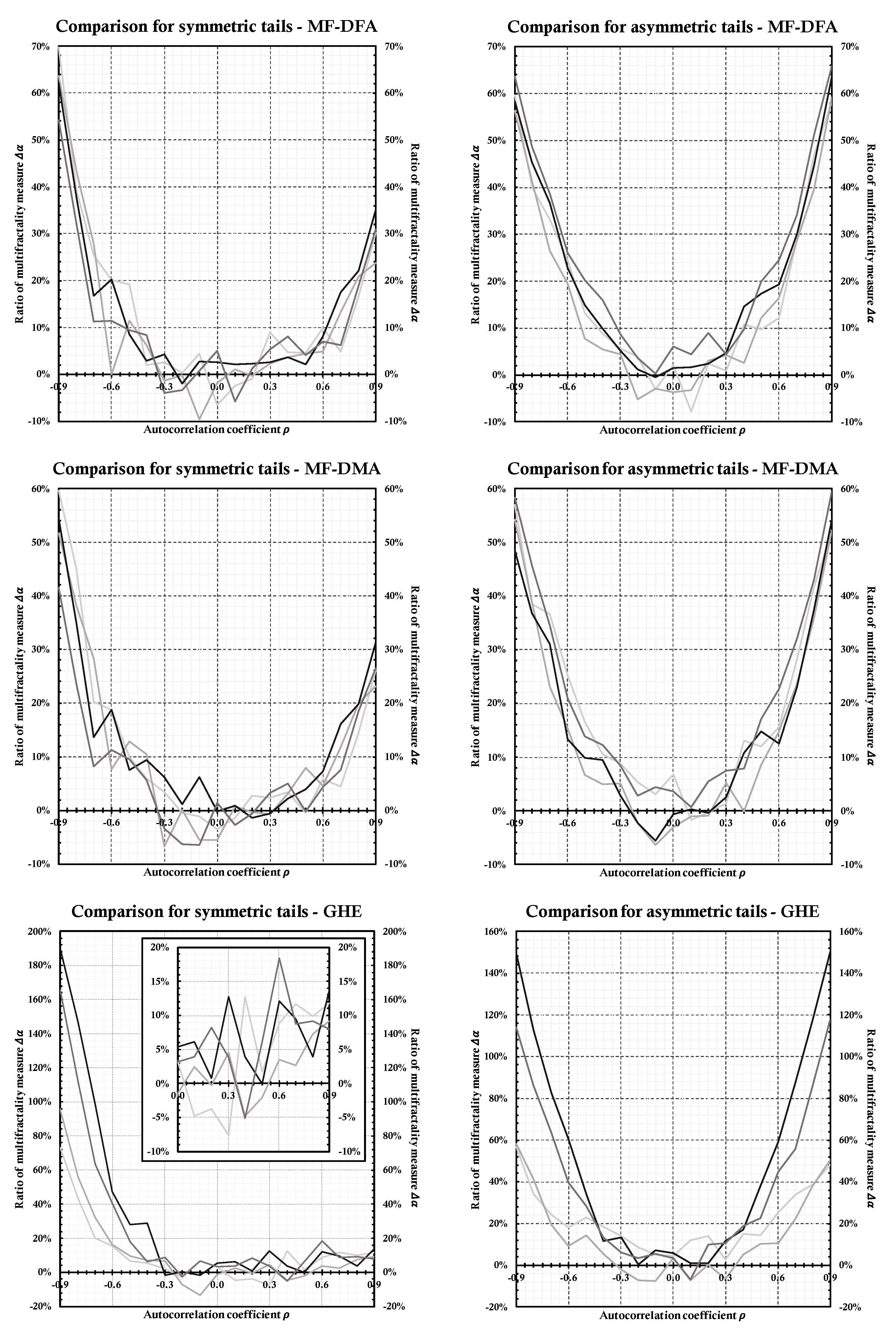
The symmetric tail auto-correlation structure, expectedly, showed a rather different picture. MF-DFA and MF-DMA still kept their J-shape from the flat correlations case but the levels changed. The GHE method showed a structural change and the relationship resembles an L-shape. For the asymmetric tails, the shape became rather symmetric for all three methods. To better understand the changes for the symmetric and asymmetric cases, we present Figure 2 which shows ratios of multifractality measures between the symmetric or asymmetric tails and their parallel flat-correlations case to see how much the quantile-dependent auto-correlations influence the multifractal properties when compared to the standard autoregressive case. Note that linear correlation is simply an average correlation over all quantiles (this has been validated by auxiliary simulations as well) [45] so that, e.g., the symmetric quantile autoregression with auto-correlations of 0.9 at the upper and the lower quartile and no serial correlation for the bulk quartiles has a linear auto-correlation coefficient of 0.45, and in parallel, the asymmetric quantile autoregression with auto-correlations of −0.9 and 0.9 at their extremes and zeros at the bulk has a linear auto-correlation coefficient of zero. Again, we find several common patterns but also some clear distinctions between the methods.
For MF-DFA and MF-DMA, the ratios collapse together with respect to the time series lengths of the underlying processes, but for GHE, the ratios are higher for the longer time series. Note that the distinction between ratios with respect to the time series length is beneficial, as longer time series make successful separation between the effects more likely. In general, the results are qualitatively very similar for MF-DFA and MF-DMA. For the case of symmetrically tailed auto-correlations, we see that it is very difficult to distinguish between the flat and tail-dependent auto-correlation structure of the series for coefficients between −0.3 and 0.3. For larger coefficients, the ratios become more prominent. For the highest levels of auto-correlations, the ratios climb up to around 30% and 60–70% for the positive and negative correlations, respectively, for both methods. However, even for auto-correlations of around ± 0.6 , the ratio does not exceed 10%. The methods are thus able to separate the effect of quantile-dependent auto-correlation structure from parallel global auto-correlation structure only for rather extreme levels of such quantile-dependent auto-correlations. Evidently, both methods perform better for negative auto-correlations. The results are somewhat better for the case of asymmetric tail correlations, reaching ratios of around 70% for the extreme auto-correlations and ratios around 20% for tail auto-correlations at ± 0.6 .
The results are quite different for GHE. In addition to being able to better separate the tail-correlations from the mean correlations with an increasing number of observations, the ratios of the singularity spectrum widths behave very differently compared to the other two methods. For the symmetric tail effects, we observe that GHE is hardly able to tell the different between the tail and the mean correlations for the positive coefficients. However, for the negative coefficients, the separation becomes clear, even though it becomes very apparent mostly for the extreme cases again. For the most extreme cases and the longest studied time series, the ratio reaches 200%. For the positive correlations, the ratio does not exceed 20% even for the most extreme cases. For the asymmetrical auto-correlations, the ratios again become symmetrical around the auto-correlation coefficient and the method clearly surpasses the other two with ratios, reaching around 150% for the highest auto-correlations and the longest time series.

5. Discussion and Conclusions

We have found a clear connection between multifractality and tail-dependent auto-correlation structures, even though it is not completely straightforward. With respect to the actual separation between the tail-specific auto-correlation structures from the standard autoregressive dynamics of the underlying series, the performance of the utilized methods varies markedly.
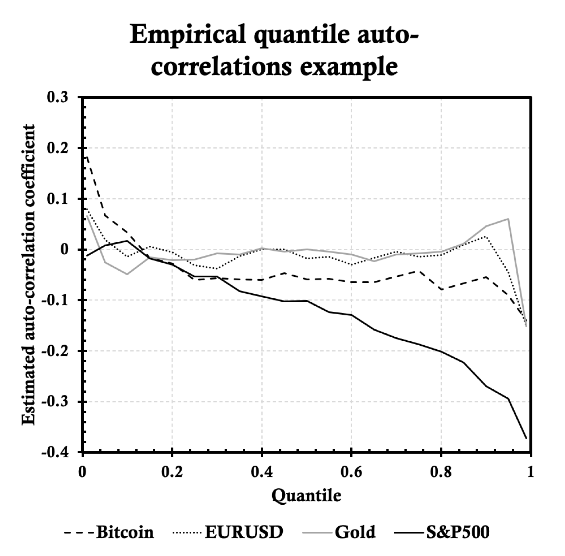
MF-DFA and MF-DMA provide satisfying results only for strong auto-correlations and GHE only for the negative ones. The results improve distinctively for the case of asymmetric tail dependencies, as not only are the levels of the ratios higher, but they are also almost perfectly symmetric. To show how this connects to actual empirical financial series, we present Figure 3 which shows that in fact the asymmetric structure of quantile auto-correlations is the more representative one. In the chart, we show the auto-correlation profiles for the logarithmic returns for the S&P 500 index, gold, EURUSD exchange rate, and Bitcoin between 1 Jan 2015 and 31 July 2020, and we observe the profiles are in fact asymmetric. Nevertheless, the levels of the coefficients are rather low and even for the most extreme asymmetry (the S&P 500 stock index), the range of the minimal and maximal auto-correlation is around 0.4. Therefore, GHE qualifies as the best method for the financial series, as it best distinguishes between the flat and quantile-dependent auto-correlation structures for the asymmetric case, although its supremacy is most apparent for longer series of 5000 observations and higher. The other two methods are thus more suitable for time series with possibly symmetric but still quantile-dependent auto-correlation structures.
In addition, we have shown that all three methods are sensitive to the standard autoregressive dynamics leading to spurious signs of multifractality. Therefore, when separating between the correlations-induced and distribution-induced multifractality, the linear auto-correlations must be carefully controlled for, i.e., plain shuffling or bootstrapping without reconstructing the linear serial correlations’ structure is not enough for clear separation between the effects. This is generally in hand with the other simulation-based studies reviewed in Jiang et al. [10], but we also found evidence and an explanation for the paradox of increased multifractality after shuffling of the original series, as first reported by Barunik et al. [44]. The latter certainly presents a challenge for theoretical justification of such behavior and/or distinguishing between the possible causes, as this might be due to the effect of the auto-correlation structure itself or the bias or inconsistency of estimators—even though a hint by Ludescher et al. [42] points to a more detailed fine-tuning of the scaling range of the estimators, which thus leads to the latter case we mention. Either way, a more detailed treatment is certainly needed.
Overall, the results of our Monte Carlo study suggest a clear connection between a non-linear correlation structure of the process and its multifractal properties. Even though the separation between the standard auto-correlations and the quantile-dependent ones is not as clear-cut as one would hope, the interaction is evident. We see that the higher the discrepancy between the bulk correlations and the tail correlations is, the higher the level of multifractality found by the utilized methods. In short, the quantile-dependent auto-correlation structures qualify as sources of multifractality and they are worth further theoretical examination.

Author Contributions

K.A. and L.K. contributed equally to this work. All authors have read and agreed to the published version of the manuscript.

Funding

The research leading to these results has received funding from the Czech Science Foundation under project number 17-12386Y and the PRIMUS program of Charles University under project number PRIMUS/19/HUM/17.

Conflicts of Interest

The authors declare no conflict of interest.

References

  1. Novikov, E.A. Intermittency and scale similarity in the structure of a turbulent flow. J. Appl. Math. Mech. 1971, 35, 231–241. [Google Scholar] [CrossRef]
  2. Mandelbrot, B.B. Possible refinement of the lognormal hypothesis concerning the distribution of energy dissipation in intermittent turbulence. Stat. Model. Turbul. Lect. Notes Phys. 1972, 12, 333–351. [Google Scholar]
  3. Mandelbrot, B.B. Intermittent turbulence in self-similar cascades: Divergence of high moments and dimension of the carrier. J. Fluid Mech. 1974, 62, 331–358. [Google Scholar] [CrossRef]
  4. Grassberger, P. Generalized dimensions of strange attractors. Phys. Lett. 1983, 97, 27–230. [Google Scholar] [CrossRef]
  5. Grassberger, P. Generalizations of the Hausdorff dimension of fractal measures. Phys. Lett. 1985, 107, 101–105. [Google Scholar] [CrossRef]
  6. Hentschel, H.G.E.; Procaccia, I. The infinite number of generalized dimensions of fractals and strange attractors. Phys. D 1983, 8, 435–444. [Google Scholar] [CrossRef]
  7. Müller, U.A.; Dacorogna, M.; Olsen, R.B.; Pictet, O.V.; Schwarz, M.; Morgenegg, C. Statistical study of foreign exchange rates, empirical evidence of a price change scaling law, and intraday analysis. J. Bank. Financ. 1990, 14, 1189–1208. [Google Scholar] [CrossRef]
  8. Ghashghaie, S.; Breymann, W.; Peinke, J.; Talkner, P.; Dodge, Y. Turbulent cascades in foreign exchange markets. Nature 1996, 381, 767–770. [Google Scholar] [CrossRef]
  9. Mandelbrot, B.B. A multifractal walk down Wall Street. Sci. Am. 1999, 280, 70–73. [Google Scholar] [CrossRef]
  10. Jiang, Z.-Q.; Xie, W.-J.; Zhou, W.-X.; Sornette, D. Multifractal analysis of financial markets: A review. Rep. Prog. Phys. 2019, 82, 125901. [Google Scholar] [CrossRef] [PubMed] [Green Version]
  11. Cont, R. Empirical properties of asset returns: Stylized facts and statistical issues. Quant. Financ. 2001, 1, 223–236. [Google Scholar] [CrossRef]
  12. Chakraborti, A.; Toke, I.M.; Patriarca, M.; Abergel, F. Econophysics review: I. Empirical facts. Quant. Financ. 2011, 11, 991–1012. [Google Scholar] [CrossRef] [Green Version]
  13. Chakraborti, A.; Toke, I.M.; Patriarca, M.; Abergel, F. Econophysics review: II. Agent-based models. Quant. Financ. 2011, 11, 1013–1041. [Google Scholar] [CrossRef] [Green Version]
  14. Kantelhradt, J.W.; Zschiegner, S.A.; Koscielny-Bunde, E.; Havlin, S.; Bunde, A.; Stanley, H.E. Multifractal detrended fluctuation analysis of nonstationary time series. Phys. A 2002, 316, 87–114. [Google Scholar] [CrossRef] [Green Version]
  15. Matteo, T.D.; Aste, T.; Dacorogna, M.M. Long-term memories of developed and emerging markets: Using the scaling analysis to characterize their stage of development. J. Bank. Financ. 2005, 29, 827–851. [Google Scholar] [CrossRef] [Green Version]
  16. Matteo, T.D. Multi-scaling in finance. Quant. Financ. 2007, 7, 21–36. [Google Scholar] [CrossRef]
  17. Bollerslev, T. Generalized autoregressive conditional heteroskedasticity. J. Econom. 1986, 31, 307–327. [Google Scholar] [CrossRef] [Green Version]
  18. Bollerslev, T. Modelling the coherence in short-run nominal exchange rates: A multivariate generalized arch model. Rev. Econ. Stat. 1990, 72, 498–505. [Google Scholar] [CrossRef]
  19. Muzy, J.-F.; Sornette, D.; Delour, J.; Arneodo, A. Multifractal returns and hierarchical portfolio theory. Quant. Financ. 2001, 1, 131–148. [Google Scholar] [CrossRef]
  20. Mandelbrot, B.B.; Fisher, A.J.; Calver, L.E. A multifractal model of asset returns. Cowles Found. Discuss. Pap. 1997, 1164, 1–31. [Google Scholar]
  21. Mandelbrot, B.B. Scaling in financial prices: III. Cartoon Brownian motions in multifractal time. Quant. Financ. 2001, 1, 427–440. [Google Scholar] [CrossRef]
  22. Calvet, L.E.; Fisher, A.J. Forecasting multifractal volatility. J. Econom. 2001, 105, 27–58. [Google Scholar] [CrossRef] [Green Version]
  23. Calvet, L.E.; Fisher, A.J. How to forecast long-run volatility: Regime switching and the estimation of multifractal processes. J. Financ. Econom. 2004, 2, 49–83. [Google Scholar] [CrossRef]
  24. Bacry, E.; Delour, J.; Muzy, J.F. Multifractal random walk. Phys. Rev. E 2001, 64, 026103. [Google Scholar] [CrossRef] [PubMed] [Green Version]
  25. Calvet, L.E.; Fisher, A.J. Multifractal Volatility: Theory, Forecasting, and Pricing; Academic Press: Burlington, MA, USA, 2008. [Google Scholar]
  26. Kukacka, J.; Kristoufek, L. Do ‘complex’ financial models really lead to complex dynamics? agent-based models and multifractality. J. Econ. Dyn. Control 2020, 113, 103855. [Google Scholar] [CrossRef]
  27. Kukacka, J.; Kristoufek, L. Does Calibration Affect the Complexity of Agent-Based Models? A Multifractal Grid Analysis. Technical Report, SSRN. 2020. Available online: https://ssrn.com/abstract=3654362 (accessed on 13 October 2020).
  28. Beran, J. Statistics for Long-Memory Processes. In Monographs on Statistics and Applied Probability; Chapman and Hall: New York, NY, USA, 1994. [Google Scholar]
  29. Calvet, L.E.; Fisher, A.J. Multifractality in asset returns: Theory and evidence. Rev. Econ. Stat. 2002, 84, 381–406. [Google Scholar] [CrossRef]
  30. Samorodnitsky, G. Long range dependence. Found. Trends Stoch. Syst. 2006, 1, 163–257. [Google Scholar] [CrossRef]
  31. Kantelhardt, J.W. Encyclopedia of Complexity and Systems Science; Chapter Fractal and multifractal time series; Springer-Veral: New York, NY, USA, 2009; pp. 3754–3779. [Google Scholar]
  32. Peng, C.; Buldyrev, S.; Goldberger, A.; Havlin, S.; Simons, M.; Stanley, H. Finite-size effects on long-range correlations: Implications for analyzing DNA sequences. Phys. Rev. E 1993, 47, 3730–3733. [Google Scholar] [CrossRef]
  33. Alessio, E.; Carbone, A.; Castelli, G.; Frappietro, V. Second-order moving average and scaling of stochastic time series. Eur. Phys. J. B 2002, 27, 197–200. [Google Scholar] [CrossRef]
  34. Vandewalle, N.; Ausloos, M. Crossing of two mobile averages: A method for measuring the roughness exponent. Phys. Rev. E 1998, 58, 6832–6834. [Google Scholar] [CrossRef]
  35. Matteo, T.D.; Aste, T.; Dacorogna, M. Scaling behaviors in differently developed markets. Phys. A 2003, 324, 183–188. [Google Scholar] [CrossRef]
  36. Peng, C.; Buldyrev, S.; Havlin, S.; Simons, M.; Stanley, H.; Goldberger, A. Mosaic organization of DNA nucleotides. Phys. Rev. E 1994, 49, 1685–1689. [Google Scholar] [CrossRef] [Green Version]
  37. Roger, K.; Zhijie, X. Quantile autoregression. J. Am. Stat. Assoc. 2006, 101, 980–990. [Google Scholar]
  38. Sklar, A. Fonctions de répartition à n dimensions et leurs marges. Publications de l’Institut de Statistique de l’Université de Paris 1959, 8, 229–231. [Google Scholar]
  39. Eric, B.; Mark, S. Dynamic copula quantile regressions and tail area dynamic dependence in forex markets. Eur. J. Financ. 2009, 15, 721–750. [Google Scholar]
  40. Xiaohong, C.; Roger, K.; Zhijie, X. Copula-based nonlinear quantile autoregression. Econom. J. 2009, 12, S50–S67. [Google Scholar]
  41. Rak, R.; Grech, D. Quantitative approach to multifractality induced by correlations and broad distribution of data. Phys. A 2018, 508, 48–66. [Google Scholar] [CrossRef] [Green Version]
  42. Ludescher, J.; Kantelhardt, B.M.I.J.W.; Schumann, A.Y.; Bunde, A. On spurious and corrupted multifractality: The effects of additive noise, short-term memory and periodic trends. Phys. A 2011, 390, 2480–2490. [Google Scholar] [CrossRef]
  43. Pamula, G.; Grech, D. Influence of the maximal fluctuation moment order q on multifractal records normalized by finite-size effects. Europhys. Lett. 2014, 105, 50004. [Google Scholar] [CrossRef]
  44. Barunik, J.; Aste, T.; Matteo, T.D.; Liu, R. Understanding the source of multifractality in financial markets. Phys. A 2012, 391, 4234–4251. [Google Scholar] [CrossRef] [Green Version]
  45. Greenwood-Nimmo, M.J.; Huang, J.; Shin, Y. Risk and return spillovers among the g10 currencies. J. Financ. Mark. 2016, 31, 43–62. [Google Scholar] [CrossRef]
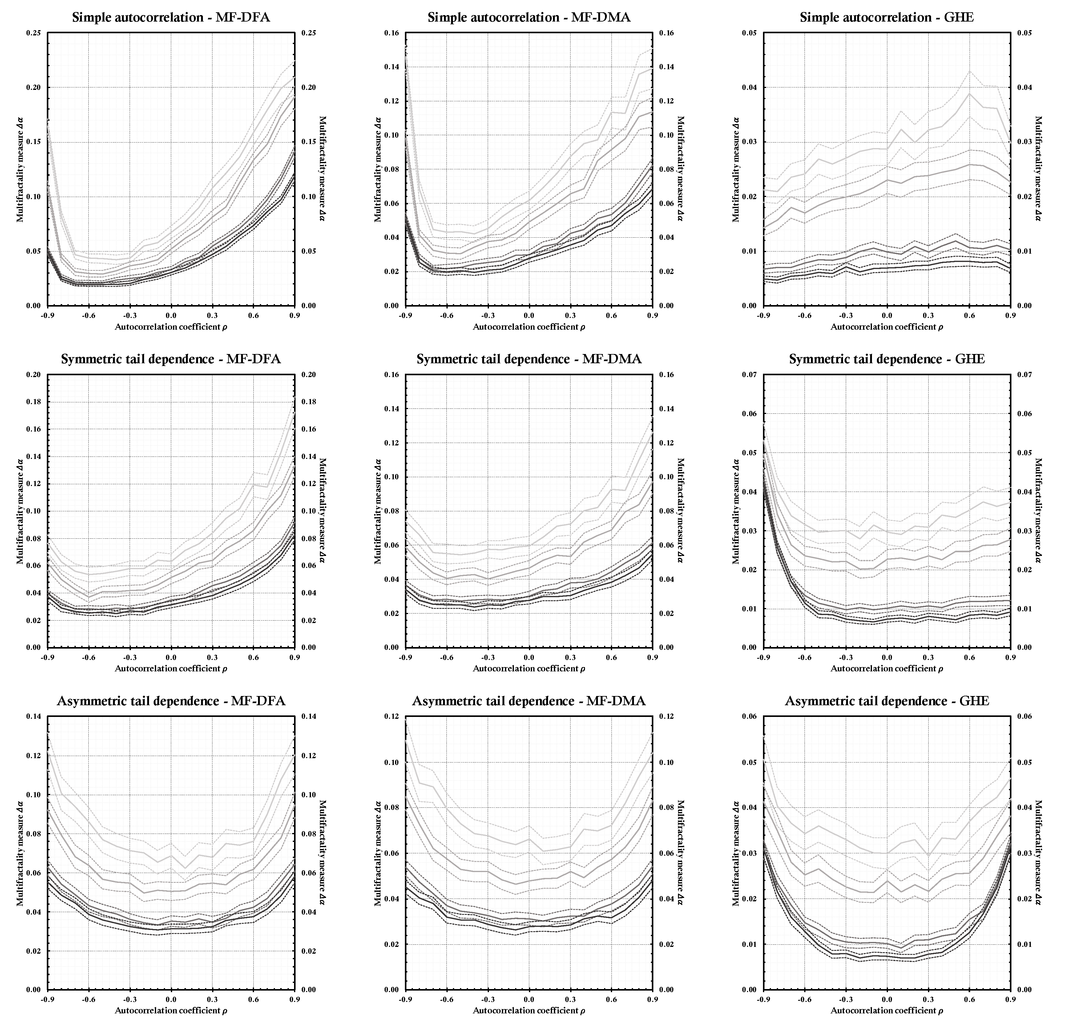
Figure 1. Multifractal range Δ α . Multifractal ranges are shown for processes with Gaussian copulas with (top) constant correlation coefficients, (middle) symmetric tail dependence, and (bottom) and asymmetric tail dependence for MF-DFA (left), MF-DMA (center), and GHE (right). The solid lines represent the mean values of the 1000 simulations for the given settings and the dashed lines represent the 95% confidence bands as the respective quantiles of the simulated distribution. The lighter the color, the longer the generated time series (black for T = 500 and light gray for T = 10,000.
Mathematics 08 01767 g001
Figure 2. Multifractal range comparison. The ratios between the singularity spectrum widths for the (a)symmetric quantile-dependent auto-correlation processes and their respective linear autoregressive counterparts are shown. The solid lines represent the ratios, and the lighter the color, the longer the generated time series.
Mathematics 08 01767 g002
Figure 3. Empirical example of the quantile auto-correlation structure. Estimated quantile-dependent auto-correlation coefficients are reported for Bitcoin, EURUSD exchange rate, gold, and S&P 500 for the period between 1 Jan 2015 and 31 July 2020. Datasets have been obtained from finance.yahoo.com.
Mathematics 08 01767 g003