The Combined Estimator for Stochastic Equations on Graphs with Fractional Noise

Abstract

In the present paper, we study the problem of estimating a drift parameter in stochastic evolution equations on graphs. We focus on equations driven by fractional Brownian motions, which are particularly useful e.g., in biology or neuroscience. We derive a novel estimator (the combined estimator) and prove its strong consistency in the long-span asymptotic regime with a discrete-time sampling scheme. The promising performance of the combined estimator for finite samples is examined under various scenarios by Monte Carlo simulations.

1. Introduction

Evolution equations on graphs and networks have proven to be a useful tool for modeling dynamics of various phenomena in many diverse fields, such as biology, engineering, statistical physics, social sciences, economics etc., for several applications of such models (such as sensor networks, nanosystems, multiagent coordination, social networks etc.); see e.g., [1] and references therein. Many real-world phenomena are affected by random effects (random forcing). These effects can be included in an evolution equation as a stochastic noise term. Evolution equations on graphs with stochastic noise have been studied e.g., in [1]. A direct application in neurobiology motivated the study of a specific type of dynamical models on graphs with fractional noise (the noise generated by a fractional Brownian motion) presented in [2]. Fractional Brownian motion has become a popular tool to model random noise with memory (with auto-correlation), which is desirable in many diverse fields (see e.g., monographs [3,4] for discussion).

Another motivation for studying stochastic evolution equations on graphs comes from the discretization of parabolic stochastic partial differential equations (SPDEs) in space domain, where the selected spatial discretization method determines the evolution operator in the equation (cf. [5]).

In this paper, we consider the problem of estimating an unknown drift parameter in stochastic evolution equations (sEE) on graphs with fractional noise. Estimating a drift parameter in various stochastic differential equations has been considered by many authors. A great amount of literature has been devoted to equations with white noise (generated by a standard Brownian motion with uncorrelated increments), where the maximum-likelihood approach dominates; see for example the classical monograph [6] for 1-dimensional equations or the recent overview paper [7] for equations in ∞-dimensional spaces, to name just a few. Specific problems arise in equations with fractional noise (generated by a fractional Brownian motion with autocorrelated increments); see e.g., books [8,9] for discussion of various approaches to parameter estimation in this setting. We are not aware of any study on parameter estimation in the context of sEE on graphs with fractional noise, although it may be of a great interest for both researchers and practitioners, as it corresponds to inferring certain properties of a random dynamical system on a graph based on observing its evolution in time. This paper is supposed to bridge this gap.

Our paper is organized as follows. In Section 2, we specify the basic setting of the estimation problem. In Section 3, we recall the definition of a fractional Brownian motion, its basic properties and calculus. Moreover, we provide a short overview of the concepts of mild solutions to stochastic evolution equations in both physical and frequency domain. Section 4 is devoted to the introduction, calculation and strong consistency of the combined estimator—the main contribution of this paper. Illustration of the actual performance of the combined estimator in several scenarios is presented in Section 5 with Monte Carlo simulations. Main findings and results of this paper are summarized in Section 6.

2. Problem Setup

Consider an undirected, connected, finite graph $G=(V,E)$ with a set of vertices $V=\{v_1,\cdots ,v_N\}$ and a set of edges E. Denote by ${\mathbb{R}}^V$ a finite-dimensional Hilbert space of the real-valued functions on V with the canonical scalar product defined by $\langle x,y\rangle ={\sum }_{v\in V}x\left(v\right)y\left(v\right)$. Note that the indicator functions $e_v=1_v$ for $v\in V$ form the canonical orthonormal basis of ${\mathbb{R}}^V$. Recall that the combinatorial graph Laplacian L on a graph G is a self-adjoint, positive semidefinite, linear operator on ${\mathbb{R}}^V$, characterized by the following matrix:

$$L={\left[l_{v,w}\right]}_{v,w\in V};l_{v,w}=\left\{\begin{array}{cc}\mathrm{deg}\left(v\right)\hfill & \mathrm{if}v=w\hfill \\ -1\hfill & \mathrm{if}\{v,w\}\in E\hfill \\ 0\hfill & \mathrm{else},\hfill \end{array}\right.\forall v,w\in V,$$

(1)

where $\mathrm{deg}\left(v\right)$ is number of edges connected to v (the degree of v).

As a motivation (and a toy model) for further studies, consider a simple heat equation on the graph G with stochastic forcing,

$$\begin{array}{cc}\hfill & \frac{\partial x}{\partial t}(t,v)=-\lambda \left(Lx\left(t\right)\right)\left(v\right)+\eta (t,v),\mathrm{for}t\in {\mathbb{R}}_{+}\mathrm{and}v\in V,\hfill \end{array}$$

(2)

$$\begin{array}{cc}\hfill & x(0,.)\in {\mathbb{R}}^V,\hfill \end{array}$$

(3)

where $x(t,v)$ is a real-valued state variable at vertex v and time t, $\lambda \in {\mathbb{R}}_{+}$ is an unknown parameter (heat conductivity), L is the combinatorial graph Laplacian and $\eta (t,v)$ represents a noise (stochastic) term, being a formal time-derivative of a (fractional) Brownian motion.

Since the classical (strong) derivative of a (fractional) Brownian motion does not exist, we reformulate the above stochastic heat equation rigorously as a sEE on the finite-dimensional Hilbert space ${\mathbb{R}}^V$:

$$\begin{array}{cc}\hfill d{X}_t& =-\lambda L{X}_{t}dt+\mathsf{\Phi }d{B}_t^H,\hfill \\ \hfill X_0& =x(0,.)\in {\mathbb{R}}^V,\hfill \end{array}$$

(4)

where ${\left\{X_t\right\}}_{t\ge 0}={\left\{x(t,.)\right\}}_{t\ge 0}$ is an ${\mathbb{R}}^V$-valued random process, $\lambda \in {\mathbb{R}}_{+}$ is an unknown drift parameter and L is the combinatorial graph Laplacian. For the noise (stochastic) part, $B^H$ denotes the cylindrical fractional Brownian motion on ${\mathbb{R}}^V$ with Hurst index H and $\mathsf{\Phi }$, being a bounded operator on ${\mathbb{R}}^V$, determines the correlations between vertices.

Motivated by the above example, we consider the parameter estimation problem in an evolution equation on ${\mathbb{R}}^V$ of the following form in this paper:

$$\begin{array}{cc}\hfill d{X}_t& =-A\left(\lambda \right)X_{t}dt+\mathsf{\Phi }d{B}_t^H,\hfill \\ \hfill X_0& =x(0,.)\in {\mathbb{R}}^V,\hfill \end{array}$$

(5)

where the drift operator $A\left(\lambda \right)$ is a linear, self-adjoint, positive semidefinite operator (matrix) on ${\mathbb{R}}^V$. It depends on an unknown (potentially d-dimensional) parameter $\lambda \in C\subset {\mathbb{R}}^d$, with C being compact. In the context of graph theory, the operator A may represent (weighted) graph Laplacian, in-degree Laplacian (for oriented graphs), d-path Laplacian (for non-local interactions, see [10]) or other linear operators. $B^H$ is again the cylindrical fractional Brownian motion on ${\mathbb{R}}^V$ with Hurst index $H\ge 1/2$ (the regular case with positively auto-correlated increments) and $\mathsf{\Phi }$ a bounded linear operator on ${\mathbb{R}}^V$.

We address the problem of estimating the unknown drift parameter $\lambda$ based on a single trajectory of a solution to evolution Equation (5) observed at discrete time instants with a time step $h>0$, i.e., based on ${\left\{X_{ih}\right\}}_{i=0,\cdots n}$. We assume that the time step $h>0$ is fixed and the time horizon goes to infinity, $T=nh\to \infty$, i.e., the discrete sampling scheme with long-span asymptotics. Literature on drift estimation for multidimensional sEE with the discrete sampling scheme and long-span asymptotics is rather sparse. In this respect, let us mention papers [11,12,13] considering SPDEs with white-in-time noise, and paper [14] focused on infinite-dimensional sEE with fractional noise. The so-called minimum-contrast estimator (MCE) studied in the latter paper is plausible in our setting, if the projection of a solution to the eigenspaces corresponding to strictly positive eigenvalues is considered (to ensure ergodicity). However, the comparison in the recent paper [15] shows that the ergodic estimator (the counterpart to the MCE in one-dimensional setting) provides less accurate estimates compared to the conditional least-squares estimator (introduced in [15]), which turned out to be a very powerful estimator of the unknown drift in models with autocorrelated noise. Hence, we generalize the idea of the conditional least-squares approach into the multi-dimensional framework. To enhance the efficiency of the estimator, we combine the conditional least-squares approach in the time domain (where the covariance structure is complicated) with a maximum-likelihood approach in the space domain (with rather simple covariance structure), which leads to a novel estimator—the combined estimator (CoE).

The value of the Hurst index H is considered to be known. If this is not the case, it can be estimated in advance (before an evaluation of the combined estimator) by some of many available methods—see for example [16,17,18] to name just a few. The estimated H can subsequently be used in the CoE of the drift parameter similarly to the approach applied in [19]. The simultaneous estimation of $\lambda$ and H in sEE on graphs is outside the scope of this work and could be a potential direction for further research.

3. Preliminaries

3.1. Fractional Brownian Motion and Its Calculus

In this subsection, we briefly introduce the fractional Brownian motion (fBm) and specifics of the stochastic calculus w.r.t. the fBm. For further reading, we refer the interested reader to the monographs [3,4] and references therein.

The one-dimensional fractional Brownian motion ${\left\{{\beta }^H\left(t\right)\right\}}_{t\ge 0}$ is a centered continuous real-valued Gaussian process starting from zero and having the following covariance structure

$$\begin{array}{c}\hfill \mathrm{E}\left({\beta }^H\left(s\right){\beta }^H\left(t\right)\right)=\frac{1}{2}\left(s^{2H}+t^{2H}-{|s-t|}^{2H}\right),s,t\ge 0.\end{array}$$

The covariance depends on a parameter $H\in (0,1)$, which is called the Hurst index. If $H=1/2$, fBm has independent increments and it coincides with a standard Brownian motion (the Wiener process). If $H>1/2$, fBm has positively correlated increments and it exhibits a long-range dependence. It enjoys increasing popularity in many applications where long-range dependence is observed. It also has more regular trajectories than the Wiener process (in terms of the Hölder continuity). The case $H<1/2$ (not considered in this work) leads to negatively correlated increments, less regular trajectories and serious difficulties when integrating w.r.t. the fBm. A two-sided fBm is again a centered continuous Gaussian process ${\left\{{\beta }^H\left(t\right)\right\}}_{t\in \mathbb{R}}$ with t ranging over the whole $\mathbb{R}$, ${\beta }^H\left(0\right)=0$ and

$$\begin{array}{c}\hfill \mathrm{E}\left({\beta }^H\left(s\right){\beta }^H\left(t\right)\right)=\frac{1}{2}\left({\left|s\right|}^{2H}+{\left|t\right|}^{2H}-{|s-t|}^{2H}\right),s,t\in \mathbb{R}.\end{array}$$

The N-dimensional fBm ${\left\{B^H\left(t\right)\right\}}_{t\ge 0}={\left\{{({\beta }_1^H\left(t\right),\dots ,{\beta }_N^H\left(t\right))}^T\right\}}_{t\ge 0}$ is an N-dimensional random process whose coordinates are mutually independent real-valued fBm with the same Hurst index H.

Consider a fBm ${\left\{{\beta }^H\left(t\right)\right\}}_{t\ge 0}$ with $H>1/2$ and a deterministic step function $\psi \left(s\right)={\displaystyle \sum _{k=1}^M}{c}_k{I}_{[t_k,t_{k+1}]}\left(s\right)$. The Wiener integral of $\psi$ w.r.t. ${\beta }^H$ is defined by formula

$$\begin{array}{c}\hfill {\int }_0^{\infty }\psi \left(s\right)d{\beta }^H\left(s\right)=\sum _{k=1}^M{c}_k\left({\beta }^H\left(t_{k+1}\right)-{\beta }^H\left(t_k\right)\right).\end{array}$$

As a consequence, we obtain the following isometry for any pair of deterministic step functions $\psi$ and $\varphi$:

$$\begin{array}{c}\hfill \mathrm{E}\left({\int }_0^{\infty }\psi \left(t\right)d{\beta }^H\left(t\right){\int }_0^{\infty }\varphi \left(s\right)d{\beta }^H\left(s\right)\right)={\int }_0^{\infty }{\int }_0^{\infty }\psi \left(t\right)\varphi \left(s\right)H(2H-1){|t-s|}^{2H-2}\mathrm{d}t\mathrm{d}s=\langle \psi ,\varphi \rangle .\end{array}$$

(6)

This isometry enables us to extend the definition of the Wiener integral w.r.t. a fBm to all elements of the completion of the space of deterministic step functions w.r.t. the scalar product $\langle .,.\rangle$ defined above. In result, Formula (6) holds true for all functions from this completion, see also [20]. This formula is extremely useful for the construction of the combined estimator below.

3.2. Solution to sEE in Physical and Frequency Domain

For the reader’s convenience, we recall the concept of mild solution to (5) in physical domain. It reads:

$$X_t=e^{-A\left(\lambda \right)t}{X}_0+{\int }_0^t{e}^{-A\left(\lambda \right)(t-s)}\mathsf{\Phi }d{B}_s^H,\mathrm{where}{e}^{-A\left(\lambda \right)t}=\sum _{j=0}^{\infty }\frac{{[-A\left(\lambda \right)]}^j{t}^j}{j!}.$$

(7)

The existence of the mild solution was established (in more general setting of sEE on Hilbert spaces) in papers [21] for $H>1/2$ and [22] for $H<1/2$, or in paper [23].

When studying the solution, we can switch from the physical to the frequency domain. It provides us with an easy-to-handle formula of the solution, which will be useful both for the simulation and parameter estimation in the sequel. Start with the spectral decomposition of the self-adjoint, positive semidefinite matrix $A\left(\lambda \right)$:

$$A\left(\lambda \right)=G\left(\lambda \right)D\left(\lambda \right)G{\left(\lambda \right)}^T,$$

(8)

where $G\left(\lambda \right)$ is a $N\times N$ matrix whose columns are orthonormal eigenvectors ${\left\{g_k\left(\lambda \right)\right\}}_{k=1\cdots N}$ of $A\left(\lambda \right)$ and $D\left(\lambda \right)=diag\{{\alpha }_1\left(\lambda \right),\cdots ,{\alpha }_N\left(\lambda \right)\}$ is a diagonal matrix formed by the corresponding non-negative eigenvalues. It easily follows:

$$e^{-A\left(\lambda \right)t}=G\left(\lambda \right){\mathcal{E}}_t\left(\lambda \right)G{\left(\lambda \right)}^T,\mathrm{where}{\mathcal{E}}_t\left(\lambda \right)=diag\{e^{-{\alpha }_1\left(\lambda \right)t},\cdots ,e^{-{\alpha }_N\left(\lambda \right)t}\}.$$

(9)

With this decomposition at hand, we can consider the solution to (5) in frequency domain:

$$F_t=G{\left(\lambda \right)}^T{X}_t,$$

(10)

which is given by the mild formula

$$F_t={\mathcal{E}}_t\left(\lambda \right)F_0+{\int }_0^t{\mathcal{E}}_{t-s}\left(\lambda \right)d{\tilde{B}}_s^H,$$

(11)

where

$${\tilde{B}}_t^H=G{\left(\lambda \right)}^T\mathsf{\Phi }{B}_t^H,t\ge 0.$$

(12)

Since this system is diagonal, we can write explicit formulas for individual entries of $F_t$. Denote

$$F_t={(f_1\left(t\right),\cdots ,f_N\left(t\right))}^T\mathrm{and}{\tilde{B}}_t^H={({\tilde{\beta }}_1^H\left(t\right),\cdots ,{\tilde{\beta }}_N^H\left(t\right))}^T.$$

Then ${\left\{f_k\left(t\right)\right\}}_{t\ge 0}$ are real-valued fractional Ornstein-Uhlenbeck processes, as seen from the formulas

$$f_k\left(t\right)=e^{-{\alpha }_k\left(\lambda \right)t}{f}_k\left(0\right)+{\int }_0^t{e}^{-{\alpha }_k\left(\lambda \right)(t-s)}d{\tilde{\beta }}_k^H\left(s\right),k=1,\cdots ,N.$$

(13)

To eliminate the stochastic Wiener integral from the expression above, we can apply the integration by parts formula to get

$$f_k\left(t\right)=e^{-{\alpha }_k\left(\lambda \right)t}{f}_k\left(0\right)+{\tilde{\beta }}_k^H\left(t\right)-{\int }_0^t{\tilde{\beta }}_k^H\left(s\right)e^{-{\alpha }_k\left(\lambda \right)(t-s)}{\alpha }_k\left(\lambda \right)ds,k=1,\cdots ,N.$$

(14)

The solution formula above is particularly useful for simulations, because it contains only Riemann integral and no stochastic integration is needed.

4. Combined Estimator

To estimate the unknown parameter $\lambda$ in (5), we observe a single realization of the process ${\left\{X_{ih}\right\}}_{i=0,\cdots n}$. It is an $(N\times (n+1\left)\right)$-dimensional Gaussian vector, so a natural choice would be to take the maximum-likelihood estimator. However, the evaluation of such an estimator would be extremely consuming, both in terms of CPU time and memory, especially for large n. This is due to the complicated structure of the covariance matrix with respect to time domain $i=0,\cdots n$ resulting from the long-range dependence of the fractional Brownian motion with $H>1/2$. Hence, some approximation to MLE has to be considered (cf. e.g., [24]). In this section, we study an approximation based on the conditional least-squares technique. This approach has recently been introduced and studied (with promising results) in [15] for real-valued fractional Ornstein-Uhlenbeck processes.

4.1. Combined Estimator in Physical Domain

The main idea of the conditional least-squares technique is to consider the following linear model

$$X_{t+h}={\mathrm{E}}_{\lambda }\left[X_{t+h}\right|X_t]+{\eta }_t={\mu }_t(X_t,\lambda )+{\eta }_t,$$

(15)

where ${\mathrm{E}}_{\lambda }\left[X_{t+h}\right|X_t]$ means the conditional expectation of $X_{t+h}$, conditioned by $X_t$, where the process X is given by (5) with parameter value $\lambda$. Conditioning eliminates the unwanted correlations between explanatory variables and error terms in model (15), which enables the application of the least-squares technique.

To design the ultimate form of the least-squares criterion to be minimized, we have to decide about the space-norm to be applied to the vectors $X_{t+h}-{\mathrm{E}}_{\lambda }\left[X_{t+h}\right|X_t]$. In this aspect, we stick to the maximum-likelihood technique, which is well suited e.g., for the white-in-space noise ($\mathsf{\Phi }$ is diagonal). Notice the N-dimensional Gaussian conditional distribution

$${\mathrm{Law}}_{\lambda }\left(X_{t+h}\right|X_t)=\mathcal{N}\left({\mu }_t(X_t,\lambda ),{\mathsf{\Sigma }}_t\left(\lambda \right)\right),$$

(16)

and the corresponding log-likelihood function (for a fixed t):

$$l_t(X_{t+h},\lambda |X_t)=Const-\frac{1}{2}log\left(det\left[{\mathsf{\Sigma }}_t\left(\lambda \right)\right]\right)-\frac{1}{2}{\left(X_{t+h}-{\mu }_t(X_t,\lambda )\right)}^T{\left[{\mathsf{\Sigma }}_t\left(\lambda \right)\right]}^{-1}\left(X_{t+h}-{\mu }_t(X_t,\lambda )\right).$$

To express ${\mu }_t$ and ${\mathsf{\Sigma }}_t$ explicitly, recall

$$X_{t+h}=e^{-A\left(\lambda \right)h}{X}_t+{\xi }_t,$$

where

$$X_t=e^{-A\left(\lambda \right)t}{X}_0+{\int }_0^t{e}^{-A\left(\lambda \right)(t-s)}\mathsf{\Phi }d{B}^H\left(s\right),{\xi }_t={\int }_t^{t+h}{e}^{-A\left(\lambda \right)(t+h-s)}\mathsf{\Phi }d{B}^H\left(s\right).$$

Now consider the more complicated case $H>1/2$ (the simpler case $H=1/2$ is discussed in Remark 1). Utilizing isometry (6), we get the (co)variance matrices

$$\begin{array}{cc}\hfill & var\left(X_t\right)=H(2H-1){\int }_{-t}^0{\int }_{-t}^0{e}^{A\left(\lambda \right)r}\mathsf{\Phi }{\mathsf{\Phi }}^T{e}^{A\left(\lambda \right)s}{|r-s|}^{2H-2}dsdr,\hfill \end{array}$$

(17)

$$\begin{array}{cc}\hfill & var\left({\xi }_t\right)=H(2H-1){\int }_{-h}^0{\int }_{-h}^0{e}^{A\left(\lambda \right)r}\mathsf{\Phi }{\mathsf{\Phi }}^T{e}^{A\left(\lambda \right)s}{|r-s|}^{2H-2}dsdr,\hfill \end{array}$$

(18)

$$\begin{array}{cc}\hfill & cov({\xi }_t,X_t)=H(2H-1)e^{-A\left(\lambda \right)h}{\int }_0^h{\int }_{-t}^0{e}^{A\left(\lambda \right)r}\mathsf{\Phi }{\mathsf{\Phi }}^T{e}^{A\left(\lambda \right)s}{|r-s|}^{2H-2}dsdr.\hfill \end{array}$$

(19)

The joint multivariate normality of $X_t$ and ${\xi }_t$ leads to

$$\begin{array}{cc}\hfill & {\mu }_t(X_t,\lambda )={\mathrm{E}}_{\lambda }\left[X_{t+h}\right|X_t]=\left\{\begin{array}{cc}{e}^{-A\left(\lambda \right)h}{X}_t+cov({\xi }_t,X_t){[var\left(X_t\right)]}^{-1}(X_t-e^{-A\left(\lambda \right)t}{X}_0)\hfill & \mathrm{for}t>0\hfill \\ e^{-A\left(\lambda \right)h}{X}_t\hfill & \mathrm{for}t=0,\hfill \end{array}\right.\hfill \end{array}$$

(20)

$$\begin{array}{cc}\hfill & {\mathsf{\Sigma }}_t\left(\lambda \right)={var}_{\lambda }\left[X_{t+h}\right|X_t]=\left\{\begin{array}{cc}var\left({\xi }_t\right)-cov({\xi }_t,X_t){[var\left(X_t\right)]}^{-1}{[cov({\xi }_t,X_t)]}^T\hfill & \mathrm{for}t>0\hfill \\ var\left({\xi }_t\right)\hfill & \mathrm{for}t=0.\hfill \end{array}\right.\hfill \end{array}$$

(21)

The combination of the conditional least-squares approach in the time domain with the maximum-likelihood approach in the space domain results in the following combined estimator:

$$\widehat{\lambda }=\underset{\mathsf{\Lambda }\in C}{argmin}Q\left(\mathsf{\Lambda }\right),$$

(22)

where C is a compact subset of ${\mathbb{R}}^d$, $\mathsf{\Lambda }$ is an unknown representing the parameter to be estimated ($\lambda$ is its true value) and

$$Q\left(\mathsf{\Lambda }\right)=\sum _{t\in \{0,h\cdots ,(n-1\left)h\right\}}\left[log\left(det\left[{\mathsf{\Sigma }}_t\left(\mathsf{\Lambda }\right)\right]\right)+{\left(X_{t+h}-{\mu }_t(X_t,\mathsf{\Lambda })\right)}^T{\left[{\mathsf{\Sigma }}_t\left(\mathsf{\Lambda }\right)\right]}^{-1}\left(X_{t+h}-{\mu }_t(X_t,\mathsf{\Lambda })\right)\right],$$

(23)

with ${\mu }_t$ and ${\mathsf{\Sigma }}_t$ explicitly expressed in (20) and (21), respectively.

Remark 1.

If $H=1/2$, which corresponds to the white-in-time noise, the combined estimator coincides with classical MLE. Indeed, $X_t$ and ${\xi }_t$ are independent in this case, the Gaussian process ${\left\{X_{ih}\right\}}_{i=0,\cdots ,n}$ has Markov property and its joint distribution corresponds to the product of the conditional distributions (16). As a result, minimizing (22) is equivalent to minimizing log-likelihood function of the process. Moreover, we have simplified calculations

$$\begin{array}{cc}\hfill & {\mu }_t(X_t,\lambda )=e^{-A\left(\lambda \right)h}{X}_t,\hfill \\ \hfill & {\mathsf{\Sigma }}_t\left(\lambda \right)=var\left({\xi }_t\right)={\int }_{-h}^0{e}^{A\left(\lambda \right)s}\mathsf{\Phi }{\mathsf{\Phi }}^T{e}^{A\left(\lambda \right)s}ds.\hfill \end{array}$$

4.2. Combined Estimator in Diagonal Case

If the number of vertices N is large, evaluation of the criterion function in Formula (22) might be computationally demanding, mainly due to inversions of $N\times N$ matrices ${[var\left(X_t\right)]}^{-1}$ and ${\left[{\mathsf{\Sigma }}_t\left(\mathsf{\Lambda }\right)\right]}^{-1}$ for all $t\in \{h,2h\cdots ,nh\}$. This issue can be resolved by considering the whole problem in the spectral domain in the diagonal case. For this reason, we assume throughout this subsection that the noise term is white in space, i.e., $\mathsf{\Phi }$ is an identity matrix (possibly multiplied by a constant characterizing noise intensity):

Assumption 1

(WN).

$$\mathsf{\Phi }=\sigma Id,\sigma >0.$$

(24)

Recall the spectral decomposition of $A\left(\lambda \right)$ and $e^{-A\left(\lambda \right)t}$ given in (8) and (9), respectively. In addition, assume that the eigenvectors of operator $A\left(\lambda \right)$ do not depend on the parameter λ, i.e.,

Assumption 2

(EV).

$$G\left(\lambda \right)=G.$$

(25)

Such an assumption is satisfied if the unknown parameter λ affects only the eigenvalues of $A\left(\lambda \right)$, for example, if λ is a multiplicative constant (diffusivity or heat conductivity): $A\left(\lambda \right)=\lambda A$.

To simplify the exposition, sort the eigenvalues in descendent order, so that the first M eigenvalues are positive and the others are zeros:

$${\alpha }_1\left(\lambda \right)\ge {\alpha }_2\left(\lambda \right)\ge \cdots \ge {\alpha }_M\left(\lambda \right)>{\alpha }_{M+1}\left(\lambda \right)=\cdots ={\alpha }_N\left(\lambda \right)=0.$$

(26)

It follows

$$var\left(X_t\right)=H(2H-1){\sigma }^{2}G\left({\int }_{-t}^0{\int }_{-t}^0{\mathcal{E}}_{-r-s}\left(\lambda \right){|r-s|}^{2H-2}dsdr\right)G^T,$$

and after substitutions in integrals on the diagonal,

$$var\left(X_t\right)=H(2H-1){\sigma }^{2}Gdiag\left\{\frac{I\left({\alpha }_1\left(\lambda \right)t\right)}{{\alpha }_1{\left(\lambda \right)}^{2H}},\cdots ,\frac{I\left({\alpha }_M\left(\lambda \right)t\right)}{{\alpha }_M{\left(\lambda \right)}^{2H}},\frac{t^{2H}}{H(2H-1)},\cdots ,\frac{t^{2H}}{H(2H-1)}\right\}{G}^T,$$

where we denoted

$$I\left(x\right)={\int }_{-x}^0{\int }_{-x}^0{e}^{r+s}{|r-s|}^{2H-2}dsdr.$$

(27)

Note that using change-of-variable formula ($u=r+s$, $v=r-s$) and analytical integrating over v yields the following formula with simple one-dimensional integrals, which is numerically more stable and easier to implement:

$$I\left(x\right)=\frac{1}{2H-1}\left[e^{-2x}{\int }_0^x{e}^u{u}^{2H-1}du+{\int }_0^x{e}^{-u}{u}^{2H-1}du\right].$$

The other two (co)variance matrices can be treated similarly:

$$\begin{array}{cc}\hfill & var\left({\xi }_t\right)=H(2H-1){\sigma }^{2}Gdiag\left\{\frac{I\left({\alpha }_1\left(\lambda \right)h\right)}{{\alpha }_1{\left(\lambda \right)}^{2H}},\cdots ,\frac{I\left({\alpha }_M\left(\lambda \right)h\right)}{{\alpha }_M{\left(\lambda \right)}^{2H}},\frac{h^{2H}}{H(2H-1)},\cdots ,\frac{h^{2H}}{H(2H-1)}\right\}{G}^T,\hfill \\ \hfill & cov({\xi }_t,X_t)=H(2H-1){\sigma }^{2}G{\mathcal{E}}_h\left(\lambda \right)diag\left\{co{v}_1,\cdots ,co{v}_N\right\}{G}^T,\hfill \end{array}$$

where

$$co{v}_k=\left\{\begin{array}{cc}\frac{J({\alpha }_k\left(\lambda \right)h,{\alpha }_k\left(\lambda \right)t)}{{\alpha }_k{\left(\lambda \right)}^{2H}},\hfill & k=1,\cdots ,M,\hfill \\ \\ \frac{{(t+h)}^{2H}-t^{2H}-h^{2H}}{2H(2H-1)},\hfill & k=M+1,\cdots ,N.\hfill \end{array}\right.$$

and where we define

$$J(x,y)={\int }_0^x{\int }_{-y}^0{e}^{r+s}{|r-s|}^{2H-2}dsdr,$$

(28)

After changing variables and analytical integration, we can again simplify this double integral into simple one-dimensional integrals, which are easier to approximate numerically:

$$J(x,y)=\frac{1}{2(2H-1)}\left[e^{2x}{\int }_x^{x+y}{e}^{-u}{u}^{2H-1}du-{\int }_0^y{e}^{-u}{u}^{2H-1}du+e^{-2y}{\int }_y^{x+y}{e}^u{u}^{2H-1}du-{\int }_0^x{e}^u{u}^{2H-1}du\right].$$

Ease of inversion of diagonal matrices provides us with the simplified formula

$$\begin{array}{cc}\hfill & {\mu }_t(X_t,\lambda )=e^{-A\left(\lambda \right)h}{X}_t\hfill \\ \hfill & +Gdiag\left\{m_1,\cdots ,m_N\right\}{G}^T(X_t-e^{-A\left(\lambda \right)t}{X}_0),\hfill \end{array}$$

where

$$m_k=\left\{\begin{array}{cc}m({\alpha }_k\left(\lambda \right),t)=e^{-{\alpha }_k\left(\lambda \right)h}\frac{J({\alpha }_k\left(\lambda \right)h,{\alpha }_k\left(\lambda \right)t)}{I\left({\alpha }_k\left(\lambda \right)t\right)},\hfill & k=1,\cdots ,M,\hfill \\ \\ \frac{{(t+h)}^{2H}-t^{2H}-h^{2H}}{2t^{2H}},\hfill & k=M+1,\cdots ,N.\hfill \end{array}\right.$$

(29)

If we switch from physical to frequency domain, see (10), we get

$$\begin{array}{cc}\hfill & {\mu }_t(X_t,\lambda )=G{\mathcal{E}}_h\left(\lambda \right)F_t\hfill \\ \hfill & +Gdiag\left\{m_1,\cdots ,m_N\right\}(F_t-{\mathcal{E}}_t\left(\lambda \right)F_0).\hfill \end{array}$$

Similarly

$${\mathsf{\Sigma }}_t\left(\lambda \right)=H(2H-1){\sigma }^{2}Gdiag\{s_1,\cdots ,s_N\}{G}^T,$$

where

$$s_k=\left\{\begin{array}{cc}s({\alpha }_k\left(\lambda \right),t)=\frac{I\left({\alpha }_k\left(\lambda \right)h\right)}{{\alpha }_k{\left(\lambda \right)}^{2H}}-e^{-2{\alpha }_k\left(\lambda \right)h}\frac{J^2({\alpha }_k\left(\lambda \right)h,{\alpha }_k\left(\lambda \right)t)}{I\left({\alpha }_k\left(\lambda \right)t\right)}\frac{1}{{\alpha }_k{\left(\lambda \right)}^{2H}},\hfill & k=1,\cdots ,M,\hfill \\ \\ \frac{h^{2H}}{H(2H-1)}-\frac{{[{(t+h)}^{2H}-t^{2H}-h^{2H}]}^2}{t^{2H}4H(2H-1)},\hfill & k=M+1,\cdots ,N.\hfill \end{array}\right.$$

(30)

Now we can construct the spectral version of the criterion (23). Let $\mathsf{\Lambda }$ be again an unknown representing the parameter to be estimated ($\lambda$ is its true value) and denote by $f_k\left(t\right)$ the coefficients in frequency domain, i.e.,

$${(f_1\left(t\right),\cdots ,f_N\left(t\right))}^T={(g_1^T{X}_t,\cdots ,g_N^T{X}_t)}^T=G^T{X}_t.$$

Using this notation, we can write

$$\begin{array}{cc}\hfill & Q\left(\mathsf{\Lambda }\right)=\sum _{t\in \{0,h\cdots ,(n-1\left)h\right\}}[Nlog\left(H(2H-1){\sigma }^2\right)+\sum _{k=1}^{N}log\left(s_k\right)\hfill \\ \hfill & +\frac{1}{H(2H-1){\sigma }^2}\sum _{k=1}^N\frac{1}{s_k}{\left(f_k(t+h)-e^{-{\alpha }_k\left(\mathsf{\Lambda }\right)h}{f}_k\left(t\right)-m_k[f_k\left(t\right)-e^{-{\alpha }_k\left(\mathsf{\Lambda }\right)t}{f}_k\left(0\right)]\right)}^2],\hfill \end{array}$$

(31)

with $s_k=s_k(t,\mathsf{\Lambda })$ defined in (30) and $m_k=m_k(t,\mathsf{\Lambda })$ in (29). Note that by using spectral decomposition, we eliminated the matrix inversions from the criterion formula and integrals of matrices were substituted by real-valued integrals of the form (27) and (28). Moreover, if $k=M+1,\cdots ,N$, then neither of ${\alpha }_k\left(\mathsf{\Lambda }\right)$, $s_k(\mathsf{\Lambda },t)$ and $m_k(\mathsf{\Lambda },t)$ depend on $\mathsf{\Lambda }$. As a result, minimizing $Q\left(\mathsf{\Lambda }\right)$ with respect to $\mathsf{\Lambda }$ is the same as minimizing its reduced version:

$$\begin{array}{cc}& Q_M\left(\mathsf{\Lambda }\right)=\sum _{t\in \{0,h\cdots ,(n-1\left)h\right\}}[Mlog\left(H(2H-1){\sigma }^2\right)+\sum _{k=1}^{M}log\left(s({\alpha }_k\left(\mathsf{\Lambda }\right),t)\right)\hfill \\ & +\frac{1}{H(2H-1){\sigma }^2}\sum _{k=1}^M\frac{1}{s({\alpha }_k\left(\mathsf{\Lambda }\right),t)}{\left(f_k(t+h)-e^{-{\alpha }_k\left(\mathsf{\Lambda }\right)h}{f}_k\left(t\right)-m({\alpha }_k\left(\mathsf{\Lambda }\right),t)[f_k\left(t\right)-e^{-{\alpha }_k\left(\mathsf{\Lambda }\right)t}{f}_k\left(0\right)]\right)}^2],\hfill \end{array}$$

(32)

which utilizes only projections to eigenvectors corresponding to strictly positive eigenvalues. This is not surprising, because in the white noise case, the projections ${\left\{f_k\left(t\right)\right\}}_{t\ge 0}$, $k=1,\cdots ,N$ are independent processes and

$$\begin{array}{cc}\hfill & f_k\left(t\right)=f_k\left(0\right)+{\tilde{\beta }}_k^H\left(t\right),k=M+1,\cdots ,N.\hfill \end{array}$$

Hence, ${\left\{f_k\left(t\right)\right\}}_{t\ge 0}$ for $k=M+1,\cdots ,N$ represent (re-scaled and shifted) fractional Brownian motions that do not carry any information about the unknown parameter $\lambda$. They are, however, suitable for potential inference about $\sigma$. Such inference is outside the scope of this paper.

Remark 2.

If $H=1/2$, the frequency version of the conditional expectation and variance is

$$\begin{array}{cc}\hfill & {\mu }_t(X_t,\lambda )=G{\mathcal{E}}_h\left(\lambda \right)F_t,\hfill \\ \hfill & {\mathsf{\Sigma }}_t\left(\lambda \right)={\sigma }^{2}Gdiag\left\{\frac{1-e^{-2{\alpha }_1\left(\lambda \right)h}}{2{\alpha }_1\left(\lambda \right)},\cdots ,\frac{1-e^{-2{\alpha }_M\left(\lambda \right)h}}{2{\alpha }_M\left(\lambda \right)},h,\cdots ,h\right\}{G}^T.\hfill \end{array}$$

The corresponding reduced criterion function for the combined estimator is given by the formula

$$\begin{array}{cc}\hfill & Q_M\left(\mathsf{\Lambda }\right)=\sum _{t\in \{0,h\cdots ,(n-1\left)h\right\}}[Mlog\left({\sigma }^2\right)+\sum _{k=1}^{M}log\left(\frac{1-e^{-2{\alpha }_k\left(\mathsf{\Lambda }\right)h}}{2{\alpha }_k\left(\mathsf{\Lambda }\right)}\right)\hfill \\ \hfill & +\frac{1}{{\sigma }^2}\sum _{k=1}^M\frac{2{\alpha }_k\left(\mathsf{\Lambda }\right)}{1-e^{-2{\alpha }_k\left(\mathsf{\Lambda }\right)h}}{\left(f_k(t+h)-e^{-{\alpha }_k\left(\mathsf{\Lambda }\right)h}{f}_k\left(t\right)\right)}^2].\hfill \end{array}$$

(33)

4.3. Consistency of the Combined Estimator in Diagonal Case

In this subsection, we prove the strong consistency of the spectral version of the combined estimator. The diagonality Assumptions 1 (WN) and 2 (EV), cf. Equations (24) and (25), are considered to hold throughout this subsection. In addition, let us assume the boundedness of the non-zero eigenvalues

$$0<\underset{\mathsf{\Lambda }\in C}{inf}{\alpha }_k\left(\mathsf{\Lambda }\right)\le \underset{\mathsf{\Lambda }\in C}{sup}{\alpha }_k\left(\mathsf{\Lambda }\right)<\infty \forall k=1,\cdots ,M.$$

(34)

Motivated by the proof of the strong consistency of the conditional least-squares estimator in [15], we start with limiting behavior of the criterion function. Denote by

$$z_k\left(t\right)={\int }_{-\infty }^t{e}^{-{\alpha }_k\left(\lambda \right)(t-s)}d{\tilde{\beta }}_k^H\left(s\right),t\ge 0,k=1,\cdots ,M$$

(35)

the stationary fractional Ornstein–Uhlenbeck processes corresponding to (13). Note that (after some calculations)

$$\mathbb{E}\left[z_k\left(h\right)\right|z_k\left(0\right)]=e^{-{\alpha }_k\left(\lambda \right)h}{z}_k\left(0\right)+m({\alpha }_k\left(\lambda \right),\infty )z_k\left(0\right)=\tilde{m}({\alpha }_k\left(\lambda \right),\infty )z_k\left(0\right),$$

(36)

and

$$\mathrm{var}\left[z_k\left(h\right)\right|z_k\left(0\right)]=\mathbb{E}\left[{(z_k\left(h\right)-\mathbb{E}\left[z_k\left(h\right)\right|z_k\left(0\right)])}^2\right|z_k\left(0\right)]=H(2H-1){\sigma }^{2}s({\alpha }_k\left(\lambda \right),\infty )=\tilde{s}({\alpha }_k\left(\lambda \right),\infty ).$$

(37)

Let us recall the function f defined in Equation (13) in [15] and considered in Lemma 3 therein. We have

$$f\left({\alpha }_k\left(\mathsf{\Lambda }\right)h\right)=\tilde{m}({\alpha }_k\left(\mathsf{\Lambda }\right),\infty )=e^{-{\alpha }_k\left(\mathsf{\Lambda }\right)h}+m({\alpha }_k\left(\mathsf{\Lambda }\right),\infty ),\forall \mathsf{\Lambda }\in C.$$

Lemma 1.

Let $H>1/2$ and define

$$\begin{array}{cc}\hfill Q_M^{(\infty )}\left(\mathsf{\Lambda }\right)=& Mlog\left(H(2H-1){\sigma }^2\right)+\sum _{k=1}^{M}log\left(s({\alpha }_k\left(\mathsf{\Lambda }\right),\infty )\right)\hfill \\ \hfill & +\frac{1}{H(2H-1){\sigma }^2}\sum _{k=1}^M\frac{1}{s({\alpha }_k\left(\mathsf{\Lambda }\right),\infty )}\mathbb{E}{\left(z_k\left(h\right)-\tilde{m}({\alpha }_k\left(\mathsf{\Lambda }\right),\infty )z_k\left(0\right)\right)}^2.\hfill \end{array}$$

(38)

Then

$$\underset{n\to \infty }{lim}\underset{\mathsf{\Lambda }\in C}{sup}\left|\frac{1}{n}{Q}_M\left(\mathsf{\Lambda }\right)-Q_M^{(\infty )}\left(\mathsf{\Lambda }\right)\right|=0almossurely(a.s.)$$

(39)

Proof. 

To avoid repeating arguments and calculations from [15], we start by noting that

$$\sum _{t\in \{0,h\cdots ,(n-1\left)h\right\}}{\left(f_k(t+h)-e^{-{\alpha }_k\left(\mathsf{\Lambda }\right)h}{f}_k\left(t\right)-m({\alpha }_k\left(\mathsf{\Lambda }\right),t)[f_k\left(t\right)-e^{-{\alpha }_k\left(\mathsf{\Lambda }\right)t}{f}_k\left(0\right)]\right)}^2=S_n\left({\alpha }_k\left(\mathsf{\Lambda }\right)\right),$$

where $S_n$ is the criterion for conditional LSE defined in Equation (26) in [15]. Indeed, ${\left\{f_k\left(t\right)\right\}}_{t\ge 0}$ is a fractional Ornstein–Uhlenbeck process with drift value ${\alpha }_k\left(\lambda \right)$, and

$$e^{-{\alpha }_k\left(\mathsf{\Lambda }\right)h}{f}_k\left(t\right)+m({\alpha }_k\left(\mathsf{\Lambda }\right),t)[f_k\left(t\right)-e^{-{\alpha }_k\left(\mathsf{\Lambda }\right)t}{f}_k\left(0\right)]={\mathbb{E}}_{{\alpha }_k\left(\mathsf{\Lambda }\right)}\left[f_k(t+h)\right|f_k\left(t\right)],$$

where ${\mathbb{E}}_{{\alpha }_k\left(\mathsf{\Lambda }\right)}\left[f_k(t+h)\right|f_k\left(t\right)]$ is the conditional expectation for the fractional Ornstein–Uhlenbeck processes with drift value ${\alpha }_k\left(\mathsf{\Lambda }\right)$. Similarly,

$$\mathbb{E}{\left(z_k\left(h\right)-\tilde{m}({\alpha }_k\left(\mathsf{\Lambda }\right),\infty )z_k\left(0\right)\right)}^2=\mathbb{E}{\left(z_k\left(h\right)-f\left({\alpha }_k\left(\mathsf{\Lambda }\right)h\right)z_k\left(0\right)\right)}^2=S_{\infty }\left({\alpha }_k\left(\mathsf{\Lambda }\right)\right),$$

with the function $S_{\infty }$ defined in Lemma 3 in [15]. The above assumption on boundedness of eigenvalues (34) enables us to apply this lemma to get

$$\begin{array}{cc}\hfill \underset{n\to \infty }{lim}\underset{\mathsf{\Lambda }\in C}{sup}|& \frac{1}{n}\sum _{t\in \{0,h\cdots ,(n-1\left)h\right\}}{\left(f_k(t+h)-e^{-{\alpha }_k\left(\mathsf{\Lambda }\right)h}{f}_k\left(t\right)-m({\alpha }_k\left(\mathsf{\Lambda }\right),t)[f_k\left(t\right)-e^{-{\alpha }_k\left(\mathsf{\Lambda }\right)t}{f}_k\left(0\right)]\right)}^2\hfill \\ \hfill & -\mathbb{E}{\left(z_k\left(h\right)-\tilde{m}({\alpha }_k\left(\mathsf{\Lambda }\right),\infty )z_k\left(0\right)\right)}^2|=0\mathrm{a}.\mathrm{s}.k=1,\cdots ,M.\hfill \end{array}$$

(40)

Another important ingredient is the uniform convergence of $s({\alpha }_k\left(\mathsf{\Lambda }\right),t)$. Observe

$$\left|s(\alpha ,t)-s(\alpha ,\infty )\right|=\frac{e^{-2\alpha h}}{{\alpha }^{2H}}\left|\frac{J^2(\alpha h,\alpha t)}{I\left(\alpha t\right)}-\frac{J^2(\alpha h,\infty )}{I(\infty )}\right|.$$

Consider a bounded interval $[{\alpha }_L,{\alpha }_U]\subset (0,\infty )$ and the uniform convergences

$$\underset{t\to \infty }{lim}\underset{\alpha \in [{\alpha }_L,{\alpha }_U]}{sup}|I\left(\alpha t\right)-I(\infty )|=\underset{x\to \infty }{lim}|I\left(x\right)-I(\infty )|=0,$$

$$\underset{t\to \infty }{lim}\underset{\alpha \in [{\alpha }_L,{\alpha }_U]}{sup}|J(\alpha h,\alpha t)-J(\alpha h,\infty )|=\underset{y\to \infty }{lim}\underset{x\in [{\alpha }_{L}h,{\alpha }_{U}h]}{sup}|J(x,y)-J(x,\infty )|=0,$$

and the bounded limits

$$I(\infty )=\mathsf{\Gamma }(2H-1),\mathrm{and}\underset{\alpha \in [{\alpha }_L,{\alpha }_U]\subset (0,\infty )}{sup}J(\alpha h,\infty )=J({\alpha }_{U}h,\infty )<\infty .$$

These considerations imply the uniform convergence of s:

$$\underset{t\to \infty }{lim}\underset{\alpha \in [{\alpha }_L,{\alpha }_U]}{sup}\left|s(\alpha ,t)-s(\alpha ,\infty )\right|=0,$$

and, in combination with (34),

$$\begin{array}{c}\hfill \underset{t\to \infty }{lim}\underset{\mathsf{\Lambda }\in C}{sup}\left|s({\alpha }_k\left(\mathsf{\Lambda }\right),t)-s({\alpha }_k\left(\mathsf{\Lambda }\right),\infty )\right|=0,k=1,\cdots ,M.\end{array}$$

(41)

The last step is to show the positivity of the lower bound of $s(\alpha ,\infty )$. Instead of analytical calculations; we use a simple probabilistic argument

$$s(\alpha ,\infty )=\frac{1}{H(2H-1){\sigma }^2}{\mathrm{var}}_{\alpha }\left[z_k\left(h\right)\right|z_k\left(0\right)]>0,\forall \alpha \in [{\alpha }_L,{\alpha }_U],$$

where ${\mathrm{var}}_{\alpha }\left[z_k\left(h\right)\right|z_k\left(0\right)]$ is the conditional variance of the stationary fractional Ornstein-Uhlenbeck process with drift value $\alpha$. This, together with continuity of $s(\alpha ,\infty )$ in $\alpha$ and the assumption (34), yields

$$\begin{array}{c}\hfill \underset{\mathsf{\Lambda }\in C}{inf}s({\alpha }_k\left(\mathsf{\Lambda }\right),\infty )>0,k=1,\cdots ,M.\end{array}$$

(42)

The uniform convergence (39) is now an easy consequence of (40)–(42). □

Next, we show that the limiting criterion $Q_M^{(\infty )}\left(\mathsf{\Lambda }\right)$ is minimized for $\mathsf{\Lambda }=\lambda$, where $\lambda$ is the true value of the drift parameter of the process underlying the observed data.

Lemma 2.

Let the estimation problem be well-identified:

$$({\alpha }_1\left(\mathsf{\Lambda }\right),\cdots ,{\alpha }_M\left(\mathsf{\Lambda }\right))\ne ({\alpha }_1\left(\lambda \right),\cdots ,{\alpha }_M\left(\lambda \right))\forall \mathsf{\Lambda }\in C,\mathsf{\Lambda }\ne \lambda ,$$

(43)

and let the eigenvalues depend continuously on the estimated parameter:

$${\alpha }_k\left(\mathsf{\Lambda }\right)iscontiinousin\mathsf{\Lambda }\forall \mathsf{\Lambda }\in C,k=1,\cdots ,M.$$

(44)

Then the function $Q_M^{(\infty )}$, defined in (38) for $H>1/2$, is continuous on C and

$$Q_M^{(\infty )}\left(\lambda \right)<Q_M^{(\infty )}\left(\mathsf{\Lambda }\right)\forall \mathsf{\Lambda }\in C,\mathsf{\Lambda }\ne \lambda .$$

(45)

Proof. 

Continuity of $Q_M^{(\infty )}$ follows immediately from the continuity of $s(.,\infty ),\tilde{m}(.,\infty )$ and ${\alpha }_k(.)$. To prove (45), begin with the following decomposition, which is possible by considering the conditional expectation and (36):

$$\begin{array}{cc}\hfill & \mathbb{E}{\left(z_k\left(h\right)-\tilde{m}({\alpha }_k\left(\mathsf{\Lambda }\right),\infty )z_k\left(0\right)\right)}^2=\mathbb{E}\left\{\mathbb{E}\left[{\left(z_k\left(h\right)-\tilde{m}({\alpha }_k\left(\mathsf{\Lambda }\right),\infty )z_k\left(0\right)\right)}^2|z_k\left(0\right)\right]\right\}\hfill \\ \hfill & =\mathbb{E}\left\{\mathbb{E}\left[{\left((z_k\left(h\right)-\tilde{m}({\alpha }_k\left(\lambda \right),\infty )z_k\left(0\right))+(\tilde{m}({\alpha }_k\left(\lambda \right),\infty )z_k\left(0\right)-\tilde{m}({\alpha }_k\left(\mathsf{\Lambda }\right),\infty )z_k\left(0\right))\right)}^2|z_k\left(0\right)\right]\right\}\hfill \\ \hfill & =\mathbb{E}\left\{\mathbb{E}\left[{\left(z_k\left(h\right)-\tilde{m}({\alpha }_k\left(\lambda \right),\infty )z_k\left(0\right)\right)}^2|z_k\left(0\right)\right]\right\}+\mathbb{E}\left\{{\left(\tilde{m}({\alpha }_k\left(\lambda \right),\infty )z_k\left(0\right)-\tilde{m}({\alpha }_k\left(\mathsf{\Lambda }\right),\infty )z_k\left(0\right)\right)}^2\right\}\hfill \\ \hfill & =\tilde{s}({\alpha }_k\left(\lambda \right),\infty )+{\left(\tilde{m}({\alpha }_k\left(\lambda \right),\infty )-\tilde{m}({\alpha }_k\left(\mathsf{\Lambda }\right),\infty )\right)}^2\mathbb{E}{z}_k{\left(0\right)}^2,\hfill \end{array}$$

where the last equality is due to relations (36) and (37), which imply

$$\begin{array}{cc}\hfill & \mathbb{E}\left\{\mathbb{E}\left[{\left(z_k\left(h\right)-\tilde{m}({\alpha }_k\left(\lambda \right),\infty )z_k\left(0\right)\right)}^2|z_k\left(0\right)\right]\right\}=\mathbb{E}\left\{\mathrm{var}\left[z_k\left(h\right)\right|z_k\left(0\right)]\right\}=\tilde{s}({\alpha }_k\left(\lambda \right),\infty ).\hfill \end{array}$$

Using this decomposition and $\tilde{s}({\alpha }_k\left(\mathsf{\Lambda }\right),\infty )=H(2H-1){\sigma }^{2}s({\alpha }_k\left(\mathsf{\Lambda }\right),\infty )$ we can write

$$\begin{array}{cc}\hfill Q_M^{(\infty )}\left(\mathsf{\Lambda }\right)=& \sum _{k=1}^{M}log\left(\tilde{s}({\alpha }_k\left(\mathsf{\Lambda }\right),\infty )\right)\hfill \\ \hfill & +\sum _{k=1}^M[\frac{\tilde{s}({\alpha }_k\left(\lambda \right),\infty )}{\tilde{s}({\alpha }_k\left(\mathsf{\Lambda }\right),\infty )}+\frac{\mathbb{E}{z}_k{\left(0\right)}^2}{\tilde{s}({\alpha }_k\left(\mathsf{\Lambda }\right),\infty )}{\left(\tilde{m}({\alpha }_k\left(\lambda \right),\infty )-\tilde{m}({\alpha }_k\left(\mathsf{\Lambda }\right),\infty )\right)}^2].\hfill \end{array}$$

Consequently

$$Q_M^{(\infty )}\left(\lambda \right)=\sum _{k=1}^{M}log\left(\tilde{s}({\alpha }_k\left(\lambda \right),\infty )\right)+\sum _{k=1}^{M}1,$$

and

$$\begin{array}{cc}\hfill Q_M^{(\infty )}\left(\mathsf{\Lambda }\right)-Q_M^{(\infty )}\left(\lambda \right)=& \sum _{k=1}^M[-log\left(\frac{\tilde{s}({\alpha }_k\left(\lambda \right),\infty )}{\tilde{s}({\alpha }_k\left(\mathsf{\Lambda }\right),\infty )}\right)+\frac{\tilde{s}({\alpha }_k\left(\lambda \right),\infty )}{\tilde{s}({\alpha }_k\left(\mathsf{\Lambda }\right),\infty )}-1\hfill \\ \hfill & +\frac{\mathbb{E}{z}_k{\left(0\right)}^2}{\tilde{s}({\alpha }_k\left(\mathsf{\Lambda }\right),\infty )}{\left(\tilde{m}({\alpha }_k\left(\lambda \right),\infty )-\tilde{m}({\alpha }_k\left(\mathsf{\Lambda }\right),\infty )\right)}^2].\hfill \end{array}$$

The inequality

$$Q_M^{(\infty )}\left(\mathsf{\Lambda }\right)\ge Q_M^{(\infty )}\left(\lambda \right),\forall \mathsf{\Lambda }\in C,$$

now follows from the fact that

$$\gamma \left(x\right)=-log\left(x\right)+x-1\ge 0,\forall x>0.$$

To demonstrate the uniqueness of the minimum:

$$Q_M^{(\infty )}\left(\mathsf{\Lambda }\right)=Q_M^{(\infty )}\left(\lambda \right)\Rightarrow \mathsf{\Lambda }=\lambda ,$$

note that $\tilde{m}(.,\infty )$ is strictly decreasing, which follows from Lemma 2 in [15] and the fact that $\tilde{m}(x,\infty )=f\left(x\right)$. □

Remark 3.

In this remark, we consider the simpler case $H=1/2$ and outline validity of the properties in Lemmas 1 and 2. Recall $Q_M\left(\mathsf{\Lambda }\right)$ from Remark 2 and define

$$\begin{array}{cc}\hfill Q_M^{(\infty )}\left(\mathsf{\Lambda }\right)=& Mlog\left({\sigma }^2\right)+\sum _{k=1}^{M}log\left(\frac{1-e^{-2{\alpha }_k\left(\mathsf{\Lambda }\right)h}}{2{\alpha }_k\left(\mathsf{\Lambda }\right)}\right)\hfill \\ \hfill & +\frac{1}{{\sigma }^2}\sum _{k=1}^M\frac{2{\alpha }_k\left(\mathsf{\Lambda }\right)}{1-e^{-2{\alpha }_k\left(\mathsf{\Lambda }\right)h}}\mathbb{E}{\left(z_k\left(h\right)-e^{-{\alpha }_k\left(\mathsf{\Lambda }\right)h}{z}_k\left(0\right)\right)}^2,\hfill \end{array}$$

where ${\left\{z_k\left(t\right)\right\}}_{t\ge 0}$ is the stationary Ornstein–Uhlenbeck process defined in (35) with $H=1/2$. By using arguments similar to those used in the proof of Lemma 1, including the boundedness assumption (42), we can show the uniform convergence

$$\underset{n\to \infty }{lim}\underset{\mathsf{\Lambda }\in C}{sup}\left|\frac{1}{n}{Q}_M\left(\mathsf{\Lambda }\right)-Q_M^{(\infty )}\left(\mathsf{\Lambda }\right)\right|=0a.s.$$

To show that λ is the unique minimum of $Q_M^{(\infty )}$, use the following notation

$$\tilde{s}\left({\alpha }_k\left(\mathsf{\Lambda }\right)\right)={\sigma }^2\frac{1-e^{-2{\alpha }_k\left(\mathsf{\Lambda }\right)h}}{2{\alpha }_k\left(\mathsf{\Lambda }\right)},$$

and write

$$\begin{array}{cc}\hfill Q_M^{(\infty )}\left(\mathsf{\Lambda }\right)=& \sum _{k=1}^{M}log\left(\tilde{s}\left({\alpha }_k\left(\mathsf{\Lambda }\right)\right)\right)+\sum _{k=1}^M\frac{1}{\tilde{s}\left({\alpha }_k\left(\mathsf{\Lambda }\right)\right)}\mathbb{E}{\left(z_k\left(h\right)-e^{-{\alpha }_k\left(\mathsf{\Lambda }\right)h}{z}_k\left(0\right)\right)}^2\hfill \\ \hfill & =\sum _{k=1}^M\left[log\left(\tilde{s}\left({\alpha }_k\left(\mathsf{\Lambda }\right)\right)\right)+\frac{1}{\tilde{s}\left({\alpha }_k\left(\mathsf{\Lambda }\right)\right)}\left(\tilde{s}\left({\alpha }_k\left(\lambda \right)\right)+\frac{{\sigma }^2}{2{\alpha }_k\left(\lambda \right)}{\left(e^{-{\alpha }_k\left(\lambda \right)h}-e^{-{\alpha }_k\left(\mathsf{\Lambda }\right)h}\right)}^2\right)\right].\hfill \end{array}$$

Consequently

$$\begin{array}{cc}\hfill & Q_M^{(\infty )}\left(\lambda \right)-Q_M^{(\infty )}\left(\mathsf{\Lambda }\right)\hfill \\ \hfill & =\sum _{k=1}^M\left[-log\left(\frac{\tilde{s}\left({\alpha }_k\left(\lambda \right)\right)}{\tilde{s}\left({\alpha }_k\left(\mathsf{\Lambda }\right)\right)}\right)+\frac{\tilde{s}\left({\alpha }_k\left(\lambda \right)\right)}{\tilde{s}\left({\alpha }_k\left(\mathsf{\Lambda }\right)\right)}-1+\frac{1}{\tilde{s}\left({\alpha }_k\left(\mathsf{\Lambda }\right)\right)}\frac{{\sigma }^2}{2{\alpha }_k\left(\lambda \right)}{\left(e^{-{\alpha }_k\left(\lambda \right)h}-e^{-{\alpha }_k\left(\mathsf{\Lambda }\right)h}\right)}^2\right].\hfill \end{array}$$

Employing the identification assumption (43) and the continuity assumption (44) results in the desired property (45). Note that the continuity of $Q_M^{(\infty )}$ on C is immediate.

We are in a position to formulate the main result of this section—the strong consistency of the combined estimator.

Theorem 1.

Let the diagonality Assumptions 1 (WN) and 2 (EV), cf. Equations (24) and (25), hold true. Furthermore, assume that the boundedness (34), identifiability (43) and continuity (44) of the eigenvalues are satisfied. Then, the combined estimator defined in (22) is strongly consistent, i.e.,

$$\begin{array}{c}\hfill \widehat{\lambda }\stackrel{n\to \infty }{⟶}\lambda a.s.\end{array}$$

Proof. 

The strong consistency can be demonstrated by standard arguments utilizing the compactness of C together with Lemmas 1 and 2 for $H>1/2$ and Remark 3 for $H=1/2$, respectively. For details, see, for example, the proof of Theorem 3 in [15]. □

5. Simulation Study

5.1. Algorithm for Simulations

Simulating stochastic evolution equations with fBm as the noise source is not an easy task. To avoid complications with simulating stochastic integral w.r.t. fBm and safe computational resources, we simulated the solution to (5) in frequency domain with use of the Formula (14), which replaces the stochastic integral with the standard Riemann integral. The algorithm we used for simulations is outlined below:

• Simulate N-dimensional cylindrical fBm $B_t^H$ as N independent real-valued fBm.
• Calculate ${\tilde{B}}_t^H={({\tilde{\beta }}_1^H\left(t\right),\cdots ,{\tilde{\beta }}_N^H\left(t\right))}^T$ by formula (12).
• Find eigenvalues ${\left\{{\alpha }_k\left(\lambda \right)\right\}}_{k=1\cdots N}$ and eigenvectors ${\left\{g_k\left(\lambda \right)\right\}}_{k=1\cdots N}$ of $A\left(\lambda \right)$.
• Transform initial condition into frequency domain $f_k\left(0\right)=g_k{\left(\lambda \right)}^T{X}_0$.
• Calculate the whole solution in the frequency domain by formula (14).
• Transform the solution back to physical domain by $X_t=G\left(\lambda \right)F_t$.

5.2. Examples

We choose to illustrate the performance of the combined estimator on two simple examples of stochastic heat equations on graphs. In both examples, we consider stationary and non-stationary initial conditions and two values of the Hurst index $H\in \{0.5,0.75\}$. Moreover, to illustrate the effect of increasing number of vertices N on the combined estimator, we study an example with no interactions (edges) between vertices, so that the drift operator is a diagonal matrix.

Example 1.

Consider a stochastic heat Equation (4) on the graph shown in Figure 1. Such an equation can be understood as a space-discretization of a stochastic heat equation on a 1-dimensional bounded domain, with a zero Neumann boundary condition.

Simulation setting:

$\lambda =1,\mathsf{\Phi }=Id=diag\{1,1,1,1\},X_0=\left\{\begin{array}{c}(0,100,0,10)\hfill \\ (10,10,10,10)\hfill \end{array}\right.,H=\left\{\begin{array}{c}0.5\hfill \\ 0.75\hfill \end{array}\right.$.

The solutions have been simulated with time step $\delta t=0.01$. For the purpose of estimating λ, we have sampled the simulated solution with time step $h=0.1$, i.e., we have taken every 10th simulated value.

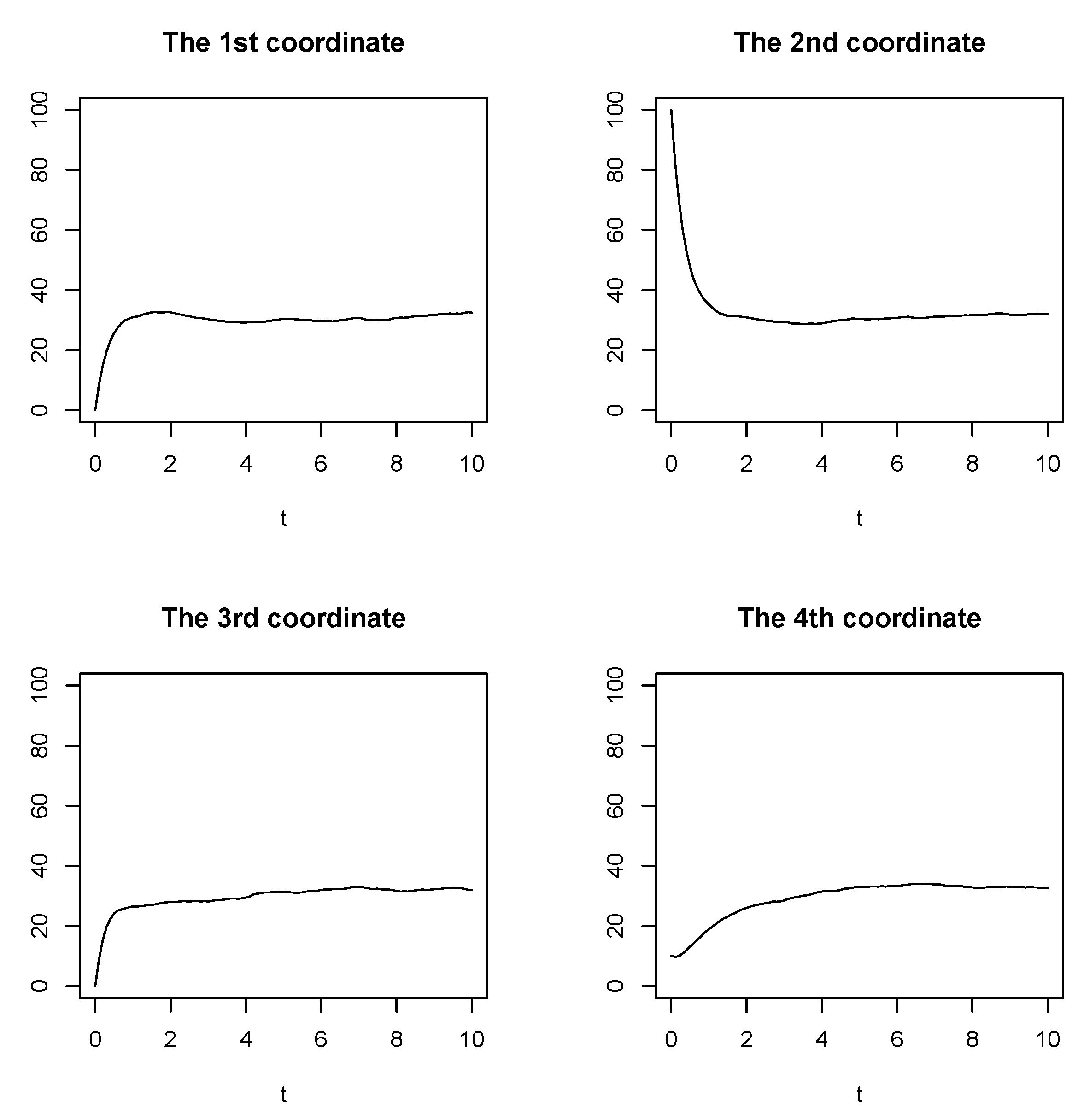
The simulated trajectories in the physical domain of a sample solution to Examples 1 with the non-stationary initial condition and $H=0.75$ are shown in Figure 2.

Example 2.

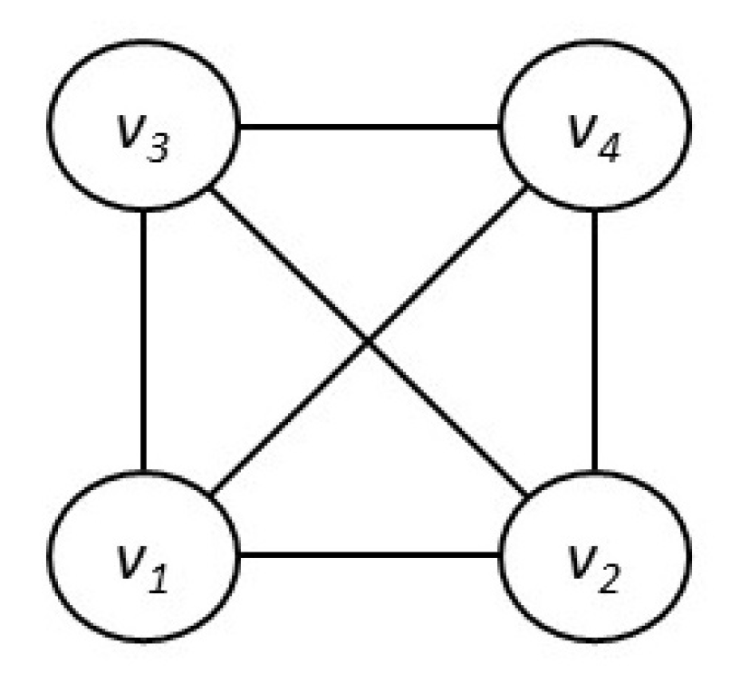
In the second example, we study a stochastic heat Equation (4) on the complete graph shown in Figure 3. Such an equation models situation when the diffusion of heat (or other quantity) occurs between all pairs of vertices.

Simulation setting:

$\lambda =1,\mathsf{\Phi }=Id=diag\{1,1,1,1\},X_0=\left\{\begin{array}{c}(0,100,0,10)\hfill \\ (10,10,10,10)\hfill \end{array}\right.,H=\left\{\begin{array}{c}0.5\hfill \\ 0.75\hfill \end{array}\right.$.

Time step for simulations $\delta t=0.01$, time step for estimation $h=0.1$.

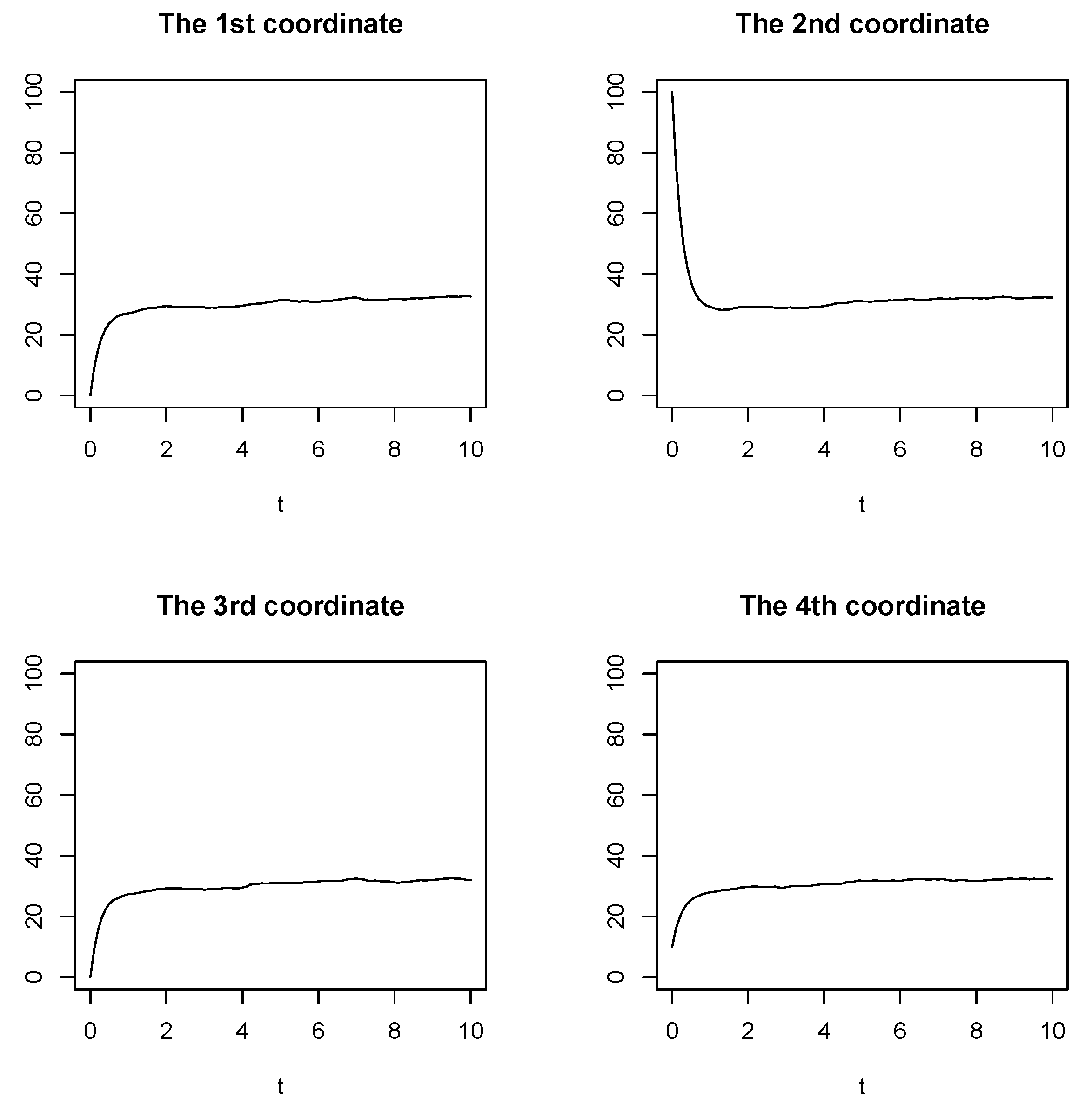
Trajectories of a single realization of the solution to Example (2) with the non-stationary initial condition and $H=0.75$ are depicted in Figure 4.

Example 3.

Consider an evolution equation on N isolated vertices without any interactions (there are no edges) with the drift operator in Equation (5) being a diagonal $N\times N$ matrix:

$$A\left(\lambda \right)=\lambda ·Id=diag\{\lambda ,\lambda ,\dots ,\lambda \}.$$

Such a simple equation is appropriate for studying how the performance of the estimator depends on the number of vertices N.

Simulation setting:

$\lambda =1,\mathsf{\Phi }=Id=diag\{1,1,\dots ,1\},X_0=(0,0,\dots ,0),H=0.75$.

The solutions have been simulated with short time horizon $T=1$ and with time step $\delta t=0.01$. For the purpose of estimating λ, we have sampled the simulated solution with time step $h=0.1$, i.e., we have taken every 10th simulated value.

5.3. Results and Discussion

5.3.1. Examples 1 and 2

The behavior of the combined estimator in different scenarios (various combinations of $X_0$, H, and time horizon T) for the two heat-equation examples is studied below. Besides application of the Formula (32) when $H=0.75$ and (33) when $H=0.5$, we also apply Formula (33) (the MLE criterion when $H=0.5$) for trajectories generated by a model with $H=0.75$. This illustrates the effect of model misspecification when the observed process has fractional noise, but we use the standard estimation technique from white-noise theory.

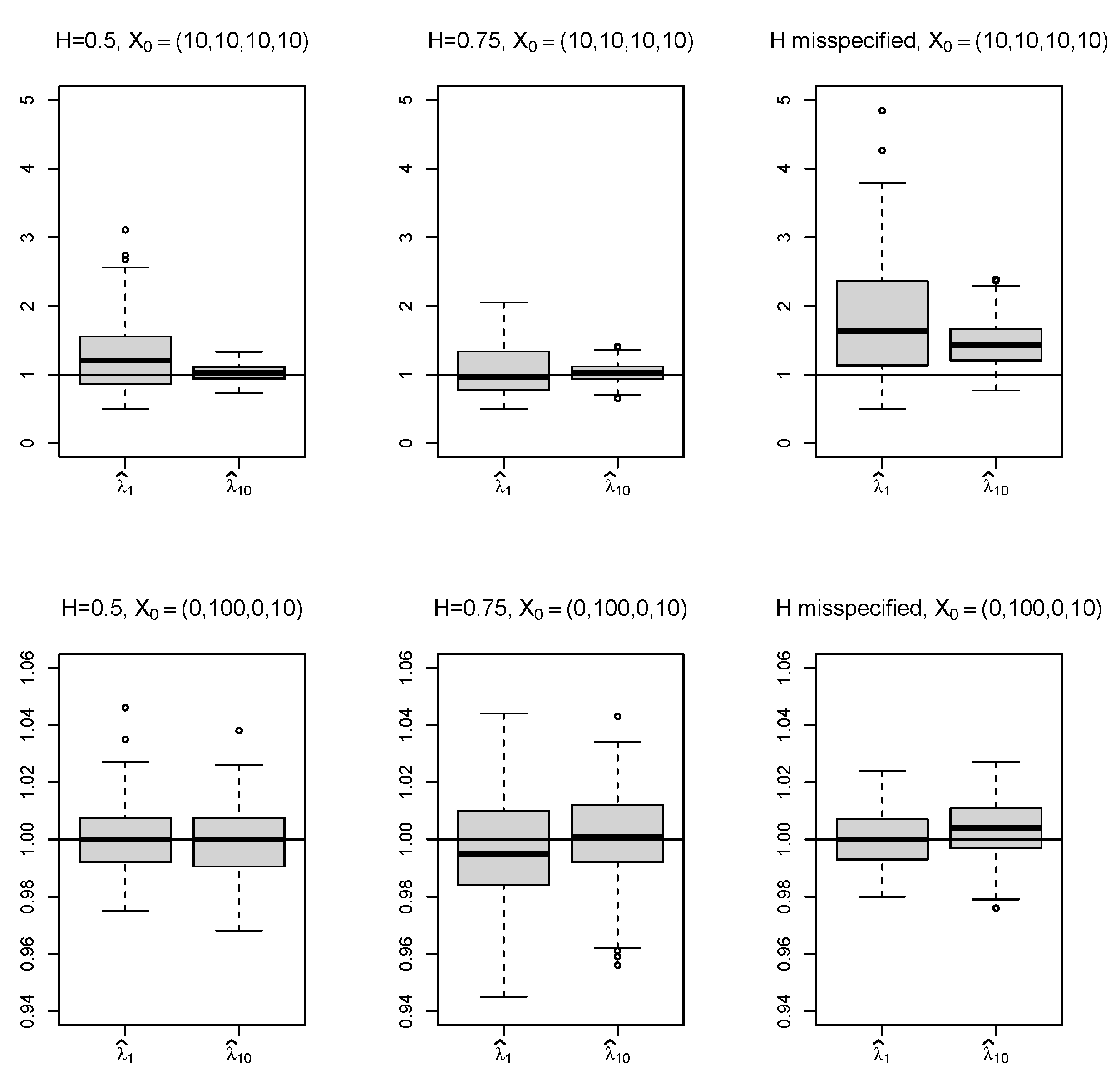
Boxplots of the resulting estimates obtained from the Monte Carlo simulations with 100 independent samples for each scenario are shown in Figure 5 (Example 1) and in Figure 6 (Example 2). The related root mean square errors (RMSE) can be found in

Table 1. RMSE of the calculated estimates using 100 samples with $\lambda =1$.

Initial Condition	T	H	Example 1	Example 2
(0, 100, 0, 10)	1	0.5	0.0132944	0.0126748
(0, 100, 0, 10)	1	0.75	0.0227583	0.0201745
(0, 100, 0, 10)	10	0.5	0.0134145	0.0125359
(0, 100, 0, 10)	10	0.75	0.019374	0.016389
(0, 100, 0, 10)	100	0.75	0.0180549	0.016476
(0, 100, 0, 10)	1	misspecified	0.0118246	0.0101789
(0, 100, 0, 10)	10	misspecified	0.0128522	0.0114258
(10, 10, 10, 10)	1	0.5	1.04229	0.637036
(10, 10, 10, 10)	1	0.75	0.654375	0.396853
(10, 10, 10, 10)	10	0.5	0.215363	0.139379
(10, 10, 10, 10)	10	0.75	0.217963	0.157472
(10, 10, 10, 10)	100	0.75	0.0714899	0.0515372
(10, 10, 10, 10)	1	misspecified	1.46259	1.18714
(10, 10, 10, 10)	10	misspecified	0.461442	0.568978

.

Estimating $\lambda$ from solutions with the non-stationary initial condition provides significantly more accurate results compared to estimating from the stationary solution. This indicates that the combined estimator can efficiently utilize the valuable information about $\lambda$ encoded in the speed of the convergence of the solution process to the stationary state in the initial phase. The solution in this phase is affected mainly by the drift operator; the effect of the random noise is marginal. This is in contrast to the stationary phase, where random noise prevails.

In line with the strong consistency of the combined estimator, we observe that increasing time horizon improves the accuracy of the estimates. This property is evident in the stationary case. In non-stationary case, only minor improvement has been observed, because most of the information about $\lambda$ is stored in initial non-stationary phase. Time horizon T would have to be much longer to surpass this effect.

Analysis of the misspecified model reveals that it provides significantly biased estimates for stationary processes. Hence, there is a strong need to use specific methods for processes with fractional (autocorrelated) noise. The combined estimator overcomes this issue by the correction term for autocorrelation contained in Formula (32), but not in (33). In the non-stationary case, the effect of the initial condition suppresses the effect of the autocorrelated noise and the misspecified estimator shows competitive performance.

Comparison of Example 1 with Example 2 shows slightly better estimates for the latter (in terms of RMSE). More edges in the complete graph in Example 2 represent more transfer paths and more heat diffusion. In result, it contains more information about $\lambda$ within the fixed time-window.

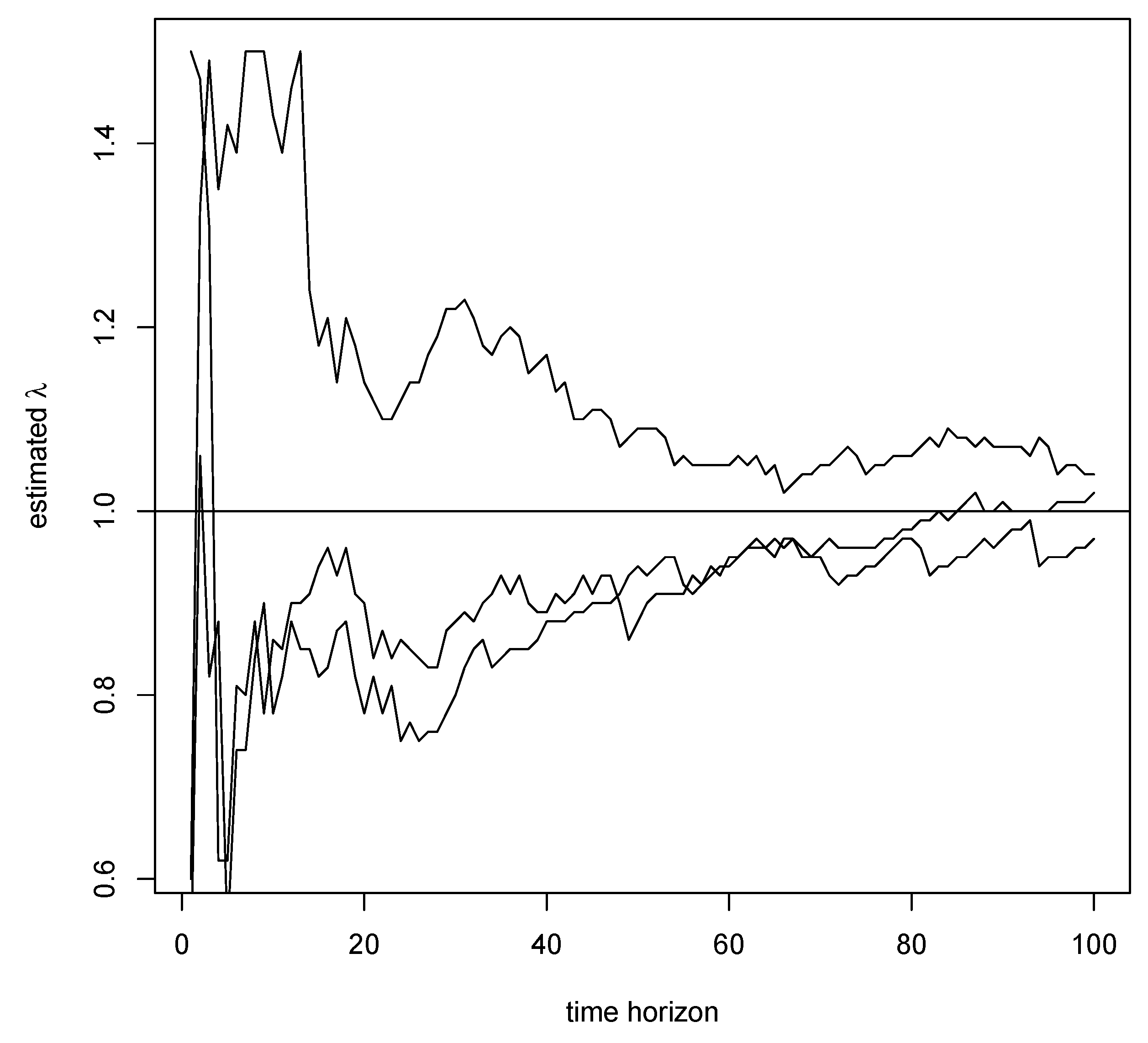
Figure 7 illustrates the path-wise (almost sure) convergence of the estimator to the true value of $\lambda$. It shows the evolution of the estimates with increasing time horizon T for three samples of the solution to Example 1 with $H=0.75$ and $X_0=(10,10,10,10)$.

5.3.2. Example 3

The dependence of the behavior of the combined estimator on the number of vertices in the setting of the diagonal example with no interactions between vertices (Example 3) is studied below.

The results of Monte Carlo simulations (with 100 runs for each setting) are shown in the table with corresponding RMSE (

Table 2. RMSE of the calculated estimates using 100 samples with $\lambda =1$ in Example 3.

N	RMSE
3	0.999612
5	0.756201
10	0.508276
20	0.472542

). Obviously, with an increasing number of vertices, the estimator improves, which suggests the space-consistency of the combined estimator. This consistency can be conjectured due to the fact that the combined estimator follows the maximum likelihood approach in the space domain. However, a detailed study of space asymptotics of the combined estimator is not in the scope of this paper, and may be the direction of the further research. We expect that the asymptotic behavior of eigenvalues of the drift operator $A\left(\lambda \right)$ will play important role here.

6. Conclusions

In this paper, we initiated a study of parameter estimation in the setting of stochastic evolution equations on graphs driven by fractional Brownian motions. We illustrated on the numerical simulation that such models can not be treated directly by estimation techniques known for equations with standard Brownian motion (see the misspecified model). Hence, we introduced a novel approach, which combines the conditional least-squares technique in the time domain with the maximum-likelihood technique in the space domain. This leads to a new estimator that we call the combined estimator. It has favourable asymptotic properties; we proved its strong consistency in the long-span asymptotic regime. Unlike the minimum-contrast estimator studied in [14], which could also be applied in our setting, the combined estimator is very efficient also for non-stationary solutions. We also derived an easy-to-implement formula in diagonal setting and illustrate its behaviour in various scenarios by Monte Carlo simulations.

Although we documented promising properties of the combined estimator above, some important questions remain open and may determine the direction of further research. These include (but are not limited to) the speed of convergence and asymptotic distribution, the space asymptotics (increasing number of nodes), modification for the singular case with Hurst index $H<1/2$ (negatively correlated increments), simultaneous estimation of H, $\mathsf{\Phi }$ (or its magnitude) and $\lambda$, or parameter estimation in more complex and interesting examples with the application of more sophisticated graph theory.

References

1. Mesbahi, M.; Egerstedt, M. Graph Theoretic Methods in Multiagent Networks (Princeton Series in Applied Mathematics); Princeton University Press: Princeton, NJ, USA, 2010. [Google Scholar]
2. Bonaccorsi, S.; Mugnolo, D. Existence of strong solutions for neuronal network dynamics driven by fractional Brownian motions. Stoch. Dyn. 2010, 10. [Google Scholar] [CrossRef] [Green Version]
3. Mishura, Y. Stochastic Calculus for Fractional Brownian Motion and Related Processes; Springer: Berlin/Heidelberg, Germany, 2008. [Google Scholar]
4. Biagini, F.; Hu, Y.; Øksendal, B.; Zhang, T. Stochastic Calculus for Fractional Brownian Motion and Applications; Springer: London, UK, 2008. [Google Scholar]
5. Zhang, Z.; Karniadakis, G.E. Numerical Methods for Stochastic Partial Differential Equations with White Noise; Springer International Publishing AG: Cham, Switzerland, 2017. [Google Scholar] [CrossRef]
6. Kutoyants, Y. Statistical Inference for Ergodic Diffusion Processes; Springer: London, UK, 2004. [Google Scholar]
7. Cialenco, I. Statistical inference for SPDEs: An overview. Stat. Inference Stoch. Process. 2018, 21, 309–329. [Google Scholar] [CrossRef] [Green Version]
8. Kubilius, K.; Mishura, Y.; Ralchenko, K. Parameter Estimation in Fractional Diffusion Models; Springer International Publishing AG: Cham, Switzerland, 2017. [Google Scholar]
9. Prakasa Rao, B.L.S. Statistical Inference for Fractional Diffusion Processes; John Wiley & Sons: Chichester, UK, 2010. [Google Scholar]
10. Estrada, E. d-Path Laplacians and Quantum Transport on Graphs. Mathematics 2020, 8, 527. [Google Scholar] [CrossRef] [Green Version]
11. Markussen, B. Likelihood inference for a discretely observed stochastic partial differential equation. Bernoulli 2003, 9, 745–762. [Google Scholar] [CrossRef]
12. Cialenco, I.; Delgado-Vences, F.; Kim, H. Drift estimation for discretely sampled SPDEs. Stoch. Partial. Differ. Equ. Anal. Comput. 2020. [Google Scholar] [CrossRef] [Green Version]
13. Hildebrandt, F.; Trabs, M. Parameter estimation for SPDEs based on discrete observations in time and space. arXiv 2019, arXiv:1910.01004. [Google Scholar]
14. Kříž, P.; Maslowski, B. Central limit theorems and minimum-contrast estimators for linear stochastic evolution equations. Stochastics 2019, 91, 1109–1140. [Google Scholar] [CrossRef] [Green Version]
15. Kříž, P.; Szała, L. Least-Squares Estimators of Drift Parameter for Discretely Observed Fractional Ornstein-Uhlenbeck Processes. Mathematics 2020, 8, 716. [Google Scholar] [CrossRef]
16. Istas, J.; Lang, G. Quadratic variations and estimation of the local Hölder index of a Gaussian process. Ann. l’Inst. Henri Poincare (B) Probab. Stat. 1997, 33, 407–436. [Google Scholar] [CrossRef] [Green Version]
17. Coeurjolly, J. Hurst exponent estimation of locally self-similar Gaussian processes using sample quantiles. Ann. Stat. 2008, 36, 1404–1434. [Google Scholar] [CrossRef]
18. Rosenbaum, M. Estimation of the volatility persistence in a discretely observed diffusion model. Stoch. Process. Appl. 2008, 118, 1434–1462. [Google Scholar] [CrossRef]
19. Brouste, A.; Iacus, S. Parameter estimation for the discretely observed fractional Ornstein-Uhlenbeck process and the Yuima R package. Comput. Stat. 2013, 28, 1529–1547. [Google Scholar] [CrossRef] [Green Version]
20. Pipiras, V.; Taqqu, M. Integration questions related to fractional Brownian motion. Probab. Theory Relat. Fields 2000, 118, 251–291. [Google Scholar] [CrossRef]
21. Duncan, T.E.; Pasik-Duncan, B.; Maslowski, B. Fractional Brownian motion and stochastic equations in Hilbert spaces. Stoch. Dyn. 2002, 2, 225–250. [Google Scholar] [CrossRef]
22. Pasik-Duncan, B.; Duncan, T.E.; Maslowski, B. Linear stochastic equations in a Hilbert space with a fractional Brownian motion. Int. Ser. Oper. Res. Manag. Sci. 2006, 94, 201–222. [Google Scholar] [CrossRef]
23. Tindel, S.; Tudor, C.; Viens, F. Stochastic evolution equations with fractional Brownian motion. Probab. Theory Relat. Fields 2003, 127, 186–204. [Google Scholar] [CrossRef]
24. Beran, J.; Feng, Y.; Ghosh, S.; Kulik, R. Long-Memory Processes: Probabilistic Properties and Statistical Methods; Springer: Berlin/Heidelberg, Germany, 2013. [Google Scholar]
Figure 1. Stochastic heat equation on a linear graph.
Mathematics 08 01766 g001
Figure 2. The trajectories of a sample solution to Example 1, where H = 0.75 .
Mathematics 08 01766 g002
Figure 3. Stochastic heat equation on a complete graph.
Mathematics 08 01766 g003
Figure 4. The trajectories of a sample solution to Example 2, where H = 0.75 .
Mathematics 08 01766 g004
Figure 5. Boxplots of the estimated λ in Example 1 for time horizons T = 1 (denoted by λ ^ 1 ) and T = 10 (denoted by λ ^ 10 ) calculated for 100 samples in every case considered; the horizontal line shows the true value of the estimated parameter λ = 1 .
Mathematics 08 01766 g005
Figure 6. Boxplots of the estimated λ in Example 2 for time horizons T = 1 (denoted by λ ^ 1 ) and T = 10 (denoted by λ ^ 10 ) calculated for 100 samples in every case considered; the horizontal line shows the true value of the estimated parameter λ = 1 .
Mathematics 08 01766 g006
Figure 7. The convergence of λ ^ for three sample solutions from Example 1 with H = 0.75 and X 0 = ( 10 , 10 , 10 , 10 ) ; the horizontal line shows the true value of the estimated parameter λ = 1 .
Mathematics 08 01766 g007