Numerical Solutions for Multi-Term Fractional Order Differential Equations with Fractional Taylor Operational Matrix of Fractional Integration

Abstract

In this article, we propose a numerical method based on the fractional Taylor vector for solving multi-term fractional differential equations. The main idea of this method is to reduce the given problems to a set of algebraic equations by utilizing the fractional Taylor operational matrix of fractional integration. This system of equations can be solved efficiently. Some numerical examples are given to demonstrate the accuracy and applicability. The results show that the presented method is efficient and applicable.

1. Introduction

Fractional calculus is an emerging field of mathematics, which is a generalisation of differentiation and integration to non-integer orders. The history of fractional calculus is almost as long as the history of classical calculus, beginning with some speculations of Leibniz (1695, 1697) and Euler (1730). However, fractional calculus and fractional differential equations (FDEs) are increasingly becoming popular in recent years. The progressively developing history of this old and yet novel topic can be found in [1,2,3,4,5]. In fact, fractional calculus provides the mathematical modeling of some important phenomena like social and natural in a more powerful way than the classical calculus. During the last few decades, many applications were reported in many branches of science and engineering such as chaotic systems [6,7], fluid mechanics [8], viscoelasticity [9], optimal control problems [10,11], chemical kinetics [12,13], electrochemistry [14], biology [15], physics [16], bioengineering [17], finance [18], social sciences [19], economics [20,21], optics [22], chemical reactions [23], rheology [24], and so on. Due to the importance of FDEs, the solutions of them are attracting widespread interest. On the other hand, analytical solutions are not always possible for solving them. Therefore, numerical techniques becomes more important for solving such equations.

There are various numerical methods have been developed for solving FDEs in literature such as predictor-corrector method [25], Laplace transforms [26], Taylor collocation method [27], variational iteration method and homotopy perturbation method [8] (Chapter 6), Adomian decomposition method [28], Tau method [29], inverse Laplace transform [30], Haar wavelet collocation method [31], generalized block pulse operational matrix [32], shifted Legendre-tau method [33], fractional multi-step differential transformed method [34], q-homotopy analysis transform method [35], conformable Laplace transform [36], fractional B-splines collocation method [37], finite difference method [38], homotopy analysis method [39] and so on.

Multi-term fractional differential equations are one of the most important type of FDEs, which is a system of mixed fractional and ordinary differential equations and involving more than one fractional differential operators. Nowadays, they are widely appearing for modelling of many important processes, especially for multirate systems. Their numerical solution is then a strong subject that deserves high attention. In this paper, motivated by the results reported in [40,41] for solving a smaller class of problems where the highest order of derivative is an integer and involving at most one noninteger order derivative, we go further and establish a method for numerical solutions for higher order and arbitrary multi-term fractional differential equations which have a general form

$$\begin{array}{c}\hfill D^{\alpha }y\left(t\right)=f\left(t,y\left(t\right),D^{{\beta }_0}y\left(t\right),D^{{\beta }_1}y\left(t\right),\dots ,D^{{\beta }_k}y\left(t\right)\right),t\in [0,R]\end{array}$$

(1)

where $D^{\alpha }$ representing the Caputo fractional derivative of order $\alpha >0$ and we assume that $0<{\beta }_0<{\beta }_1<\dots <{\beta }_k<\alpha ,$ $y^{\left(p\right)}=Y_p,$ $p=0,1,\dots n$ where $n-1<\alpha <n.$

Multi-term fractional order differential equations also have useful properties and they can describe complex multi-rate physical processes in a various way and can be applied in many fields, see e.g., [2,4,26,42]. Basset [43] and Bagley–Torvik [44] equations can be given as important examples for smaller class of multi-term fractional differential equations. Existence, uniqueness and stability of solution for multi-term fractional differential equations are discussed in [45,46,47,48,49]. Because of difficulty of finding the exact solutions for such equations, many new numerical techniques have been developed to investigate the numerical solutions such as Adams method [50], Haar wavelet method [51], differential transform method [52], Adams–Bashforth–Moulton method [53], collocation method based on shifted Chebyshev polynomials of the first kind [54], Boubaker polynomials method [55], matrix Mittag–Leffler functions [56], differential transform method [57] and so on.

Our main purpose is to present an effective, reliable method to approximate initial value problem for the Equation (1). In order to reach this aim, we rewrite and focus the general type of Caputo multi-term fractional differential equation given in Equation (1) in the following linear form

$$\begin{array}{cc}\hfill D^{\alpha }y\left(t\right)& =\sum _{i=0}^k{u}_i{D}^{{\beta }_i}y\left(t\right)+u_{k+1}y\left(t\right)+f\left(t\right),0\le t\le R,\hfill \end{array}$$

(2)

subject to the

$$\begin{array}{cc}\hfill y^{\left(p\right)}\left(0\right)& =Y_p,p=0,1,\dots ,n-1\mathrm{where}n-1<\alpha <n\hfill \\ \hfill u_i(i& =0,1,\dots ,k)\mathrm{are}\mathrm{known}\mathrm{coefficients}\mathrm{and}\hfill \\ \hfill 0& <{\beta }_0<{\beta }_1<\dots <{\beta }_k<\alpha \hfill \end{array}$$

(3)

Here, we also state that the highest order $\alpha$ need not to be an integer. This equation is important in applications due to the fact it can treat the problems with fractional force, therefore it is suitable for being treated within fractional operators of Caputo type.

In this work, a numerical approach based on fractional Taylor vector is proposed to solve the initial value problem of general type of multi-term fractional differential equations which is given in Equations (2) and (3). The core idea of this method is to employ the operational matrix of fractional integration based on fractional Taylor vector to given problem and reduce it to a set of algebraic equations which can be efficiently solved.

The structure of the manuscript is organized as follows. In Section 2, we briefly introduce some preliminary ideas of fractional calculus and necessary definitions. In Section 3, an operational matrix of fractional integration based on fractional taylor vector is derived. In Section 4, we present the numerical algorithm to solve the given equation and a pseudo-code for matlab is also provided in Algorithm 1. In Section 5, the presented method is applied to six examples to demonstrate the efficiency. A final conclusion is presented in the last section.

2. Preliminary Knowledge

In this section, we recall some fundamental definitions and preliminary facts of fractional calculus.

2.1. The Fractional Integral and Derivative

Definition 1.

The Riemann–Liouville fractional integral to order α of an integrable function $y\left(t\right)$ is defined to be

$$I^{\alpha }y\left(t\right)=\left\{\begin{array}{cc}{\displaystyle \frac{1}{\Gamma \left(\alpha \right)}{\int }_0^t{(t-s)}^{\alpha -1}y\left(q\right)\mathrm{d}s,}\hfill & \alpha >0\hfill \\ y\left(t\right),\hfill & \alpha =0\hfill \end{array}\right.$$

(4)

When applied to a power function, it yields the following result:

$$I^{\alpha }{\left(t\right)}^c=\frac{\Gamma (c+1)}{\Gamma (c+\alpha +1)}{\left(t\right)}^{c+\alpha },\alpha \ge 0,c>-1$$

(5)

The operator has a semigroup property, namely

$$I^{\alpha }{I}^{\beta }y\left(t\right)=I^{\beta }{I}^{\alpha }y\left(t\right),\alpha ,\beta >0$$

and it is linear, namely

$$I^{\alpha }(A_1{y}_1\left(t\right)+A_2{y}_2\left(t\right))=A_1{I}^{\alpha }{y}_1\left(t\right)+A_2{I}^{\alpha }{y}_2\left(t\right)$$

for any two functions $y_1$,$y_2$ and constants $A_1$,$A_2$.

Definition 2.

The fractional derivative of $y\left(t\right)$ of the order α in the Caputo sense is given as

$$D^{\alpha }y\left(t\right)=I^{j-\alpha }\left(\frac{{\mathrm{d}}^j}{\mathrm{d}{t}^j}y\left(t\right)\right),j-1<\alpha \le j,j\in \mathbb{N}$$

(6)

2.2. Some Properties

• The Riemann-Liouville fractional integral and Caputo fractional derivative do not usually commute with each other. The following Newton–Leibniz identity gives an important relation between them:

  $$I^{\alpha }\left(D^{\alpha }y\left(t\right)\right)=y\left(t\right)-\sum _{i=0}^{j-1}{y}^{\left(i\right)}\left(0\right)\frac{t^i}{i!}$$

  (7)
• The Caputo fractional derivative also has the following substitution identity. If we write $y_1\left(q\right)=y\left(qR\right)$ and $q=t/R$, then

  $$D^{\alpha }y\left(t\right)=\frac{1}{R^{\alpha }}{D}^{\alpha }{y}_1\left(q\right)$$

  (8)

  where $j-1<\alpha \le j,j\in \mathbb{N}$

3. Operational Matrix of Fractional Integration for Fractional Taylor Vector

3.1. Fractional Taylor Basis Vector

We shall make use of the fractional Taylor vector,

$$T_{m\delta }\left(t\right)=\left[1,t^{\delta },t^{2\delta },\dots ,t^{m\delta }\right]$$

(9)

for $m\in \mathbb{N}$ and $\delta >0$ in the work of this paper.

3.2. Approximation of Function

Suppose that $T_{m\delta }\left(t\right)\subset H$, where H is the space of all square integrable functions on the interval $[0,1]$. For any $y\in H$, since $S=span\left\{1,t^{\delta },t^{2\delta },\dots ,t^{m\delta }\right\}$ is a finite dimensional vector space in $H,$ then, y has a unique best approximation $y_{*}\in S,$ so that

$$\forall \widehat{y}\in S,∥y-y_{*}∥\le ∥y-\widehat{y}∥$$

Therefore, the function y is approximated by fractional Taylor vector as following

$$y\simeq y_{*}=\sum _{i=0}^m{c}_i{t}^{i\delta }=C^T{T}_{m\delta }\left(t\right)$$

(10)

where $T_{m\delta }\left(t\right)$ denote the fractional Taylor vector and

$$C^T=[c_0,c_1,c_2,\dots ,c_m]$$

(11)

are the unique coefficients.

3.3. Fractional Taylor Operational Matrix of Integration

By using the property of Riemann-Liouville fractional integral given in Equations (5) and (9), we get

$$\begin{array}{cc}\hfill I^{\alpha }\left(T_{m\delta }\left(t\right)\right)& =\left[\begin{array}{c}\frac{1}{\Gamma (\alpha +1)}{t}^{\alpha },\frac{\Gamma (\delta +1)}{\Gamma (\delta +\alpha +1)}{t}^{\delta +\alpha },\frac{\Gamma (2\delta +1)}{\Gamma (2\delta +\alpha +1)}{t}^{2\delta +\alpha },\dots ,\frac{\Gamma (m\delta +1)}{\Gamma (m\delta +\alpha +1)}{t}^{m\delta +\alpha }\end{array}\right]\hfill \\ \hfill & =t^{\alpha }{M}_{\alpha }{T}_{m\delta }\left(t\right)\hfill \end{array}$$

(12)

where

$$M_{\alpha }=diag\left[\frac{1}{\Gamma (\alpha +1)},\frac{\Gamma (\delta +1)}{\Gamma (\delta +\alpha +1)},\frac{\Gamma (2\delta +1)}{\Gamma (2\delta +\alpha +1)},\dots ,\frac{\Gamma (m\delta +1)}{\Gamma (m\delta +\alpha +1)}\right]$$

denotes the operational matrix of integration.

If we define $G_{\alpha }$ as

$$G_{\alpha }=\left[\frac{1}{\Gamma (\alpha +1)},\frac{\Gamma (\delta +1)}{\Gamma (\delta +\alpha +1)},\frac{\Gamma (2\delta +1)}{\Gamma (2\delta +\alpha +1)},\dots ,\frac{\Gamma (m\delta +1)}{\Gamma (m\delta +\alpha +1)}\right]$$

then, we can rewrite the Equation (10) as

$$I^{\alpha }\left(T_{m\delta }\left(t\right)\right)=t^{\alpha }{G}_{\alpha }\ast T_{m\delta }\left(t\right)$$

(13)

where ∗ denotes the operation of multiplying matrices term by term.

4. The Numerical Algorithm

In this section, to solve the given multi-term fractional differential equation in Equations (2) and (3), we employ the fractional Taylor method. The algorithm of method is given below.

Firstly, by using the transformation $q=t/R$, we replace the variable $t\in [0,R]$ with $q\in [0,1]$. Now, by using Equation (8) in Equation (2), we get

$$\frac{1}{R^{\alpha }}{D}^{\alpha }{y}_1\left(q\right)=\sum _{i=0}^k\frac{1}{R^{{\beta }_i}}{u}_i{D}^{{\beta }_i}{y}_1\left(q\right)+u_{k+1}{y}_1\left(q\right)+f_1\left(q\right),0\le s\le 1$$

(14)

where $f_1\left(q\right)=f\left(qR\right)$ and $y_1\left(q\right)=y\left(qR\right)$. Similar to Equation (10) we approximate the $y_1\left(q\right)$ as

$$y_1\left(q\right)=\sum _{i=0}^m{c}_i{q}^{i\delta }=C^T{T}_{m\delta }\left(q\right)$$

(15)

such that $T_{m\delta }\left(q\right)={[1,q^{\delta },q^{2\delta },\dots ,q^{m\delta }]}^T$ is the fractional Taylor vector and the unique coefficients $C^T$ is given in Equation (11).

Next, applying the Riemann–Liouville fractional integral on both side of (14), we get

$$\begin{array}{cc}\hfill \frac{1}{R^{\alpha }}\left[y_1\left(q\right)-\sum _{j=0}^{n-1}{y}_1^{\left(j\right)}\left(0^{+}\right)\frac{t^j}{j!}\right]& =\sum _{i=0}^k\frac{1}{R^{{\beta }_i}}{u}_i{I}^{\alpha -{\beta }_i}\left[y_1\left(q\right)-\sum _{j=0}^{n_i-1}{y}_1^{\left(j\right)}\left(0^{+}\right)\frac{t^j}{j!}\right]\hfill \\ \hfill & +u_{k+1}{I}^{\alpha }{y}_1\left(q\right)+I^{\alpha }{f}_1\left(q\right)\hfill \end{array}$$

(16)

where $y^{\left(p\right)}\left(0\right)=V_p,$$p=0,1,\dots ,n-1$ where $n_i-1<{\beta }_i<n_i.$

Hence, by substituting initial conditions (3), we get

$$\frac{1}{R^{\alpha }}\left[y_1\left(q\right)\right]=\sum _{i=0}^k\frac{1}{R^{{\beta }_i}}{u}_i{I}^{\alpha -{\beta }_i}\left[y_1\left(q\right)\right]+u_{k+1}{I}^{\alpha }{y}_1\left(q\right)+h_1\left(q\right)$$

(17)

such that $h_1\left(q\right)=I^{\alpha }{f}_1\left(q\right)+\frac{1}{R^{\alpha }}\left({\sum }_{j=0}^{n-1}{V}_j\frac{t^j}{j!}\right)+{\sum }_{i=0}^k\frac{1}{R^{{\beta }_i}}{u}_i{I}^{\alpha -{\beta }_i}\left({\sum }_{j=0}^{n_i-1}{V}_j\frac{t^j}{j!}\right).$

Now, by using the Equation (12), we approximate the fractional order integrals in Equation (17) and we have

$$\begin{array}{cc}\hfill \frac{1}{R^{\alpha }}\left[C^T{T}_{m\delta }\left(q\right)\right]& =\sum _{i=0}^k\frac{1}{R^{{\beta }_i}}{u}_i{C}^T{q}^{\alpha -{\beta }_i}\left(G_{\alpha -{\beta }_i}\ast T_{m\delta }\left(q\right)\right)\hfill \\ \hfill & +u_{k+1}{q}^{\alpha }{C}^T(G_{\alpha }\ast T_{m\delta }\left(q\right))+h_1\left(q\right)\hfill \end{array}$$

(18)

Finally, by taking the collocation points $q_j=j/m$ ($j=0,1,\dots ,m$) in Equation (18), we get $m+1$ linear algebraic equations. This linear system can be solved for the unknown vector $C^T$. Consequently, $y_1\left(q\right)$ can be approximated by Equation (15).

MATLAB Implementation of Method

The pseudocode given in Algorithm 1 below allows us to use proposed method in MATLAB for obtain a numerical solution of given problem [58].

Algorithm 1: Fractional Taylor Method

[$A,b$] = $fractionalTaylor$($alpha$, $beta$, $Uk$, $func$, $t0$, R, $y0$, m, $delta$)

% Input % $alpha$ is the highest order of fractional derivative of given equation % $beta$ is the order of fractional derivatives other than alpha. $beta$ must be a vector with decending ordered values % $Uk$ is the vector of coefficients % $func$ is defining the right hand side of given problem % $t0$ and R denotes the left and right endpoints % $y0$ is the initial conditions % m denotes the number of steps % $delta$ is a real number greater than zero. We usually take $delta=1$ or $delta=$ fractional part of $alpha$

% Output % A is an $(m+1)$ x $(m+1)$ matrix % b is an $(m+1)$ x 1 matrix

% using $fractionalTaylor.m$, where command $fractionalTaylor.m$ is defined by the Equation (18), gives us the linear system $AC=B$ which is $(m+1)$

% algebraic equations with unknown coefficients $C^T$

% Next step is to use matlab function $linsolve(A,b)$ to solve obtained algebraic equation for unknown coefficient vector $C^T$ with dimension $(m+1)$.

$C=linsolve(A,b)$

% Output % C is an $(m+1)$ x 1 matrix which is the solution of linear system $AC=B$

% Next step is substituting obtained coefficients to $approxSoln\left(\right)$ as input, where the command $approxSoln\left(\right)$ defined by Equation (15), we get the approximate solution of given problem [$s,y$] = $approxSoln\left(C\right)$

% Input % C is the vector of coefficients obtained in previous step.

% Output % s is the nodes on $[t0,R]$ in which the approximate solution calculated % y is the numerical solution evaluated in the points of s.

5. Illustrative Examples

To illustrate the applicability and effectiveness of the presented method, we give six examples in this section. In each example, we apply the fractional Taylor operational matrix method which is presented in previous section and the approximate results compared with analytical solutions. Obtained results indicate that the proposed technique is very effective for multi-term fractional differential equations. In order to solve the numerical computations, MATLAB version R2015a has been used.

For choosing $\delta$, we usually take either $\delta =1$ or $\delta =\alpha -⌊\alpha ⌋$, the fractional part of $\alpha$.

5.1. Example 1

Consider the following form of multi-order fractional differential equation [59]

$$\begin{array}{cc}\hfill D^{\alpha }y\left(t\right)& =u_0{D}^{{\beta }_0}y\left(t\right)+u_1{D}^{{\beta }_1}y\left(t\right)+u_2{D}^{{\beta }_2}y\left(t\right)+u_3{D}^{{\beta }_3}y\left(t\right)+f\left(t\right),0\le t\le R,\hfill \\ \hfill y\left(0\right)& =V_0,y^{\prime }\left(0\right)=V_1\hfill \end{array}$$

(19)

We let $\alpha =2,V_0=V_1=0,R=1,$ the coefficients $u_0=u_2=-1,u_1=2,u_3=0$ and ${\beta }_0=0,{\beta }_1=1,{\beta }_2=\frac{1}{2}$ and the function $f\left(t\right)$ is

$$f\left(t\right)=t^7+\frac{2048}{429\sqrt{\pi }}{t}^{6.5}-14t^6+42t^5-t^2-\frac{8}{3\sqrt{\pi }}{t}^{1.5}+4t-2.$$

where the exact solution is $y\left(t\right)=t^7-t^2.$

We apply the given procedure which is implemented in previous section for solving the Equation (19) step by step.

Firstly, change variable $t\in [0,R]$ to $q\in [0,1]$ by using $q=t/R.$

Now, we use the Equation (8) and get

$$\frac{1}{R^{\alpha }}{D}^{\alpha }{y}_1\left(q\right)=\frac{u_0}{R^{{\beta }_0}}{D}^{{\beta }_0}{y}_1\left(q\right)+\frac{u_1}{R^{\beta 1}}{D}^{{\beta }_1}{y}_1\left(q\right)+\frac{u_2}{R^{{\beta }_2}}{D}^{{\beta }_2}{y}_1\left(q\right)+\frac{u_3}{R^{{\beta }_3}}{D}^{{\beta }_3}{y}_1\left(q\right)+f_1\left(q\right)$$

(20)

where $0\le q\le 1$.

Next, using Equation (7) we get

$$\begin{array}{cc}\hfill \frac{1}{R^{\alpha }}(y_1\left(q\right)-y_1\left(0\right)-q{y}_1\prime \left(0\right))& =\frac{u_0}{R^{{\beta }_0}}{I}^{\alpha -{\beta }_0}(y_1\left(q\right)-y_1\left(0\right)-q{y}_1\prime \left(0\right))\hfill \\ \hfill & +\frac{u_1}{R^{\beta 1}}{I}^{\alpha -{\beta }_1}(y_1\left(q\right)-y_1\left(0\right)-q{y}_1\prime \left(0\right))\hfill \\ \hfill & +\frac{u_2}{R^{{\beta }_2}}{I}^{\alpha -{\beta }_2}(y_1\left(q\right)-y_1\left(0\right)-q{y}_1\prime \left(0\right))\hfill \\ \hfill & +\frac{u_3}{R^{{\beta }_3}}{I}^{\alpha -{\beta }_3}(y_1\left(q\right)-y_1\left(0\right)-q{y}_1\prime \left(0\right))\hfill \\ \hfill & +I^{\alpha }{f}_1\left(q\right).\hfill \end{array}$$

(21)

Now, using Equation (21) and substituting initial conditions $y\left(0\right)=V_0,$ $y^{\prime }\left(0\right)=V_1$ into equation

$$\begin{array}{cc}\hfill \frac{1}{R^{\alpha }}(C^T{T}_{m\delta }\left(q\right)-V_0-Rq{V}_1)& =\frac{u_0}{R^{{\beta }_0}}{I}^{\alpha -{\beta }_0}(C^T{T}_{m\delta }\left(q\right)-V_0-Rq{V}_1)\hfill \\ \hfill & +\frac{u_1}{R^{\beta 1}}{I}^{\alpha -{\beta }_1}(C^T{T}_{m\delta }\left(q\right)-V_0-Rq{V}_1)\hfill \\ \hfill & +\frac{u_2}{R^{{\beta }_2}}{I}^{\alpha -{\beta }_2}(C^T{T}_{m\delta }\left(q\right)-V_0-Rq{V}_1)\hfill \\ \hfill & +\frac{u_3}{R^{{\beta }_3}}{I}^{\alpha -{\beta }_3}(C^T{T}_{m\delta }\left(q\right)-V_0-Rq{V}_1)\hfill \\ \hfill & +I^{\alpha }{f}_1\left(q\right).\hfill \end{array}$$

(22)

From Equation (12), we have

$$\begin{array}{cc}\hfill & \frac{1}{R^{\alpha }}(C^T{T}_{m\delta }\left(q\right)-V_0-Rq{V}_1)\hfill \\ \hfill & =\frac{u_0}{R^{{\beta }_0}}{q}^{\alpha -{\beta }_0}{C}^T(G_{\alpha -{\beta }_0}\ast T_{m\delta }\left(q\right))-\frac{u_0{q}^{\alpha -{\beta }_0}}{R^{{\beta }_0}\Gamma (\alpha -{\beta }_0+1)}{V}_0-\frac{u_0{q}^{\alpha -{\beta }_0+1}}{R^{{\beta }_0}\Gamma (\alpha -{\beta }_0+2)}{V}_1\hfill \\ \hfill & +\frac{u_1}{R^{\beta 1}}{q}^{\alpha -{\beta }_1}{C}^T(G_{\alpha -{\beta }_1}\ast T_{m\delta }\left(q\right))-\frac{u_1{q}^{\alpha -{\beta }_1}}{R^{{\beta }_1}\Gamma (\alpha -{\beta }_1+1)}{V}_0-\frac{u_1{q}^{\alpha -{\beta }_1+1}}{R^{\beta 1}\Gamma (\alpha -{\beta }_1+2)}{V}_1\hfill \\ \hfill & +\frac{u_2}{R^{{\beta }_2}}{q}^{\alpha -{\beta }_2}{C}^T(G_{\alpha -{\beta }_2}\ast T_{m\delta }\left(q\right))-\frac{u_2{q}^{\alpha -{\beta }_2}}{R^{{\beta }_2}\Gamma (\alpha -{\beta }_2+1)}{V}_0-\frac{u_2{q}^{\alpha -{\beta }_2+1}}{R^{{\beta }_2}\Gamma (\alpha -{\beta }_2+2)}{V}_1\hfill \\ \hfill & +\frac{u_3}{R^{{\beta }_3}}{q}^{\alpha -{\beta }_3}{C}^T(G_{\alpha -{\beta }_3}\ast T_{m\delta }\left(q\right))-\frac{u_3{q}^{\alpha -{\beta }_3}}{R^{{\beta }_3}\Gamma (\alpha -{\beta }_3+1)}{V}_0-\frac{u_3{s}^{\alpha -{\beta }_3+1}}{R^{{\beta }_3}\Gamma (\alpha -{\beta }_3+2)}{V}_1\hfill \\ \hfill & +I^{\alpha }{f}_1\left(q\right).\hfill \end{array}$$

(23)

Now, taking $R=1$ in Equation (23) and putting the given values for $V_0,V_1,u_i,{\beta }_i$ where $i=0,1,2,3$ into this equation, we get

$$C^T{T}_{m\delta }=2q^1{C}^T(G_1\ast T_{m\delta }\left(q\right))-q^{3/2}{C}^T(G_{3/2}\ast T_{m\delta }\left(q\right))-q^2{C}^T(G_1\ast T_{m\delta }\left(q\right))+I^2{f}_1\left(q\right)$$

(24)

Finally, taking the collocation points $q_j=j/m$ ($j=0,1,\dots ,m$) generates a linear algebraic system of dimension $m+1$ with unknown vector $C^T$. In order to solve this system by using presented method and comparing the results, we choose $\delta =1$ and different values of m.

To show the efficiency, we compared the numerical results with the method given in [59].

Table 1. The comparison absolute errors of the present scheme and method given in [59] with $m=4,6,7$.

t	Present Method	Method in [59]	Present Method	Method in [59]	Present Method	Method in [59]
	$\mathit{m}=\mathbf{4}$	$\mathit{m}=\mathbf{4}$	$\mathit{m}=\mathbf{6}$	$\mathit{m}=\mathbf{6}$	$\mathit{m}=\mathbf{7}$	$\mathit{m}=\mathbf{7}$
0.2	0.0116	0.0844	6.81430698097618 × 10${}^{-7}$	0.0044	1.040834086 × 10${}^{-16}$	2.81025203108243 × 10${}^{-15}$
0.4	0.0032	0.3501	1.01100805164899 × 10${}^{-4}$	0.0079	2.498001805 × 10${}^{-16}$	6.63358257213531 × 10${}^{-15}$
0.6	0.0108	0.6734	1.2907314422994 × 10${}^{-5}$	0.0143	1.665334537 × 10${}^{-16}$	3.27515792264421 × 10${}^{-15}$
0.8	0.0037	1.0234	1.16246682382747 × 10${}^{-4}$	0.0214	3.330669074 × 10${}^{-16}$	4.25770529943748 × 10${}^{-14}$
1.0	0.0026	1.6700	1.11299947542775 × 10${}^{-5}$	0.0280	1.110223025 × 10${}^{-16}$	2.43819897540083 × 10${}^{-13}$

, compares the obtained results for absolute error with $m=4,6,7$. We observe from Table 1 that, the absolute errors for presented method are smaller and the numerical solution is more accurate for the same size of m.

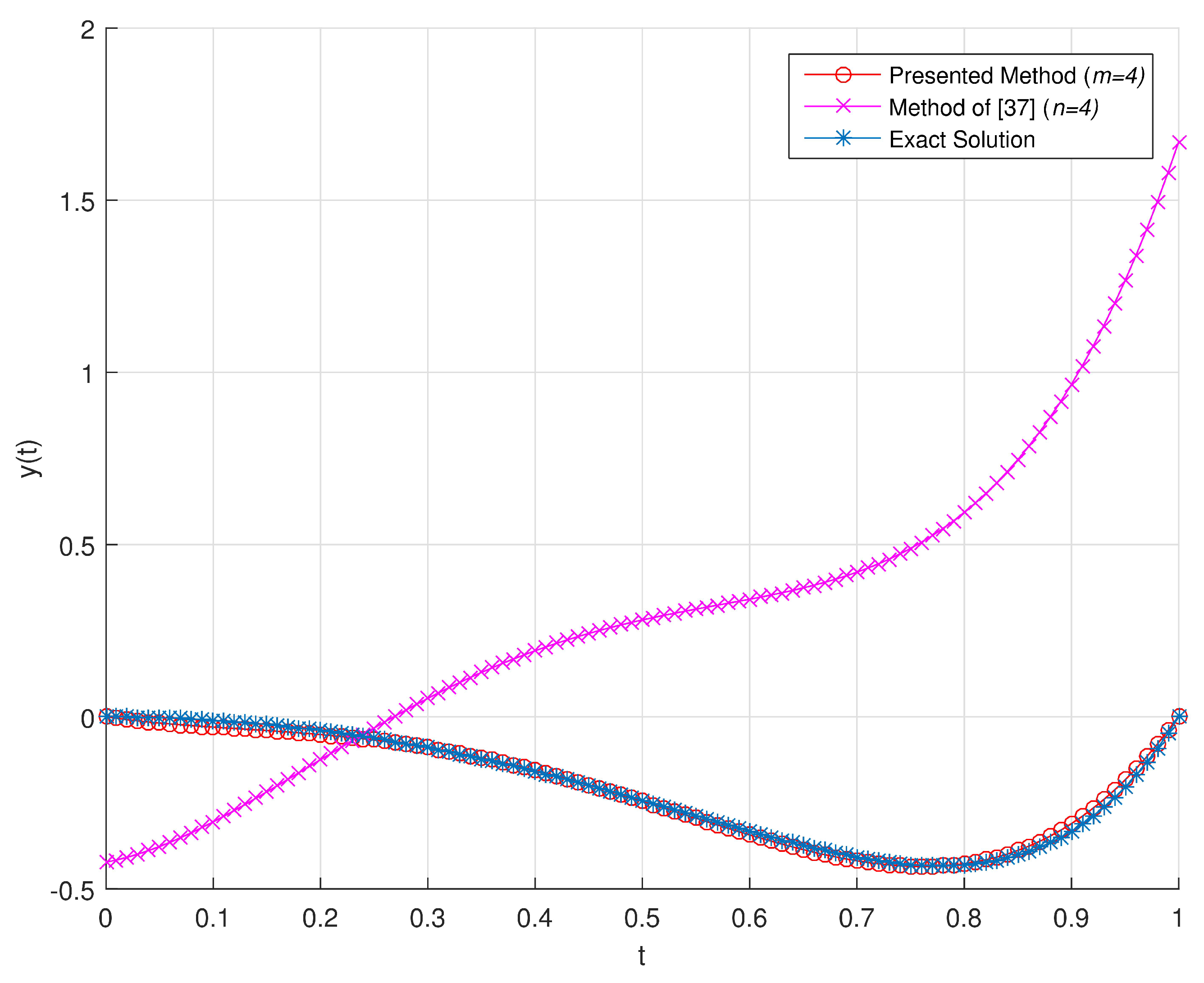
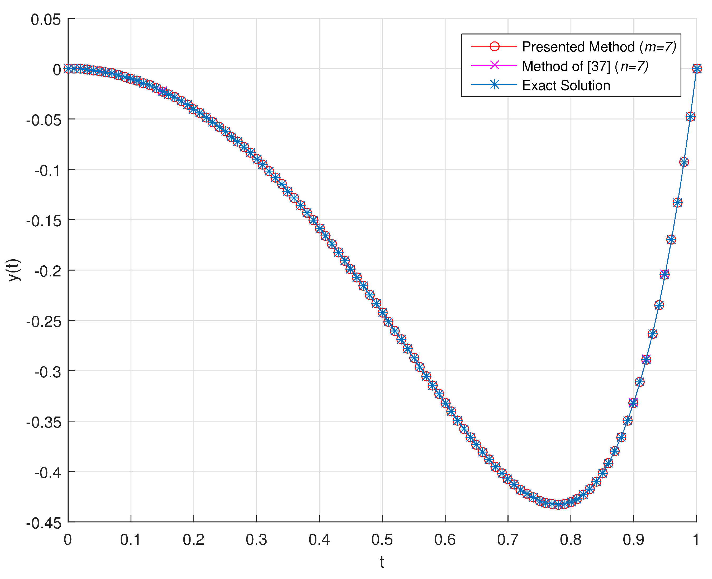
In Figure 1, Figure 2 and Figure 3, we present the graphical representation of comparison between exact solution and the numerical solutions obtained by proposed method and the method of [59] for the problem (19) with $m=4,6,7$ respectively. From these results, we can conclude that $m=4$ and $m=6$ give larger absolute error, while $m=7$ gives smaller absolute error (${10}^{-16}$) and more precise numerical solution. These comparisons also shows that the results obtained by proposed method is closer to the exact solution than the results of [59].

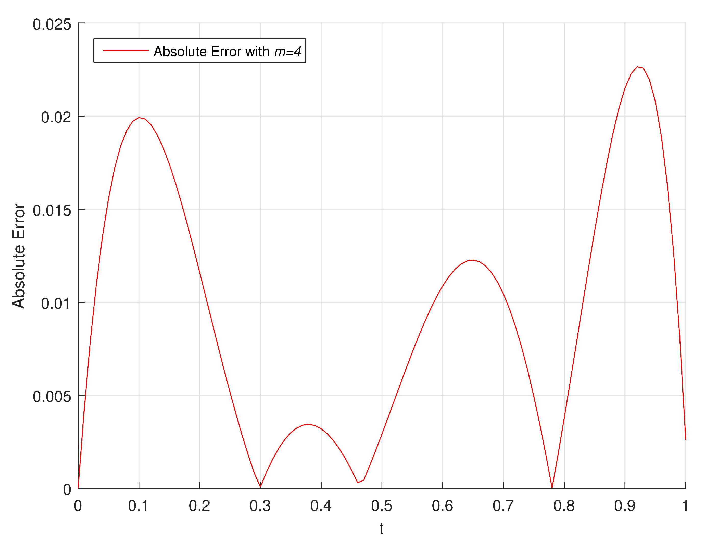
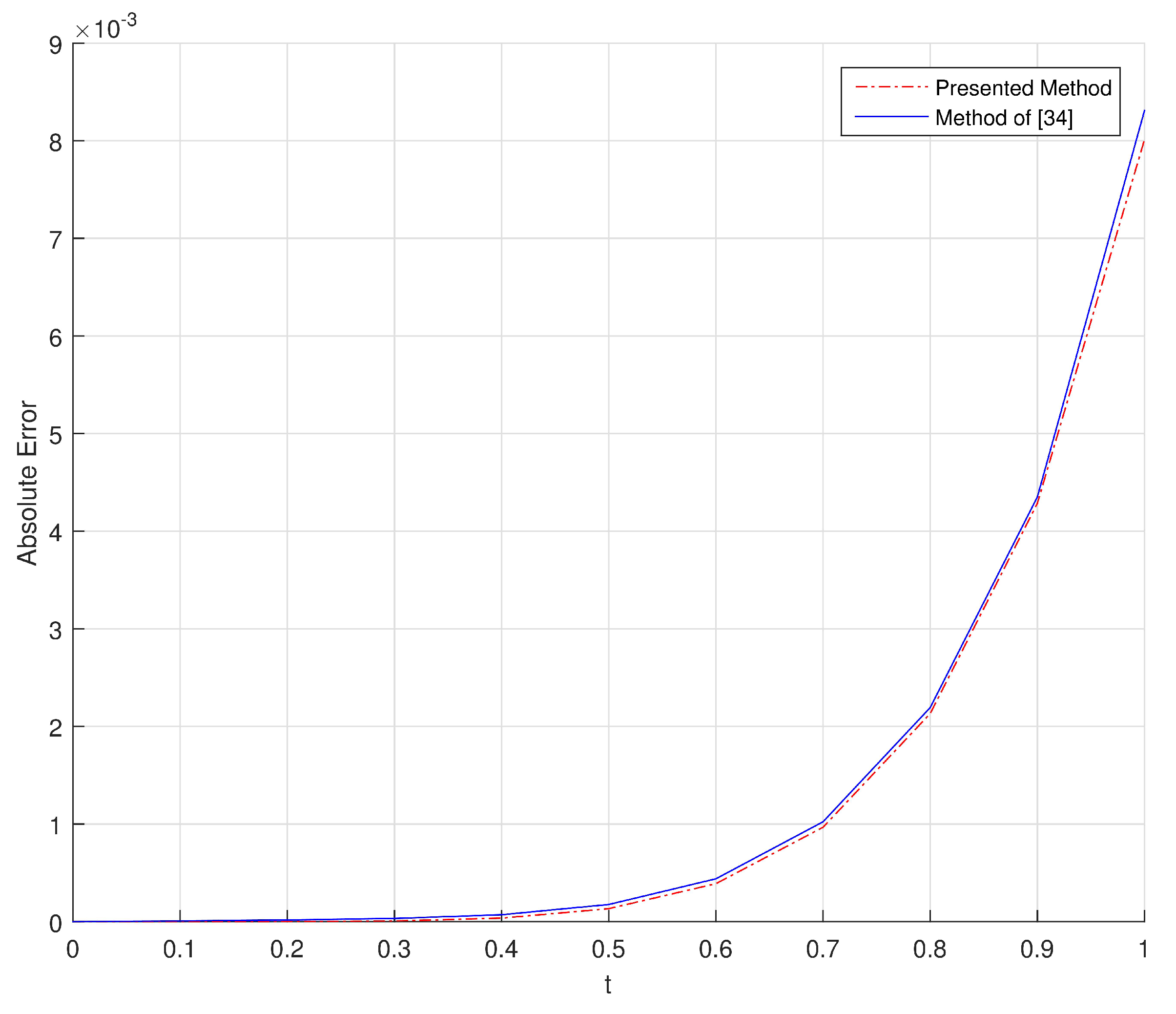
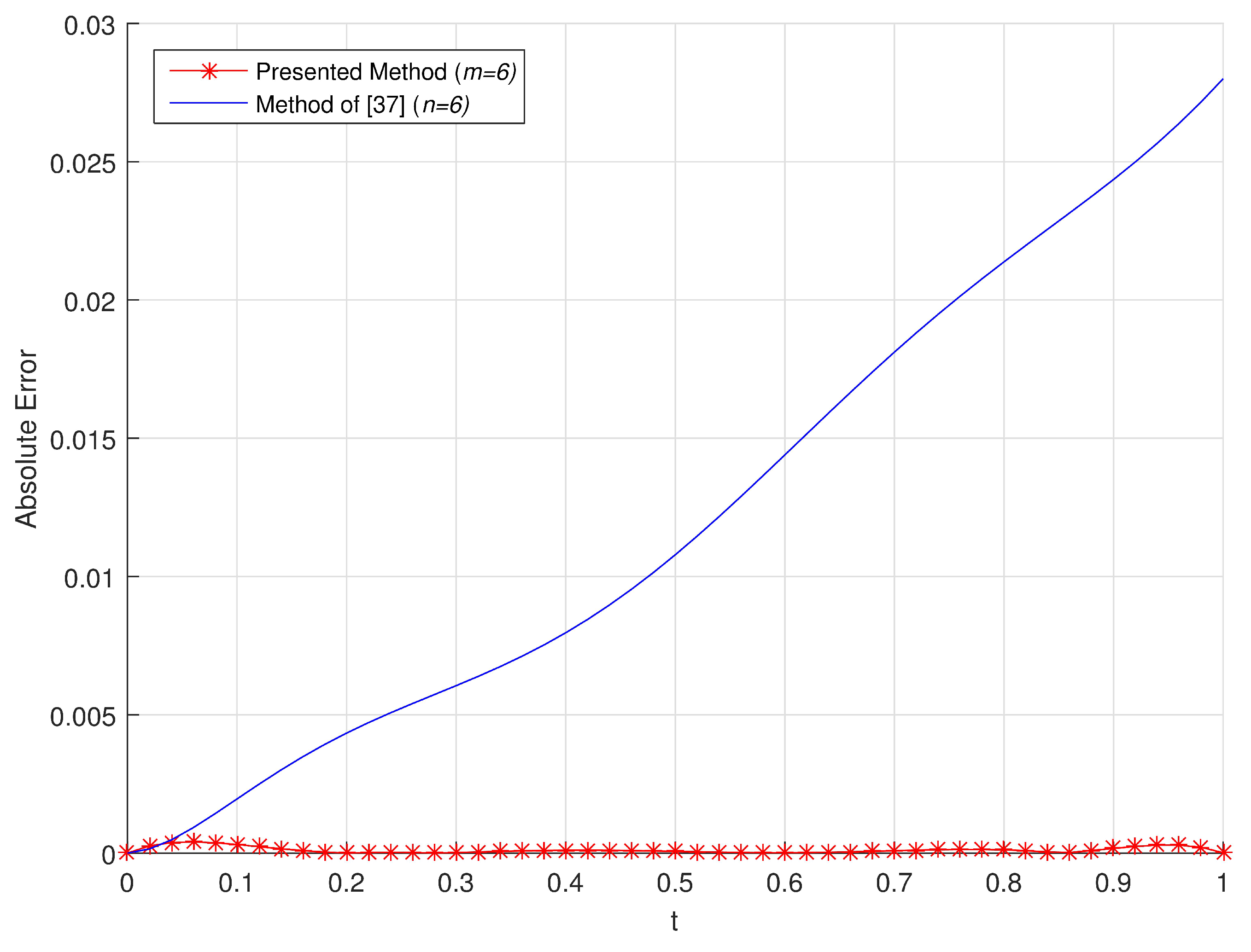
In Figure 4, we show the graphical representation of absolute errors obtained by using proposed method and the method of [59] with $m,n=6$.

From Figure 4, we can conclude that the absolute error obtained by our method is remaining smaller and stable while the absolute error of other method is increasing in the interval $[0,1]$.

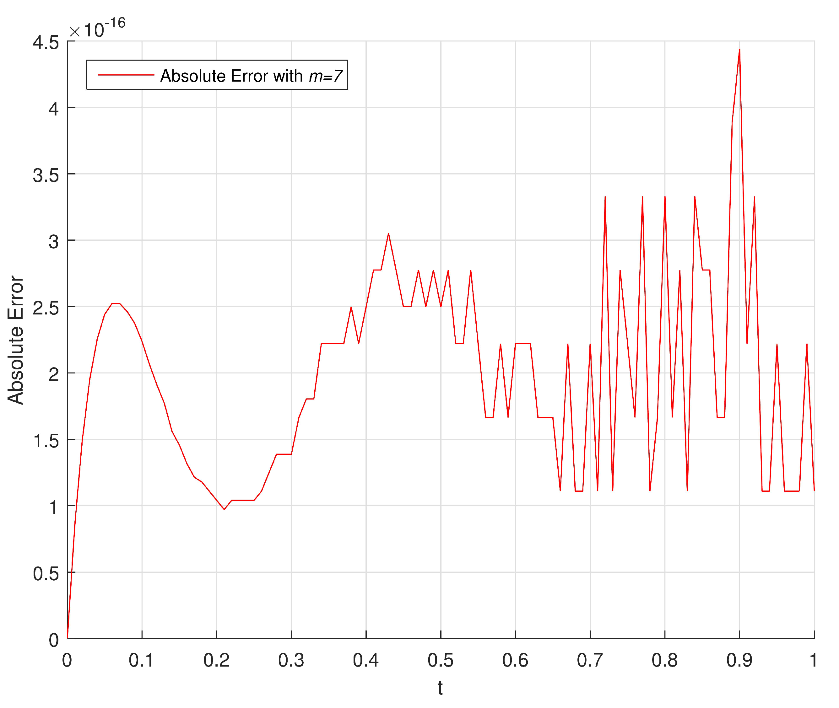
In Figure 5 and Figure 6, we give the graphical representation of absolute errors obtained by using proposed method with $m=4,7$ respectively.

A pseudo-code for MATLAB implementation of Example 1 is given in Algorithm 2 below:

Algorithm 2: Fractional Taylor Method

$alpha=2$;

$beta=[1,1/2,0]$;

$Uk=[2,-1,-1]$;

$func=$@(t) $t^7+2048/(429\ast sqrt\left(pi\right))\ast t^{6.5}-14\ast t^6+42\ast t^5-t^2-\dots$

$8/(3\ast sqrt\left(pi\right))\ast t^{1.5}+4\ast t-2$;

$t0=0$; $R=1$;

$y0=[0;0]$;

$m=4$;

$delta=1$;

$[A,b]=fractionalTaylor$($alpha$, $beta$, $Uk$, $func$, $t0$, R, $y0$, m, $delta$)

$C=linsolve(A,b)$

$[s,y]=approxSoln\left(C\right)$

5.2. Example 2

In this example, we consider the Equation (19) with $\alpha =2,V_0=V_1=0,$ the coefficients $u_0=u_2=-1,u_1=0,u_3=2$ and ${\beta }_0=0,{\beta }_2=\frac{2}{3},{\beta }_3=\frac{5}{3}$ and the function is

$$f\left(t\right)=t^3+6t-\frac{12}{\Gamma \left(\frac{7}{3}\right)}{t}^{\frac{4}{3}}+\frac{6}{\Gamma \left(\frac{10}{3}\right)}{t}^{\frac{7}{3}}.$$

The exact solution of this equation is $y\left(t\right)=t^3$ [59].

Applying the same procedure to given problem as presented in Example 1, we get the following equation

$$\begin{array}{cc}\hfill C^T{T}_{m\delta }& =2q^{1/3}{C}^T(G_{1/3}\ast T_{m\delta }\left(q\right))-q^{4/3}{C}^T(G_{4/3}\ast T_{m\delta }\left(q\right))-q^2{C}^T(G_2\ast T_{m\delta }\left(q\right))+I^2{f}_1\left(q\right)\hfill \end{array}$$

(25)

As we stated in previous example, collocating this equation at the nodes $q_j=j/m$ ($j=0,1,\dots ,m$) generates a system of algebraic equations. In this example, to solve this sysem for $C^T$, we choose $\delta =1,1.5$ and different values of m.

Table 2. The absolute errors with m = 2, 3.

t	$\mathit{\delta }\mathbf{=}\mathbf{1}$, $\mathit{m}\mathbf{=}\mathbf{2}$	$\mathit{\delta }\mathbf{=}\mathbf{1.5}$, $\mathit{m}\mathbf{=}\mathbf{2}$	$\mathit{\delta }\mathbf{=}\mathbf{1}$, $\mathit{m}\mathbf{=}\mathbf{3}$
0	0	0	0
0.1	0.010209105	1.3 × 10${}^{-17}$	7.42 × 10${}^{-17}$
0.2	0.008778787	4.68 × 10${}^{-17}$	1.232 × 10${}^{-16}$
0.3	0.001709047	1.11 × 10${}^{-16}$	1.769 × 10${}^{-16}$
0.4	0.005000117	2.082 × 10${}^{-16}$	2.637 × 10${}^{-16}$
0.5	0.005348703	3.608 × 10${}^{-16}$	4.163 × 10${}^{-16}$
0.6	0.006663287	5.829 × 10${}^{-16}$	6.661 × 10${}^{-16}$
0.7	0.037035855	8.882 × 10${}^{-16}$	9.992 × 10${}^{-16}$
0.8	0.091769001	1.2212 × 10${}^{-15}$	1.5543 × 10${}^{-15}$
0.9	0.176862723	1.6653 × 10${}^{-15}$	1.9984 × 10${}^{-15}$
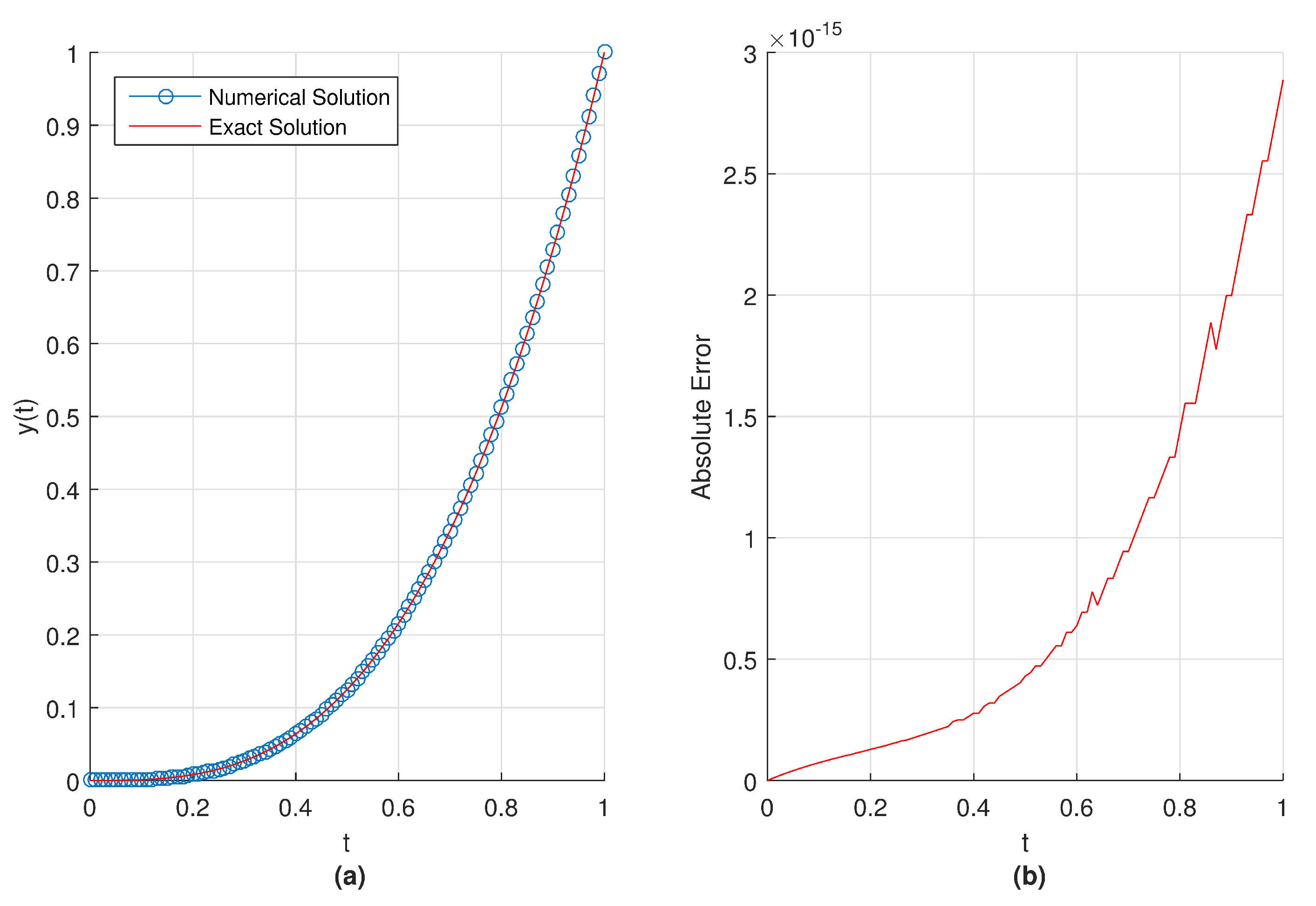
1.0	0.2983170221	2.2204 × 10${}^{-15}$	2.8866 × 10${}^{-15}$

shows the results for obtained absolute errors by using presented method with $m=2,3$. From these results, we can see that, there is satisfactory agreement between the exact solution and numerical solutions. The absolute error is achieved about ${10}^{-15}$. We also note that, the proposed method gives better results for $m=2$ by taking $\delta =1.5$.

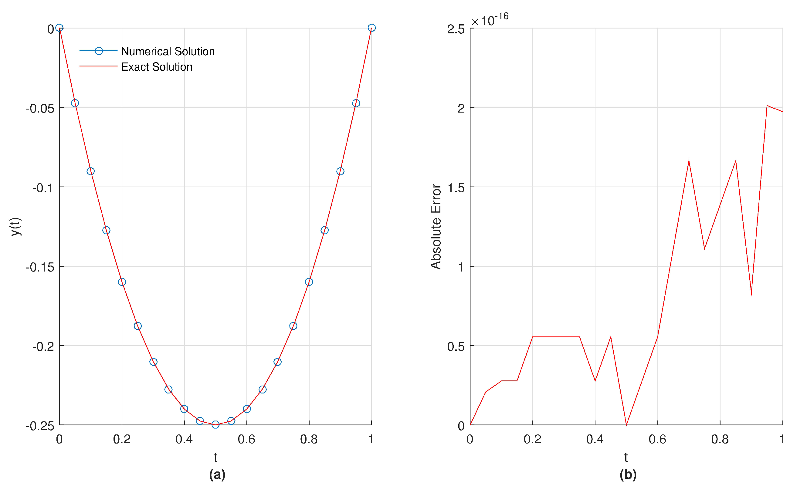
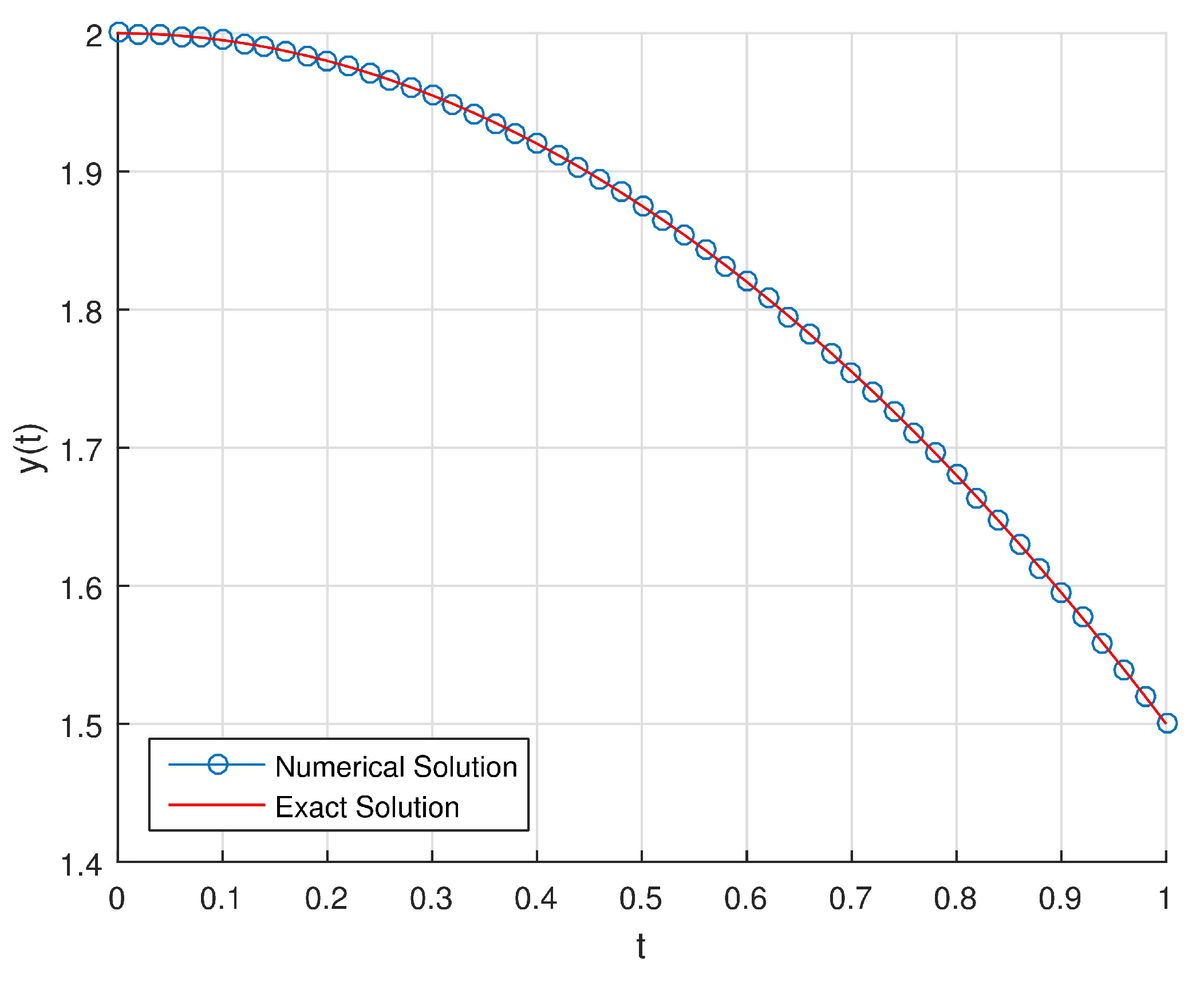
In Figure 7a, we show the graphical representation of obtained numerical solution and the exact solution of the given problem. Figure 7b presents the obtained absolute error by using proposed method with $m=3$.

5.3. Example 3

Consider the multi-term fractional order initial value problem [54]

$$D^{\left(2.2\right)}y\left(t\right)+1.3D^{\left(1.5\right)}y\left(t\right)+2.6y\left(t\right)=sin\left(2t\right),$$

(26)

with initial conditions

$$y\left(0\right)=y^{\prime }\left(0\right)=y^{″}\left(0\right)=0,$$

where the equation have the series solution given by [52]

$$\begin{array}{cc}\hfill y_s\left(t\right)& =\frac{\mathrm{28,561}}{\mathrm{3,600,000}}{t}^6+\frac{2}{\Gamma \left(4.2\right)}{t}^{3.2}-\frac{13}{5\Gamma \left(4.9\right)}{t}^{3.9}+\frac{169}{50\Gamma \left(5.6\right)}{t}^{4.6}\hfill \\ \hfill & -\frac{8}{\Gamma \left(6.2\right)}{t}^{5.2}-\frac{2197}{500\Gamma \left(6.3\right)}{t}^{5.3}-\frac{26}{5\Gamma \left(6.4\right)}{t}^{5.4}+\frac{52}{5\Gamma \left(6.9\right)}{t}^{5.9}.\hfill \end{array}$$

(27)

In order to solve this problem, we choose $\delta =1,$ and $m=10.$

We give the comparison of series solution and the numerical solution obtained by presented method in

Table 3. Comparison of numerical solution with series solution for Example 3.

t	Series Solution [52]	Present Method $\mathit{m}\mathbf{=}\mathbf{10}$
0.0	0	0
0.1	0.000147766	0.000147731
0.2	0.001274983	0.001275552
0.3	0.00439917	0.00440567
0.4	0.010405758	0.010441315
0.5	0.019962077	0.020094648
0.6	0.033452511	0.033841301
0.7	0.050923716	0.051890573
0.8	0.0720381	0.074169634
0.9	0.096035415	0.100321388

.

Table 4. Comparison of absolute errors for Example 3.

t	Present Method $\mathit{m}\mathbf{=}\mathbf{10}$	Method in [54] $\mathit{m}\mathbf{=}\mathbf{20}$
0.0	0	0
0.1	3.47449 × 10${}^{-8}$	5.2560 × 10${}^{-7}$
0.2	5.69366 × 10${}^{-7}$	1.7150 × 10${}^{-6}$
0.3	6.49968 × 10${}^{-6}$	8.2260 × 10${}^{-6}$
0.4	3.55576 × 10${}^{-5}$	3.7820 × 10${}^{-5}$
0.5	0.000132571	0.0001353
0.6	0.00038879	0.000392
0.7	0.000966858	0.0009704
0.8	0.002131534	0.002135
0.9	0.004285973	0.00429

compares the obtained absolute errors by using presented method with the results of [54]. From this compared results, it can be seen that the approximate solution is very close to series solution for a small number of m for the given method.

From the compared results of Table 4, we can conclude that the proposed method has better approach to series solution with a smaller m.

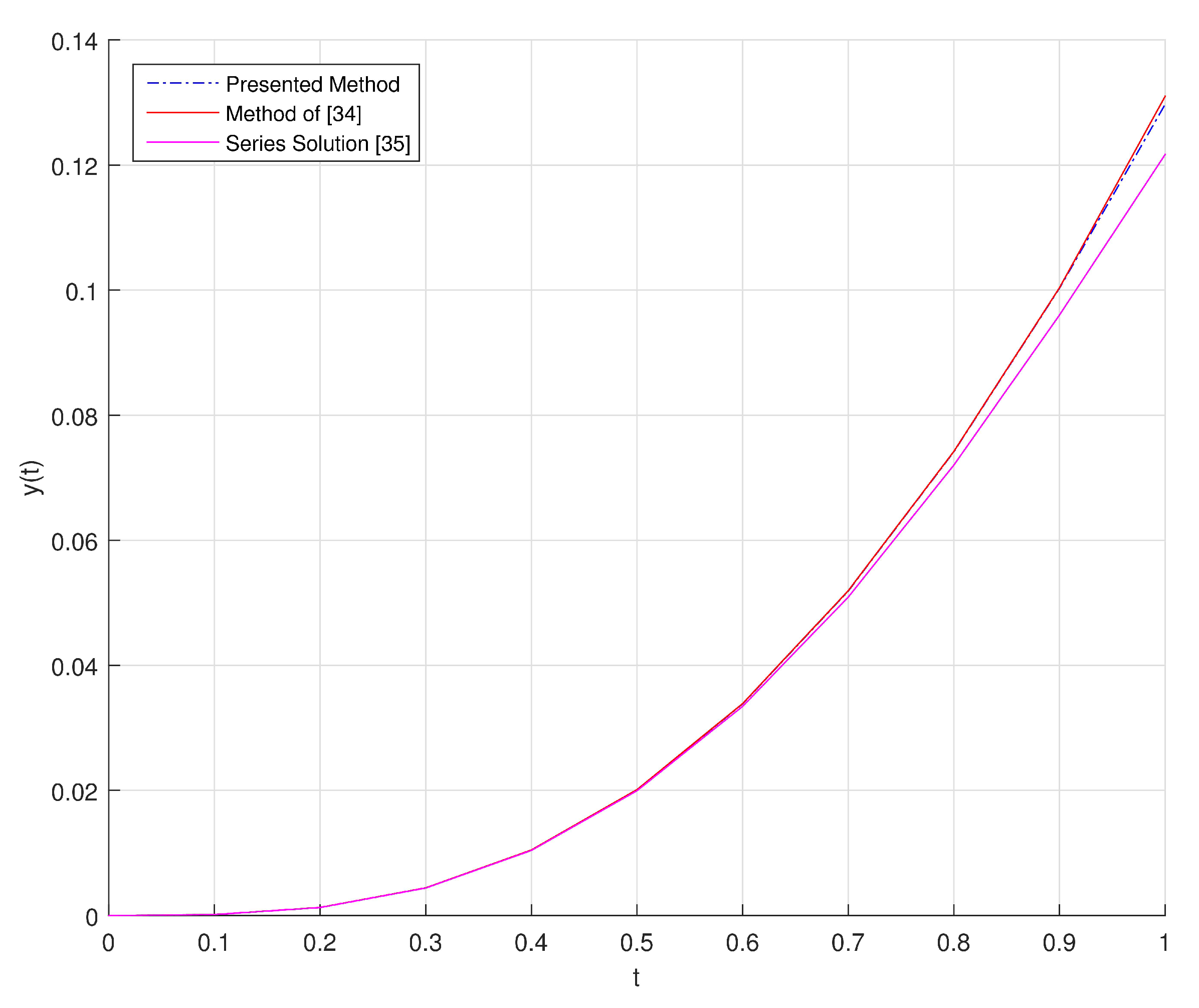
The graphical representation of comparison between series solution and numerical solutions obtained by presented method and the method of [54] in the interval $[0,1]$ is illustrated in Figure 8.

In Figure 9, we show present graphical representation of absolute errors obtained by using proposed method and the method of [54] with $m=10$.

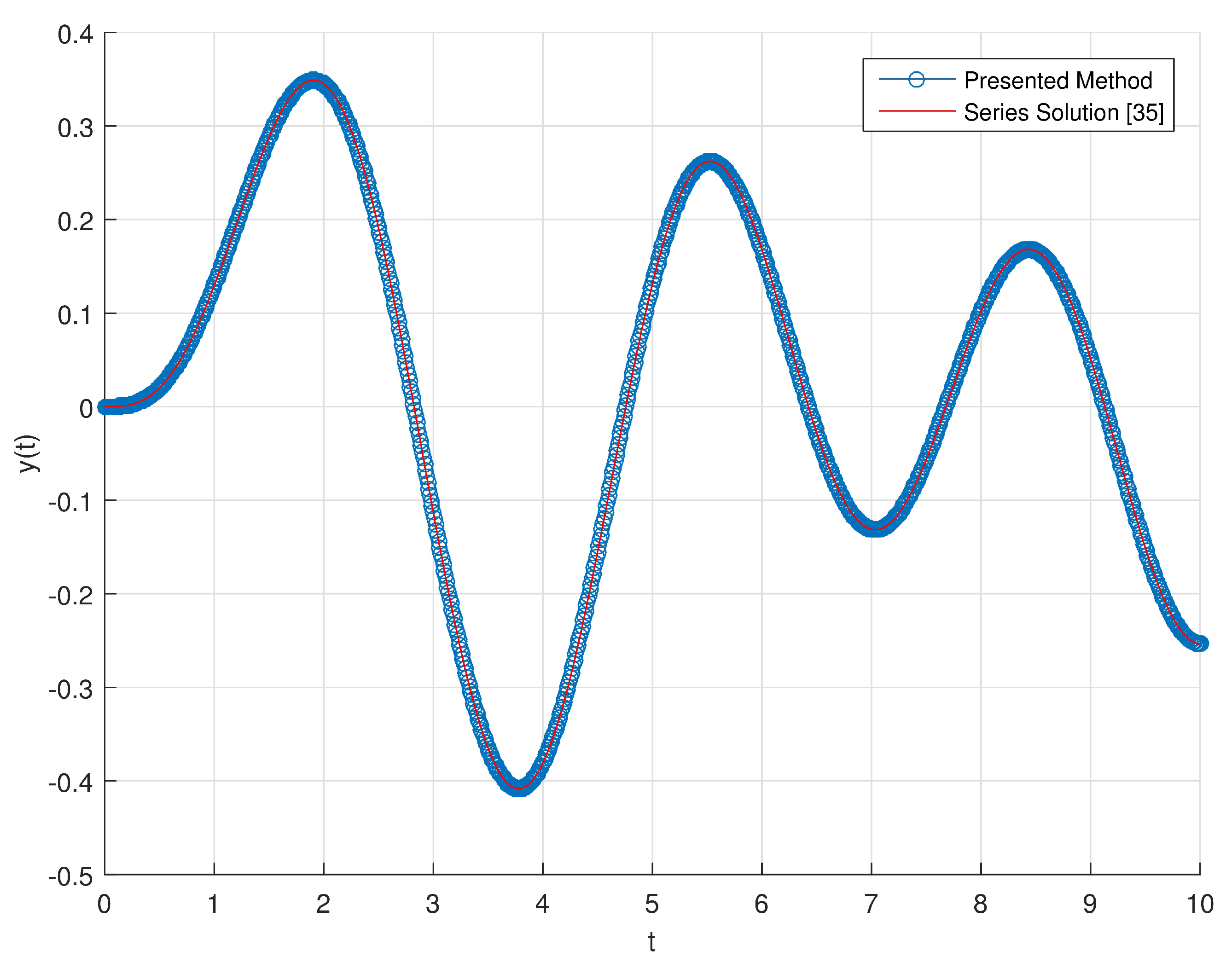
In Figure 10, we show the graphical representation for series solution and the numerical results of presented method for the interval $[0,10]$. The results plotted in Figure 10 are in a very good and satisfactory agreement with the series solution given in [52] and the results of [60].

5.4. Example 4

Motivated by [50], we consider the following form of fractional differential equation,

$$D^{\alpha }y\left(t\right)+y\left(t\right)=\left\{\begin{array}{cc}{\displaystyle \frac{2}{\Gamma (3-\alpha )}{t}^{2-\alpha }+t^2-t,}\hfill & \alpha >1\hfill \\ {\displaystyle \frac{2}{\Gamma (3-\alpha )}{t}^{2-\alpha }-\frac{1}{\Gamma (2-\alpha )}{t}^{1-\alpha }+t^2-t,}\hfill & \alpha \le 1\hfill \end{array}\right.$$

(28)

with initial conditions

$$y\left(0\right)=0,y^{\prime }\left(0\right)=-1$$

whose exact solution is $y\left(t\right)=t^2-t.$

In order to apply the presented method to Equation (28) and compare the results with methods of [54,61,62], we solve this problem with $\alpha =0.3,0.5,0.7,1.25,1.5,1.85,$ and different values for $\delta$ and m. The obtained results are presented as below.

In

Table 5. The absolute errors with m = 3 and $\alpha <1$ for Example 4.

t	$\mathit{\alpha }\mathbf{=}\mathbf{0.3}$	$\mathit{\alpha }\mathbf{=}\mathbf{0.5}$	$\mathit{\alpha }\mathbf{=}\mathbf{0.7}$
0	0	0	0
0.1	4.16 × 10${}^{-17}$	8.33 × 10${}^{-17}$	1.94 × 10${}^{-16}$
0.2	8.33 × 10${}^{-17}$	5.55 × 10${}^{-17}$	2.78 × 10${}^{-16}$
0.3	1.11 × 10${}^{-16}$	2.78 × 10${}^{-17}$	2.50 × 10${}^{-16}$
0.4	1.67 × 10${}^{-16}$	1.39 × 10${}^{-16}$	2.50 × 10${}^{-16}$
0.5	1.67 × 10${}^{-16}$	1.11 × 10${}^{-16}$	1.67 × 10${}^{-16}$
0.6	1.67 × 10${}^{-16}$	5.55 × 10${}^{-17}$	2.78 × 10${}^{-17}$
0.7	1.67 × 10${}^{-16}$	8.33 × 10${}^{-17}$	8.33 × 10${}^{-17}$
0.8	3.05 × 10${}^{-16}$	5.55 × 10${}^{-17}$	1.11 × 10${}^{-16}$
0.9	2.08 × 10${}^{-16}$	1.25 × 10${}^{-16}$	1.39 × 10${}^{-16}$
1.0	1.91 × 10${}^{-16}$	1.26 × 10${}^{-16}$	8.91 × 10${}^{-17}$

, we list the results of obtained absolute errors for $\alpha =0.3,0.5,0.7$ by use of presented method. Also, the results for $\alpha =1.25,1.5,1.85$ are given in

Table 6. The absolute errors with m = 3 and $\alpha >1$ for Example 4.

t	$\mathit{\alpha }\mathbf{=}\mathbf{1.25}$	$\mathit{\alpha }\mathbf{=}\mathbf{1.5}$	$\mathit{\alpha }\mathbf{=}\mathbf{1.85}$
0.0	0	0	0
0.1	1.39 × 10${}^{-17}$	2.78 × 10${}^{-17}$	1.25 × 10${}^{-16}$
0.2	5.55 × 10${}^{-17}$	5.55 × 10${}^{-17}$	1.94 × 10${}^{-16}$
0.3	5.55 × 10${}^{-17}$	5.55 × 10${}^{-17}$	2.22 × 10${}^{-16}$
0.4	5.55 × 10${}^{-17}$	2.78 × 10${}^{-17}$	2.50 × 10${}^{-16}$
0.5	1.11 × 10${}^{-16}$	0	2.22 × 10${}^{-16}$
0.6	1.67 × 10${}^{-16}$	5.55 × 10${}^{-17}$	1.67 × 10${}^{-16}$
0.7	1.94 × 10${}^{-16}$	5.55 × 10${}^{-17}$	5.55 × 10${}^{-17}$
0.8	3.05 × 10${}^{-16}$	1.39 × 10${}^{-16}$	5.55 × 10${}^{-17}$
0.9	1.11 × 10${}^{-16}$	8.33 × 10${}^{-17}$	1.39 × 10${}^{-17}$
1.0	8.21 × 10${}^{-17}$	1.97 × 10${}^{-16}$	1.06 × 10${}^{-16}$

.

In Figure 11a,b, we present the graphical representation of obtained results for numerical and exact solution of the given problem and absolute error for $\alpha =1.5$ in the interval $[0,1]$.

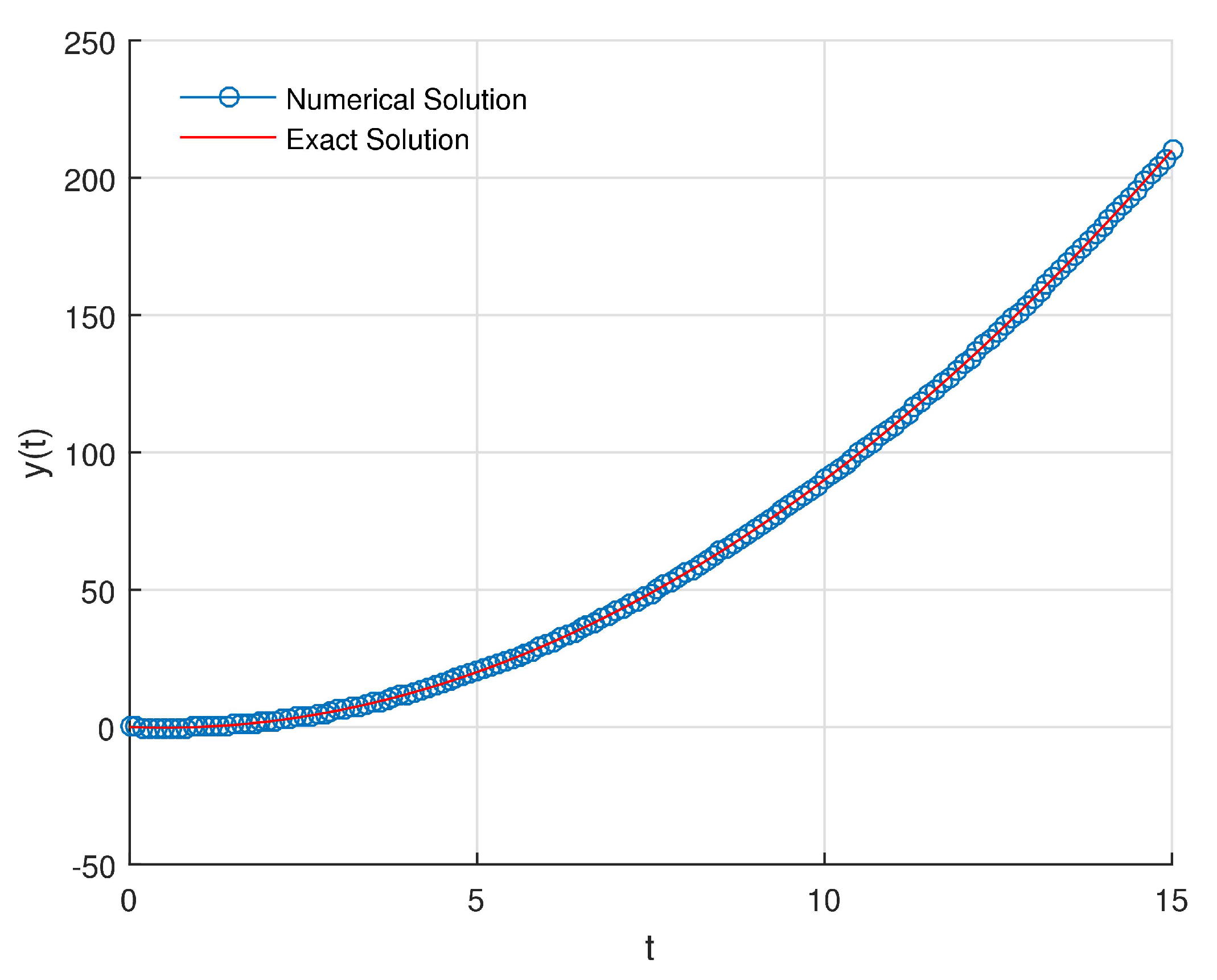
In Figure 12, we plot the graphical representation for behavior of the obtained numerical solution by use of the presented method and the exact solution of the given problem for $\alpha =1.5$ in the interval $[0,15]$.

Table 7. Comparison of absolute errors between proposed method and some other numerical methods in literature at $t=1,5,10,50$ for $\alpha =1.5$.

t	Presented Method	Method of [63]	Method of [50]	Method of [64]
	$\mathit{\delta }=\mathbf{1}/\mathbf{2},\mathit{m}=\mathbf{4}$	$\mathit{n}=\mathbf{20}$	$\mathit{h}=\mathbf{1}/\mathbf{320}$	$\mathit{p}=\mathbf{1},\mathit{T}=\mathbf{1}$
1	7.99361 × 10${}^{-14}$	9.10 × 10${}^{-5}$	3.42 × 10${}^{-3}$	-
5	2.55795 × 10${}^{-13}$	2.42 × 10${}^{-3}$	-	-
10	1.42109 × 10${}^{-13}$	5.50 × 10${}^{-3}$	-	-
50	3.63798 × 10${}^{-12}$	3.74 × 10${}^{-2}$	-	1.2

lists the obtained absolute errors for the given problem (28) at $t=1,5,10,50$ and $\alpha =1.5$ by use of presented method and some other methods in literature [54,61,62]. From this compared results, we can say that the numerical solution obtained by use of proposed method is in better agreement with the exact solution and obtained absolute error is smaller.

In Figure 13, the behaviour of absolute error for $\alpha =1.5$ with $m=4$ and $\delta =1/2,1$ at $t\in [0,50]$ is presented. From this graph, it can be seen that we get better results by taking $\delta =1/2$ for this example and the numerical solution is very close to exact solution for a small number of $m.$

5.5. Example 5

In this example, we consider the following form of linear multi-term fractional differential equation with variable coefficients [65]

$$a{D}^{2}y\left(t\right)+b\left(t\right)D^{{\beta }_1}y\left(t\right)+c\left(t\right)Dy\left(t\right)+e\left(t\right)D^{{\beta }_2}y\left(t\right)+k\left(t\right)y\left(t\right)=f\left(t\right),$$

(29)

with,

$$y\left(0\right)=2,y^{\prime }\left(0\right)=0$$

where $0<{\beta }_2<1,1<{\beta }_1<2$ and

$$f\left(t\right)=-a-\frac{b\left(t\right)}{\Gamma (3-{\beta }_1)}{t}^{2-{\beta }_1}-c\left(t\right)t-\frac{e\left(t\right)}{\Gamma (3-{\beta }_2)}{t}^{2-{\beta }_2}+k\left(t\right)\left(2-\frac{t^2}{2}\right)$$

whose the exact solution is given by $y\left(t\right)=2-\frac{t^2}{2}.$

We give the numerical solution for the given problem by proposed method for $a=1,b\left(t\right)=\sqrt{t},c\left(t\right)=t^{\frac{1}{3}},e\left(t\right)=t^{\frac{1}{4}},k\left(t\right)=t^{\frac{1}{5}},{\beta }_2=0.333,{\beta }_1=1.234$ with $\delta =1$.

In

Table 8. Maximum errors of Example 5 for $R=1$ with $m=3,4,5,6,10,20,40$.

m	Present Method	Method Given in [66]	Method Given in [65]
3	4.44089 × 10${}^{-16}$	4.4409 × 10${}^{-16}$	-
4	6.66134 × 10${}^{-16}$	1.4633 × 10${}^{-13}$	-
5	4.44089 × 10${}^{-16}$	3.2743 × 10${}^{-12}$	6.88384 × 10${}^{-5}$
6	4.44089 × 10${}^{-16}$	1.0725 × 10${}^{-13}$	-
10	2.22045 × 10${}^{-15}$	-	3.00351 × 10${}^{-6}$
20	3.47278 × 10${}^{-13}$	-	1.67837 × 10${}^{-7}$
40	1.46549 × 10${}^{-13}$	-	1.02241 × 10${}^{-8}$

, we give the results for maximum errors obtained by use of proposed method and comparison with the results of [65,66]. From this compared results, we can see that the numerical solution obtained by use of proposed method is closer to the exact solution.

Figure 14 presents the graphical representation for behaviour of numerical and exact solutions with $m=6$. From this representation, we can see that the numerical solution is in a very good agreement with exact solution.

5.6. Example 6

For the last example, let us consider the below fractional differential equation [63]

$$\begin{array}{cc}\hfill y^{\prime }\left(t\right)+D^{1/2}y\left(t\right)-2y\left(t\right)& =0,t\in (0,R],\hfill \\ \hfill y\left(0\right)& =1\hfill \end{array}$$

(30)

which arises, for example, in the study of generalized Basset force occuring when a spherical object sinks in a (relatively dense) incompressible viscous fluid; see [43,67]. By use of Laplace transformation of Caputo derivatives, we get the analytical solution as following

$$y\left(t\right)=\frac{2}{3\sqrt{t}}{E}_{1/2,1/2}\left(\sqrt{t}\right)-\frac{1}{6\sqrt{t}}{E}_{1/2,1/2}(-2\sqrt{t})-\frac{1}{2\sqrt{\pi t}},$$

where the Mittag–Leffler function $E_{\lambda ,\mu }\left(t\right)$ with parameters $\lambda ,\mu >0$ is given as

$$E_{\lambda ,\mu }\left(t\right)=\sum _{k=0}^{\infty }\frac{t^k}{\Gamma (\lambda k+\mu )}.$$

This Mittag–Leffler function and its variations are very significant in fractional calculus and fractional differential equations [68].

In order to solve given problem by use of proposed method and compare the results, we take $t\in (0,5]$ and use different values of $\delta$ and m.

Table 9. The resulting values for Example 6, with $R=5$ in some values of t.

t	Exact	Proposed Method	Method Given in [63]	Proposed Method	Method Given in [63]	Proposed Method	Method Given in [63]	Proposed Method	Method Given in [63]
		$\mathit{m}=\mathbf{5}$	$\mathit{m}=\mathbf{5}$	$\mathit{m}=\mathbf{10}$	$\mathit{m}=\mathbf{10}$	$\mathit{m}=\mathbf{15}$	$\mathit{m}=\mathbf{15}$	$\mathit{m}=\mathbf{20}$	$\mathit{m}=\mathbf{20}$
1	3.42445	3.42415	2.714336	3.425121	3.426525	3.42376044	3.42496	3.424563	3.424807
2	9.69088	9.670891	8.922571	9.692732	9.696794	9.68896761	9.692754	9.691185	9.691706
3	26.6414	26.60757	24.59981	26.64646	26.65929	26.6362145	26.64683	26.64225	26.64381
4	72.6729	72.53849	65.78029	72.68665	72.72038	72.6587861	72.68787	72.6752	72.67936
5	197.77	197.5757	180.1481	197.8077	197.8994	197.731934	197.8112	197.7766	197.7879

lists the exact and obtained numerical solutions by use of presented method and method of [63] for the given problem for $m=5,10,15,20$. Comparison of this results shows that, even for small values of m, the numerical solution obtained by use of presented method is in a better agreement with exact solution.

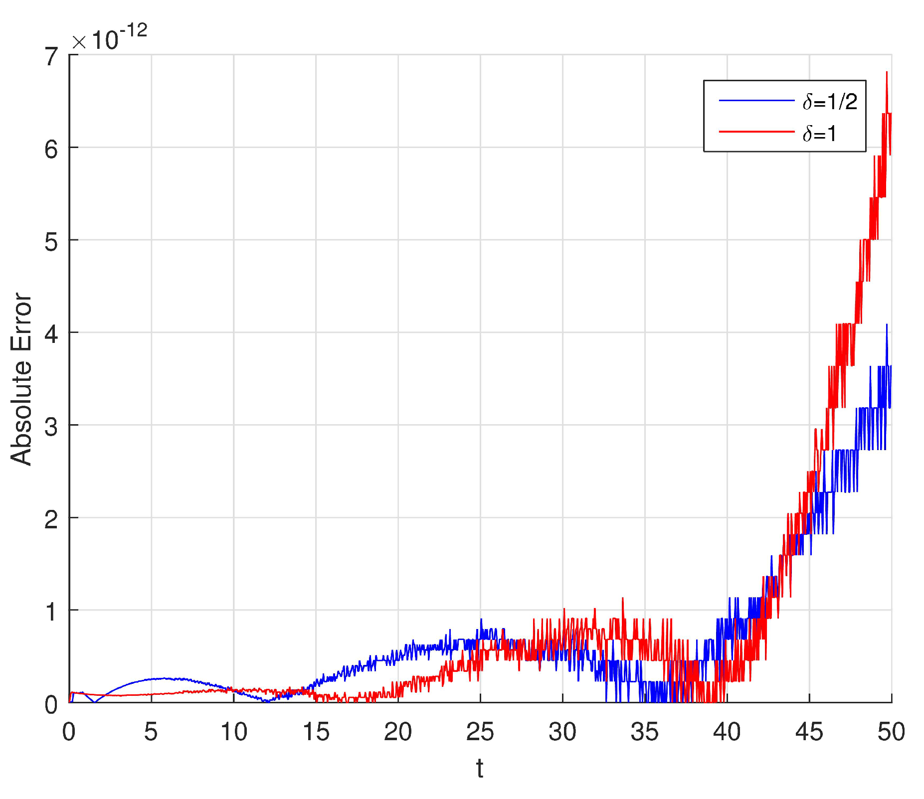
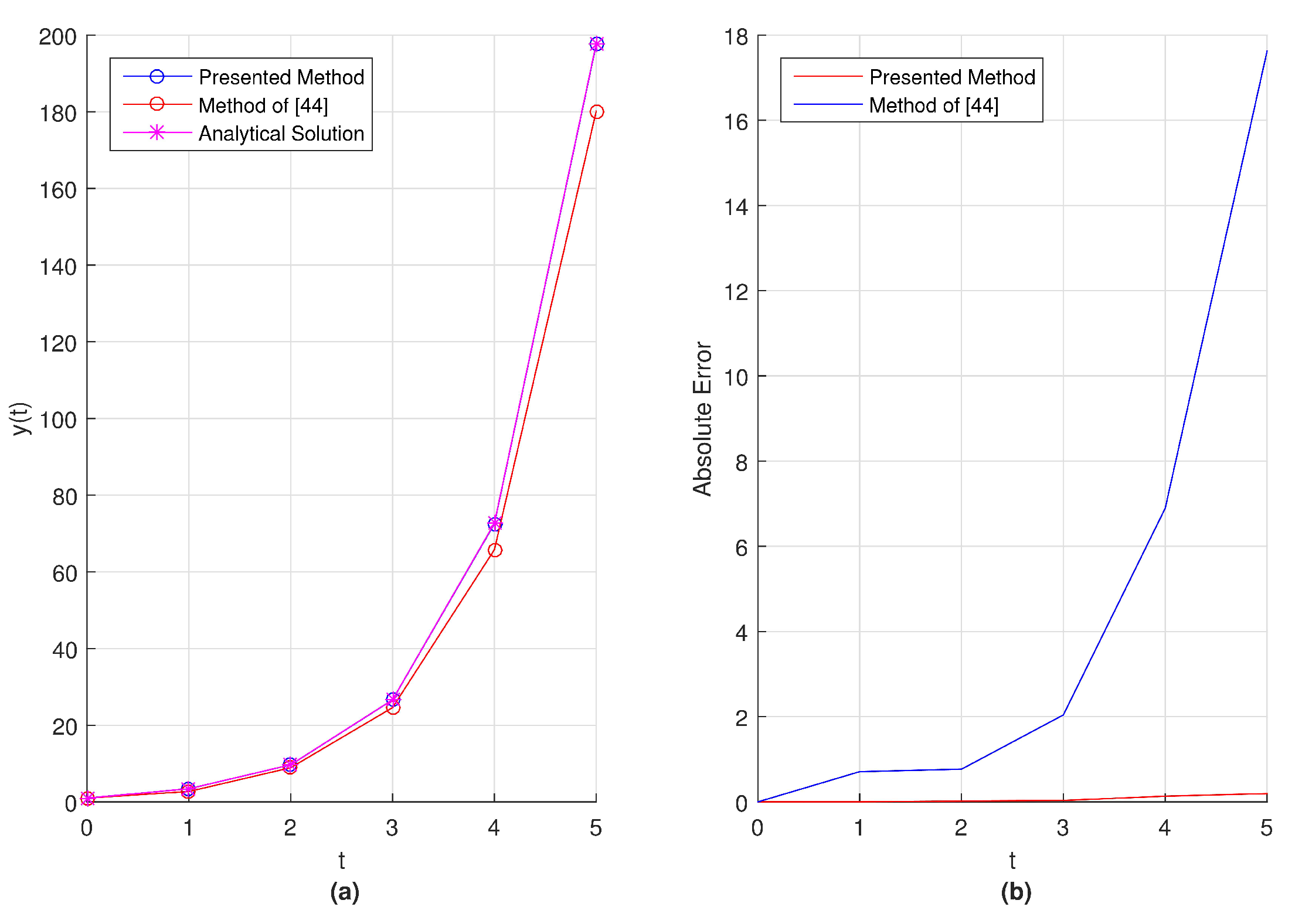
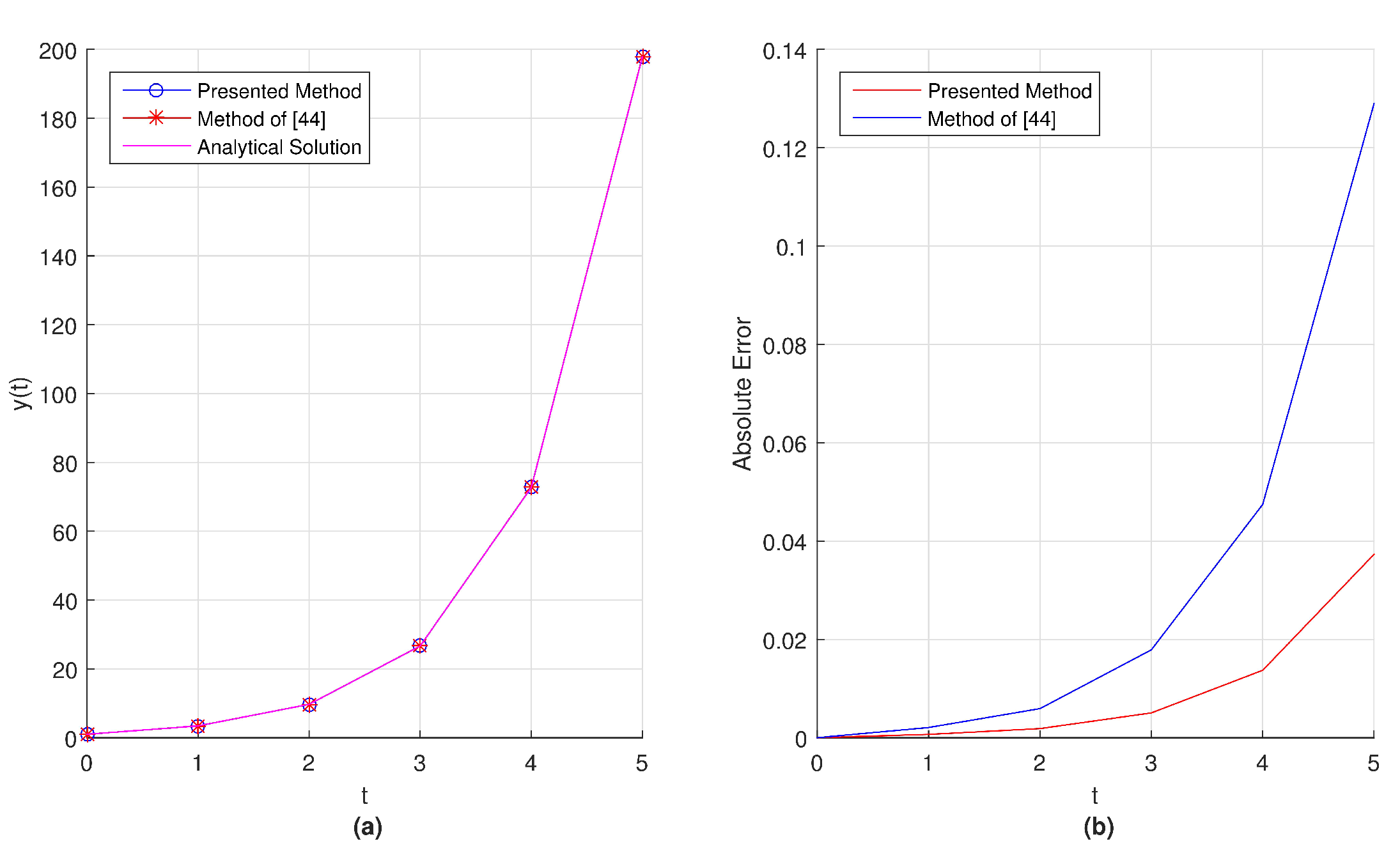
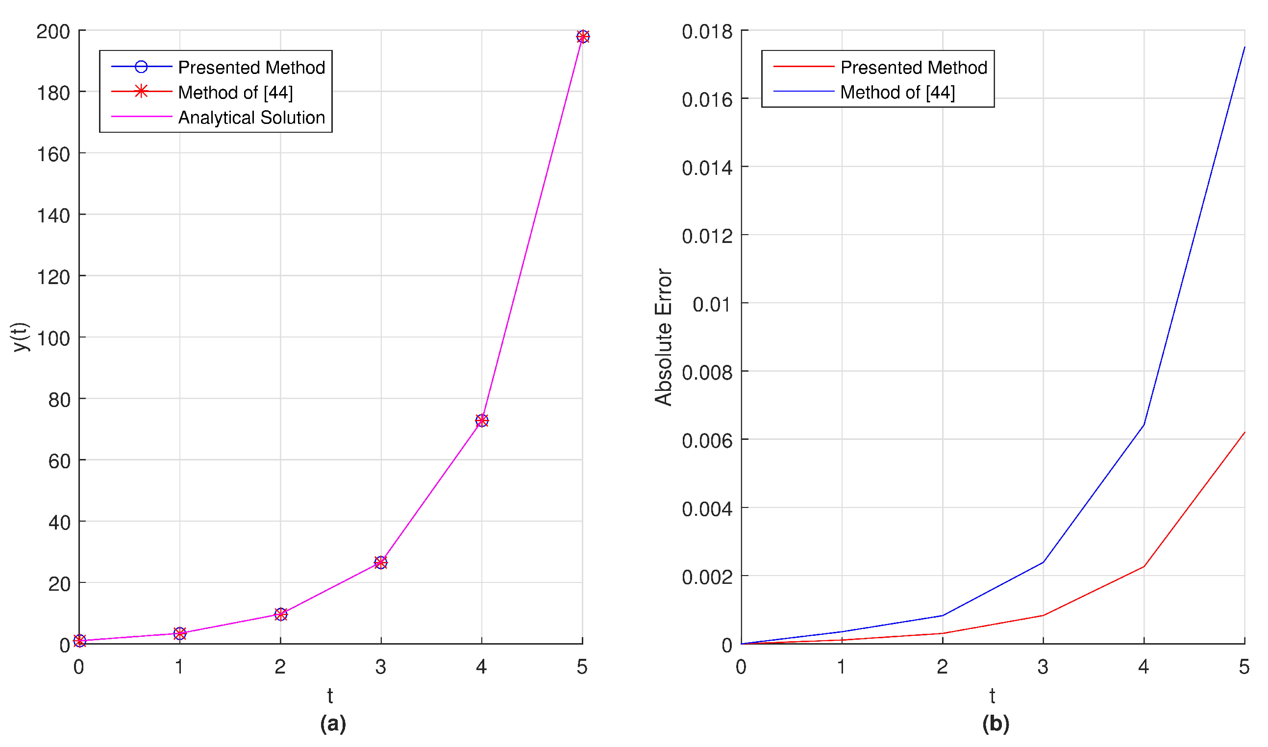
In Figure 15a, Figure 16a and Figure 17a, we present the graphical representation of comparison between exact solution and the numerical solutions obtained by using proposed method and the method of [63] with taking $m=5,10,20$ respectively. Also in Figure 15b, Figure 16b and Figure 17b we show the behaviour of absolute errors obtained by proposed method and the method of [63] in the interval $[0,1]$ with $m=5,10,20$.

From these graphical results represented in Figure 15, Figure 16 and Figure 17, we can conclude that the absolute error obtained by our method is remaining smaller when compared the absolute error of method given in Reference [63].

6. Conclusions

In this work, an operational matrix based on the fractional Taylor vector is used to numerically solve the multi-term fractional differential equations by reducing them to a set of linear algebraic equations, which simplifies the problem. From comparison of the obtained results with exact solutions and also with results of other methods in the literature, we conclude that the proposed method provides the solution with high accuracy. The findings also show that, even for the small number of steps, we can get satisfactory results by using presented method. All computational results are obtained by using MATLAB.