Reinterpretation of Multi-Stage Methods for Stiff Systems: A Comprehensive Review on Current Perspectives and Recommendations

Abstract

In this paper, we compare a multi-step method and a multi-stage method for stiff initial value problems. Traditionally, the multi-step method has been preferred than the multi-stage for a stiff problem, to avoid an enormous amount of computational costs required to solve a massive linear system provided by the linearization of a highly stiff system. We investigate the possibility of usage of multi-stage methods for stiff systems by discussing the difference between the two methods in several numerical experiments. Moreover, the advantages of multi-stage methods are heuristically presented even for nonlinear stiff systems through several numerical tests.

1. Introduction

Most time-dependent differential equations are usually solved by multi-stage (one-step) method or multi-step method [1,2,3]. In general, there seems to be no significant difference in the structure between them when the multi-stage method is applied to get an initial guess for the multi-step method [4]. Nonetheless, a comparison of both methods has attracted quite a lot of interest from the viewpoints of convergence, stability, practical computations, numerical efficiency, etc. [5,6,7,8,9,10,11]. Comparisons in this regard do not take into account the impact of advances in computer science and technologies such as artificial intelligence (AI) or parallel computation, etc. Considering the impact, a new perspective to compare the potentials of both methods should be investigated as well as existing comparative studies. First of all, it is well known that the highest order of an A-stable multi-step method is two, so lots of research [12,13,14,15,16,17,18,19,20,21,22,23,24] developing higher order methods have focused on either multi-step methods satisfying some less restrictive stability condition or multi-stage methods which combine A-stability with high-order accuracy [2,25,26,27,28,29]. In addition, multi-stage methods such as Runge–Kutta (RK) type methods do not require any additional memory for function values at previous steps since it does not use any previously computed values [30,31,32]. On the other hand, multi-step methods require additional memory in the sense that they use previously computed function values and have insufficient function values for initial data. Multi-stage methods are comparable with multi-step methods for nonlinear stiff problems and have no restriction to express initial data contrast to the other. There seems not to be such a clear a priori distinction between multi-stage and multi-step methods.

Another interesting point of view to find more efficient methods is quite susceptible to stiffness and nonlinearity of the given problem. For nonlinear stiff problems, a multi-step method is needed to evaluate function values only once at each iteration in a nonlinear solver, whereas multi-stage methods require several function evaluations at each iteration. This disadvantage of the multi-stage method can be ignored by the authors’ recent research [33]. The authors showed numerically that one stage of the multi-stage method is equivalent to one step of the multi-step method for simple ordinary differential equation (ODE) systems. However, the multi-step methods such as the backward differentiation formula (BDF) are usually recommended to apply nonlinear stiff problems because the process of solving the nonlinear system of equation is also expensive computationally. In the process of solving nonlinear stiff problems by a multi-stage method, it generally generates a system $M_d\otimes M_s$, where d and s represent the dimension of the given problem and the number of stages used in the multi-stage method, respectively. Here, the notation $M_k$ represents a matrix with the size $k\times k$ and the notation ⊗ denotes a Kronecker product. On the other hand, a multi-step method needs to solve only a system of size $d\times d$.

The purpose of this paper is to investigate and compare the properties of the multi-stage and the multi-step methods for d-dimensional stiff problems described by

$$\begin{array}{c}\hfill \frac{dy}{dt}=f(t,y)\in {\mathbb{R}}^d.\end{array}$$

(1)

Most nonlinear stiff problems are solved by multi-step methods rather than multi-stage methods since the multi-stage methods usually transform nonlinear stiff problems into bigger nonlinear systems, as mentioned in the previous paragraph. To solve such nonlinear systems efficiently, one has to consider both nonlinear and linear solvers. The nonlinear systems are usually solved by using an iteration technique such as Newton-like iterations, which incur considerable computation costs. There are various Newton-like iterations. Among them, a simplified Newton iteration is developed in connection with the development of computer process capacity [34,35,36,37]. Different nonlinear system solvers generate linear systems correspondingly. It means that the nonlinear system solver should be well-selected to adapt efficient linear solvers such as the eigenvalue decomposition method. Note that efficient linear solvers have also been well-studied [1,2,38,39]. An eigenvalue decomposition combined with simplified Newton iteration can apply to a multi-stage method. The resulting multi-stage method generates the same matrix, regardless of integration or iteration, as an object of decomposition for solving a linear system induced by the simplified Newton iteration. It allows for decomposing the matrix only once throughout the whole process. As a result, applying this combination to multi-stage methods highlights the advantage of multi-stage methods by reducing computational costs to the level of the costs required from multi-step methods without any loss of the original advantages of multi-stage methods, which is the main contention of this paper.

The remaining parts of this paper are as follows. We briefly describe the multi-step and multi-stage methods and simplified Newton iteration in Section 2. To support theoretical analysis, we present preliminary numerical results in Section 3. Finally, in Section 4, all results are summarized and further possibilities are discussed.

2. Preliminary

2.1. Methods

In this subsection, we briefly describe ODE solvers classified by mathematical theory. Numerical methods for ODEs fall naturally into two categories: one is ‘multi-stage method’ using one starting value at each step and the other is ‘multi-step method’ or ‘multi-value method’ based on several values of the solution. We deal with the theories of two methods in terms of convergence and stability. The multi-step method has a critically bad stability property with a higher convergence rate that can not actually be used. Due to these reasons, the third-order RK method (RK3) and the third-order BDF (BDF3) are considered as examples of multi-stage methods and multi-step methods. Note that the higher order multi-step method is also available, but it has very low practical use.

The general form of the multi-step methods [1,3,7,26,38,40,41] is described by

$$\begin{array}{c}\hfill y_{n+1}=\sum _{j=0}^s{a}_j{y}_{n-j}+h\sum _{j=-1}^s{b}_{j}f(t_{n-j},y_{n-j}),n\ge s.\end{array}$$

(2)

Here, the coefficients $a_0,\dots ,a_s,b_{-1},b_0,\dots ,b_s$ are constants. If method (2) use $s+1$ previous solution values with either $a_s\ne 0$ or $b_s\ne 0$, the method is called an $s+1$ step method. A BDF method is the most efficient linear multi-step methods among several multi-step methods [40]. It is composed of the coefficients $b_{p-1}=\cdots =b_0=0$ and the others chosen such that the method with the convergence order of s convergence order s. Thus, the s-step BDF has s-th convergence order. The BDF3 is given by

$$\begin{array}{c}\hfill y_{n+3}-\frac{18}{11}{y}_{n+2}+\frac{9}{11}{y}_{n+1}-\frac{2}{11}{y}_n=\frac{6}{11}hf(t_{n+3},y_{n+3}).\end{array}$$

(3)

Since implicit A-stable linear multi-step methods have convergence order of at most 2, second-order BDF can be A-stable, but the method can not be A-stable with order more than 3. The stability of BDF3 is almost A-stable [38].

An explicit RK method has been developed by Runge, Heun, and Kutta based on a Euler method [3,40]. Later, an implicit RK was developed for stiff problems based on several quadrature rules. RK methods have the following form:

$$\begin{array}{c}\hfill \begin{array}{cc}\hfill & y_{n+1}=y_n+h\sum _{i=1}^s{b}_i{k}_i,\hfill \\ \hfill & k_i=f(t_n+c_{i}h,y_n+h\sum _{j=1}^s{a}_{ij}{k}_j),i=1,\dots ,s,\hfill \end{array}\end{array}$$

(4)

or an equivalent form of Butcher tableau

$$\begin{array}{cc}c& A\\ & b\end{array}.$$

One can specify a particular RK method by providing the number of stage s and all elements of the Butcher tableau, $a_{ij}$ ($1\le i,j\le s$), $b_i$ and $c_i$ ($i=1,\dots ,s$). There is a popular implicit RK method for solving the stiff problem, which is called a collocation method. The collocation method is changed depending on the choice of the collocation points. For more details on the collocation method, one can refer to [3,38]. If we select uniform collocation points defined by $c_i=i/3$ ($1\le i\le 3$), we can obtain a third-order collocation method with having the following butcher table:

$$\begin{array}{cccc}\frac{1}{3}& \frac{23}{36}& -\frac{4}{9}& \frac{5}{36}\\ \frac{2}{3}& \frac{7}{9}& -\frac{2}{9}& \frac{1}{9}\\ 1& \frac{3}{4}& 0& \frac{1}{4}\\ & \frac{3}{4}& 0& \frac{1}{4}\end{array}.$$

(5)

Note that the order of the stage and convergence for the method (5) are both three as shown in the convergence analysis in [3,38]. Furthermore, the stability of (5) demonstrated through Dahlquist’s problem is almost L-stable.

2.2. Simplified Newton Iteration and Eigenvalue Decomposition Method

To explicate a simplified Newton iteration proposed by Liniger and Willoughby [10], we consider the following nonlinear system obtained by RK-type methods,

$$\begin{array}{c}\hfill z_i=h\sum _{j=1}^s{a}_{ij}f(x_0+c_{j}h,y_0+z_j),i=1,\dots ,s.\end{array}$$

(6)

Equation (6) is equivalent to a system of equations described by

$$Z=h(A\otimes I_d))F\left(Z\right),$$

(7)

where

$$\begin{array}{cc}\hfill & Z={[z_1,\dots ,z_s]}^T,\hfill \\ \hfill & A={\left(a_{ij}\right)}_{i,j=1}^s,\hfill \\ \hfill & F\left(Z\right)={[f(x_0+c_{1}h,y_0+z_1),\dots ,f(x_0+c_{s}h,y_0+z_s)]}^T,\hfill \end{array}$$

and $I_d$ is d-dimensional identity matrix. By applying Newton iteration to the nonlinear system of Equation (7), we can get a linear system of the form

$$\begin{array}{c}\hfill \begin{array}{cc}\hfill \left(I_{sd}-h(A\otimes I_d)\mathcal{J}\right)\Delta Z^k& =-Z^k+h(A\otimes I_d)F\left(Z^k\right),\hfill \\ \hfill Z^{k+1}& =Z^k+\Delta Z^k,\hfill \end{array}\end{array}$$

(8)

where $\mathcal{J}$ is a block diagonal matrix that consists of Jacobians $\frac{\partial f}{\partial y}(t_n+c_{i}h,y_n+z_i)$, $i=1,\dots ,s$, $Z^k={(z_1^k,\dots ,z_s^k)}^T$ is the k-th iterated solution, $\Delta Z^k={(\Delta z_1^k,\dots \Delta z_s^k)}^T$ is the increment, and $F\left(Z^k\right)$ denotes for

$$\begin{array}{c}\hfill F\left(Z^k\right)={(f(x_0+c_{1}h,y_0+z_1^k),\dots ,f(x_0+c_{s}h,y_0+z_s^k))}^T.\end{array}$$

Usually, one Newton iteration needs several calculations of the Jacobian which requires lots of computational costs. To reduce such costs, all Jacobians $\frac{\partial f}{\partial y}(t_n+c_{i}h,y_n+z_i)$ are replaced by $\frac{\partial f}{\partial y}(t_n,y_n)$. This process is called ’simplified Newton iteration’. The simplified Newton iteration for (7) leads (9) to the formula

$$\begin{array}{c}\hfill \begin{array}{cc}\hfill (I_{sd}-hA\otimes J)\Delta Z^k& =-Z^k+h(A\otimes I_d)F\left(Z^k\right),\hfill \\ \hfill Z^{k+1}& =Z^k+\Delta Z^k,\hfill \end{array}\end{array}$$

(9)

where $J:=\frac{\partial f}{\partial y}(t_n,y_n)$. Each iteration requires s times evaluation of f and the calculations of a $d·s$-dimensional linear system.

Note that, by using the simplified Newton iteration, the matrix $(I-hA\otimes J)$ is the same for all iterations, so the decomposition method for solving the resulting linear system can be needed only once. For the linear system, we consider an eigenvalue decomposition technique in that it decomposes the given $d·s$ dimensional linear system into several s-dimensional linear systems. In the view of computational efficiency, it is more efficient to calculate several small size systems even if it is a complex system, rather than to calculate one big size system. Note that only a simplified Newton iteration (9) enables usage of eigenvalue decompositions that cannot be applicable to traditional Newton iteration (8). The eigenvalue decomposition method for (9) is proposed independently by Butcher [31] and Bickart [30]. The main ideas of the method are eigenvalue decomposition of the matrix $A^{-1}=T\mathsf{\Lambda }{T}^{-1}$ and linear transformation of the vector $Z^k$. By transforming $W^k=(T^{-1}\otimes I)Z^k$, the iteration (9) becomes equivalent to

$$\begin{array}{c}\hfill \begin{array}{cc}\hfill (h^{-1}\mathsf{\Lambda }\otimes I_d-I_3\otimes J)\Delta W^k& =-h^{-1}(\mathsf{\Lambda }\otimes I_d)W^k+(T^{-1}\otimes I_d)F\left((T\otimes I)W^k\right),\hfill \\ \hfill W^{k+1}& =W^k+\Delta W^k.\hfill \end{array}\end{array}$$

(10)

In a general case of the three-stage implicit RK method such as (5), the inverse matrix of A has an eigenvalue decomposition as follows:

$$A^{-1}=T\mathsf{\Lambda }{T}^{-1}=\left[\begin{array}{ccc}{u}_0,& u_1,& -v_1\end{array}\right]\left[\begin{array}{ccc}\widehat{\gamma }& 0& 0\\ 0& \widehat{\alpha }& -\widehat{\beta }\\ 0& \widehat{\beta }& \widehat{\alpha }\end{array}\right]{\left[\begin{array}{ccc}{u}_0,& u_1,& -v_1\end{array}\right]}^{-1},$$

(11)

where $\widehat{\gamma }$ is one real real eigenvalue, $\widehat{\alpha }\pm i\widehat{\beta }$ are one complex eigenvalue pair and $u_0$, and $u_1\pm v_1$ are eigenvectors corresponding to $\widehat{\gamma }$, $\widehat{\alpha }\pm i\widehat{\beta }$, respectively. Therefore, the matrix in (10) can be rewritten as

$$\left[\begin{array}{ccc}\gamma I_d-J& 0& 0\\ 0& \alpha I_d-J& -\beta I_d\\ 0& \beta I_d& \alpha I_d-J\end{array}\right]$$

(12)

with $\gamma =\widehat{\gamma }/h,\alpha =\widehat{\alpha }/h,\beta =\widehat{\beta }/h$ so that (10) can be split into two linear systems of dimension d and $2d$, respectively. Moreover, the $2d$-dimensional real valued subsystem can be transformed to the following d-dimensional complex valued system

$$\begin{array}{c}\hfill \left((\alpha +i\beta )I-J\right)(u+iv)=a+ib.\end{array}$$

(13)

In terms of computational cost, the number of multiplication to solve (13) is approximately $4d^3/3$, since the complex multiplication consists of four real multiplications. Then, the total multiplication number for (12) is about $5d^3/3$, while the number of multiplications for decomposing the untransformed matrix $(I-hA\otimes J)$ in (9) is about ${\left(3d\right)}^3/3$. Thus, we can reduce the number of multiplications to about $80\%$ by calculating (12) instead of directly calculating the inverse of the matrix of $(I-hA\otimes J)$ in (10). Finally, to solve the transformations $Z^k=(T\otimes I)W^k$, it additionally requires a multiplication of $\mathcal{O}\left(n\right)$. This difference becomes more apparent as the size of the matrix (or the numbers of stage) increases.

3. Numerical Comparison

In this section, we experiment five commonly used physical examples for comparison of both methods. In Section 3.1, Section 3.2 and Section 3.3, the BDF3 method (3) and RK3 (4) with its butcher table (5) are used as an example of multi-step and multi-stage methods, respectively. The initial guess for BDF3 is taken by exact values. Both methods use the traditional Newton iteration for solving nonlinear systems. In Section 3.3, especially, we measure CPU-time to compare the two methods in terms of accuracy and efficiency and simplified Newton iteration is used for a nonlinear solver. In Section 3.4 and Section 3.5, we use RADAU5 and ODE15s representing a multi-stage and a multi-step method, respectively, which numerical codes are well optimized and open-source. Note that RADAU5, one of multi-stage methods, has convergence order 5 and stage order 3 [38] and ODE15s, one of multi-step methods, included MATLAB library, has variable orders from 1 to 5 [42]. Remarkably, RADAU5 has applied the eigenvalue decomposition and simplified Newton iteration. All numerical simulations are executed with the software MATLAB 2010b (Mathworks, Natick, MA, USA) under OS WINDOWS 7 (Microsoft, Redmond, WA, USA). Note that most numerical results in this section are repeatable even if different computational resources are used.

3.1. Simple Linear ODE

As the first example, we consider the Prothero–Robinson problem [29],

$$\begin{array}{c}\hfill f(t,y\left(t\right))=\nu (y\left(t\right)-g\left(t\right))+g^{\prime }\left(t\right),t\in (0,10],y\left(0\right)=g\left(0\right),\end{array}$$

(14)

which presents a stiffness by varying the parameter $\nu$. The analytic solution of problem is given by $y\left(t\right)=g\left(t\right)$. To compare the error behaviors of the two methods, we set up the parameter $\nu =-1.0\times {10}^6$ so that the given problem can be highly stiff. Here, the exact solution of this problem is set by $g\left(t\right)=sin\left(t\right)$. In Figure 1, we display absolute errors $|y\left(t_i\right)-y_i|$ at each integration step in a log scale obtained by the two methods with different time step sizes $h=2^{-k}$, (a) $k=1$, (b) $k=2$ and (c) $k=3$. One can see that the error of BDF3 (Red) has magnitude (a) $1.0\times {10}^{-7}$, (b) $1.0\times {10}^{-8}$, and (c) $1.0\times {10}^{-9}$. The error of RK3 (Blue) has magnitude (a) $1.0\times {10}^{-9}$, (b) $1.0\times {10}^{-10}$, and (c) $1.0\times {10}^{-11}$. All three graphs in Figure 1 show that RK3 has better accuracy than BDF3. Additionally, to demonstrate the meaning of the stage of multi-stage methods and the step of multi-step methods, we set up a time step size of the multi-step method, BDF3, as $\tilde{h}=h/3$. The result of BDF3 with $\tilde{h}=h/3$ is labeled as BDF3c hereafter. It can be seen that the result from BDF3c (Black) has the same accuracy, compared with RK3. Therefore, it is sufficient to see a comparison of RK3 and BDF3c for further comparison.

3.2. Nonlinear Stiff ODE System: Multi-Mode Problem

As the second example, we consider a nonlinear ODE system based on the Prothero–Robinson problem. The system is given by

$$\begin{array}{cc}\hfill & f(t,Y\left(t\right))=-\mathsf{\Lambda }{(Y\left(t\right)-g\left(t\right)·{\mathbf{1}}_N)}^{\delta }+g^{\prime }\left(t\right)·{\mathbf{1}}_N,t\in (0,10],\hfill \\ \hfill & Y\left(0\right)={(0,\dots ,0)}^T\in {\mathbb{R}}^N,\hfill \end{array}$$

(15)

where $g\left(t\right)=sin\left(t\right)$, ${\mathbf{1}}_N={(1,\dots ,1)}^T\in {\mathbb{R}}^N$ and N is the number of dimension. The exact solution is $Y\left(t\right)=sin\left(t\right)·{\mathbf{1}}_N$. The stiffness of (15) can be controlled by the eigenvalues of the matrix $\mathsf{\Lambda }$, where $\mathsf{\Lambda }$ is diagonal matrix that has elements ${\lambda }_i=1.0e+k_i$$(i=1,\dots ,N)$, $k_i$ is random integer between 0 and 6. In addition, a linearity of the problem depends on the parameter $\delta$. In this experiment, $\delta =1$ and $\delta =5$ are taken for linear and nonlinear cases, respectively. The parameter set $(N,h)=(100,2^{-3})$ is used for both linear and nonlinear cases.

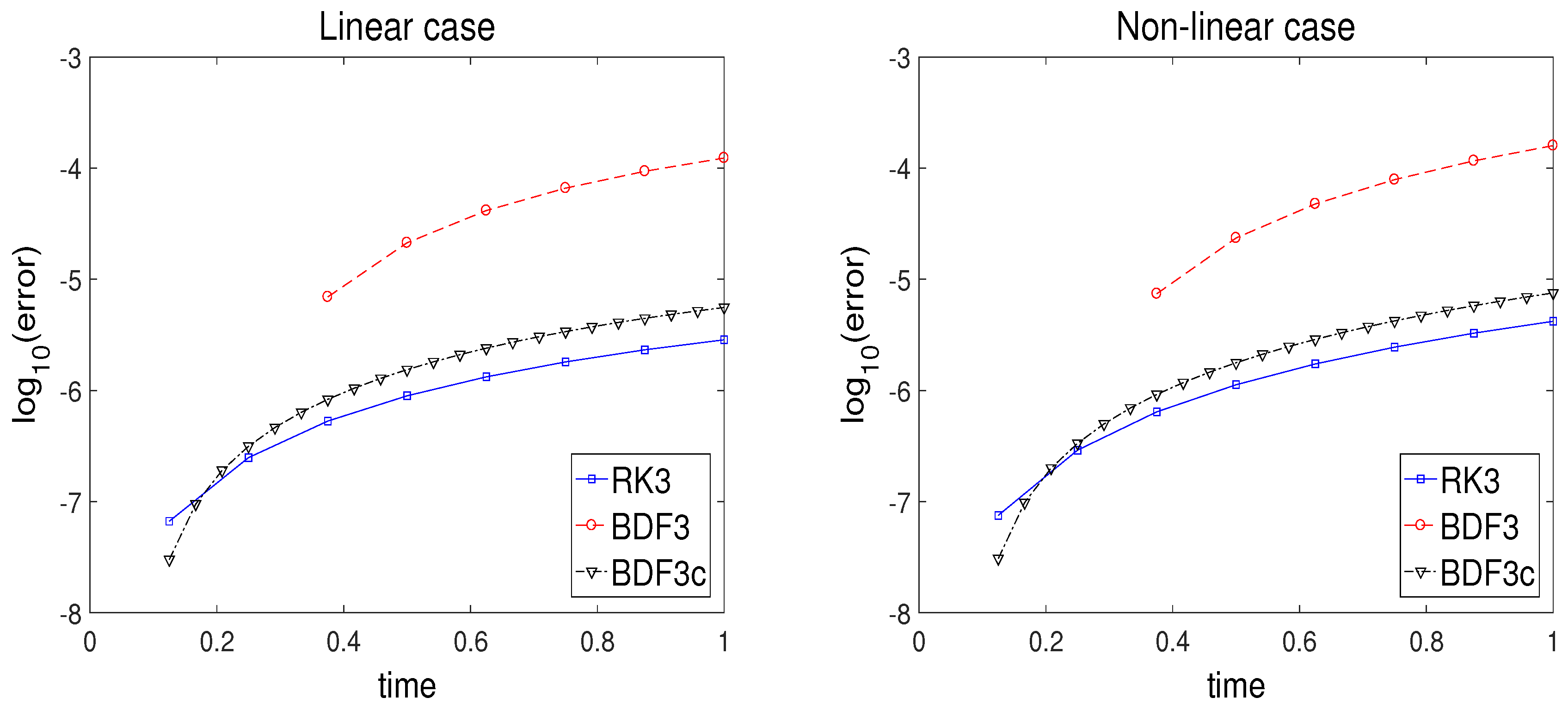
As similar to the previous subsection, the error behaviors of two methods for both linear and nonlinear cases are observed over time, and the results are plotted in Figure 2. The error is measured as $L_{\infty }$-norm at each integration step, $\left|\right|Y\left(t_i\right)-Y_i{\left|\right|}_{\infty }$. For the nonlinear case, a traditional Newton iteration is used for a linearization. As mentioned in the previous subsection, BDF3c uses a smaller time step size $\tilde{h}=h/3$ and is compared with RK3 with time step h. Just in case, we mention that BDF3 with time step h is not appropriate to compare RK3 with the same time step size because of the meaning of the stage, explained in the previous subsection. In the linear case, $\delta =1$, RK3, and BDF3c have similar error behaviors as $1.0\times {10}^{-5.544}$ and $1.0\times {10}^{-5.253}$ at the final time point, respectively. In the nonlinear case, $\delta =5$, RK3, and BDF3 also have similar error behaviors as $1.0\times {10}^{-5.378}$ and $1.0\times {10}^{-5.123}$ at the final time, respectively.

3.3. Linear PDE—Heat Equation

We consider a linear partial differential equation (PDE), the heat equation generally described by

$$\begin{array}{c}\hfill u_t=u_{xx},(t,x)\in [0,1]\times [0,1]\end{array}$$

(16)

with initial value $u(0,x)=sin\left(\pi x\right)+\frac{1}{2}sin\left(3\pi x\right)$ and boundary conditions $u(t,0)=u(t,1)=0$. The exact solution is given by $u(x,t)=e^{-{\pi }^{2}t}sin\left(\pi x\right)+\frac{1}{2}{e}^{-{\left(3\pi \right)}^{2}t}sin\left(3\pi x\right)$. This problem is intended to compare two methods for solving big size stiff problems induced from PDE by spatial discretization such as Method of Lines. For the spatial discretization, we use the second-order central difference after evaluating at $x=x_j(x_j=\frac{j}{N})$. Then, the resulting system becomes a N-dimensional system of time dependent ODE. That is, the resulting system can be a big size ODE system depending on the discretization. Note that, to avoid unnecessary computational costs of the multi-stage methods described in the previous sections, we employ the multi-stage methods by combining an efficient linear solver such as an eigenvalue decomposition technique.

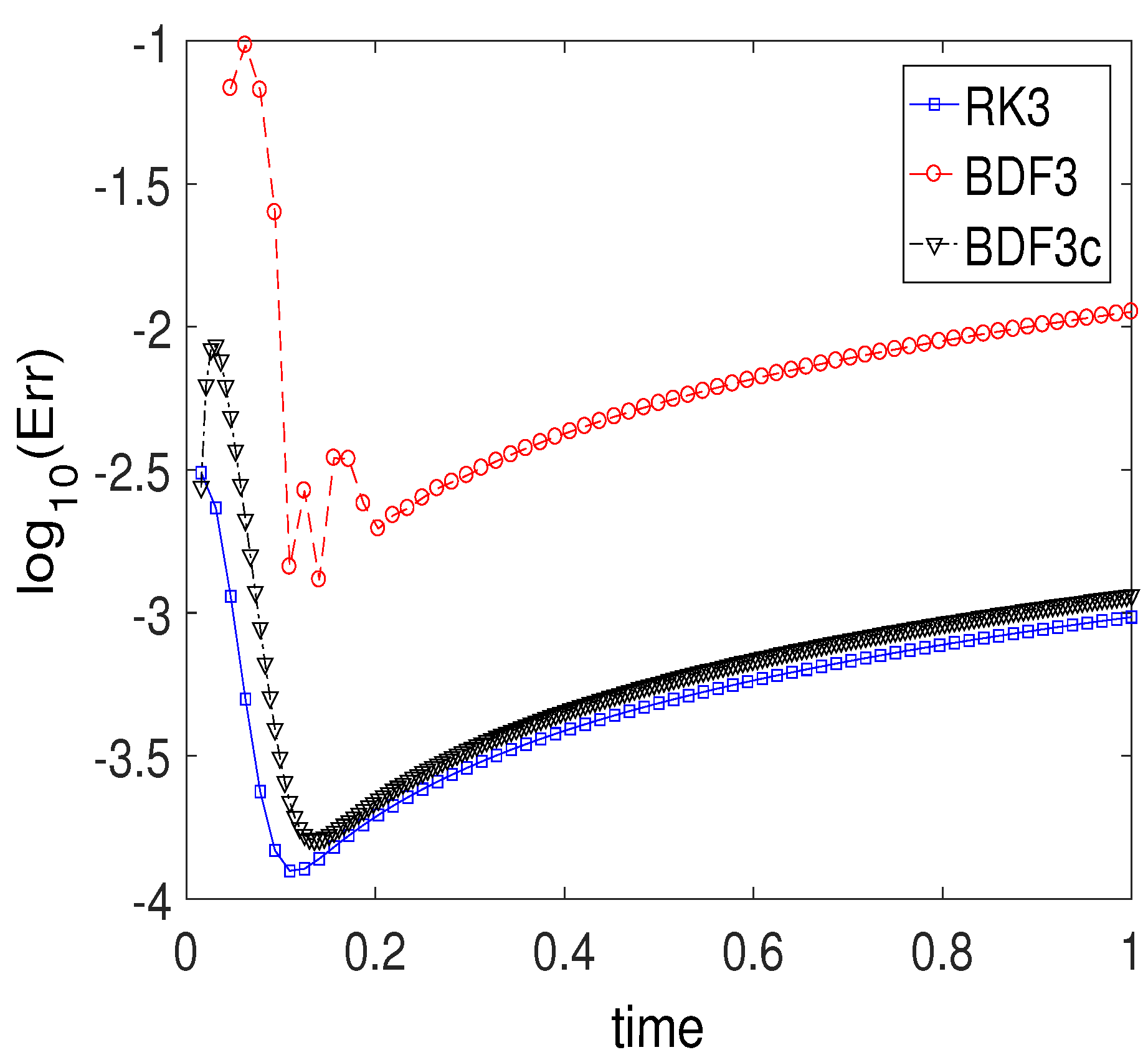
To examine the numerical accuracy of two methods for big size stiff systems, we integrate this problem by setting the system size $N=100$, step size $h=1/64$ for RK3 and step size $\tilde{h}=1/192$ for BDF3. For the numerical comparison, we measure $L_{\infty }$-norm error $Err\left(t_i\right)=\left|\right|u(x_j,t_i)-u_j^i{\left|\right|}_{\infty }$ in each integration time step where $u_j^i\approx u(x_j,t_i)$. The error behaviors of two methods are plotted in Figure 3, which are measured on a logarithmic scale.

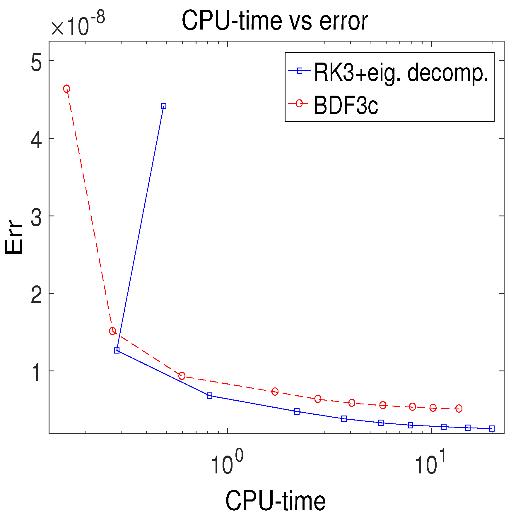
It can be seen that the accuracy of the multi-stage method RK3 with time step h is quite similar to that of the multi-step method BDF3 with time step size $\tilde{h}$. Additionally, to observe of the efficiency for the two methods, CPU-times, and the absolute error are measured at the final time $t=1$ by varying the resolution of space $N=k·{10}^2$ from $k=1$ to $k=10$. The results are plotted by absolute error versus CPU-time in Figure 4 with time step sizes $h=1/100$ and $\tilde{h}=1/300$.

Figure 4 can be good evidence of the conclusion that RK3 with eigenvalue decomposition technique is more efficient than the BDF3 method. More precisely speaking, BDF3 requires more computational costs to obtain a similar magnitude of accuracy. In addition, RK3 combined with the eigenvalue decomposition technique can obtain higher accuracy for the same cost.

3.4. Nonlinear PDE: Medical Akzo Nobel Problem

In this example, we consider one of nonlinear stiff PDE, a reaction-diffusion system with one spatial dimension, described by

$$\begin{array}{c}\hfill \begin{array}{cc}\hfill & \left\{\begin{array}{c}{u}_t=u_{xx}-kuv\hfill \\ v_t=-kuv\hfill \end{array}\right.0<x<\infty ,0<t<T,\hfill \end{array}\end{array}$$

(17)

along with the following initial and boundary conditions,

$$\begin{array}{c}\hfill u(0,x)=0,v(0,x)=v_0\mathrm{for}x>0,\end{array}$$

where $v_0$ is a constant and

$$\begin{array}{c}\hfill u(t,0)=\varphi \left(t\right)\mathrm{for}0<t<T.\end{array}$$

Semi-discretization of this system yields the nonlinear stiff ODE given by

$$\begin{array}{c}\hfill \frac{dy}{dt}=f(t,y),y\left(0\right)=g,y\in {\mathrm{I}\mathrm{R}}^{2N},0\le t\le 20.\end{array}$$

(18)

The function f is given by

$$\begin{array}{c}\hfill \begin{array}{cc}\hfill f_{2j-1}& ={\alpha }_j\frac{y_{2j+1}-y_{2j-3}}{2\Delta \zeta }+{\beta }_j\frac{y_{2j-3}-2y_{2j-1}+y_{2j+1}}{{(\Delta \zeta )}^2}-k{y}_{2j-1}{y}_{2j},\hfill \\ \hfill f_{2j}& =-k{y}_{2j}{y}_{2j-1},\hfill \end{array}\end{array}$$

where

$$\begin{array}{c}\hfill {\alpha }_j=\frac{2{(j\Delta \zeta -1)}^3}{c^2},{\beta }_j=\frac{{(j\Delta \zeta -1)}^4}{c^2},j=1,\dots ,N\end{array}$$

with $\Delta \zeta =\frac{1}{N}$, $y_{-1}\left(t\right)=\varphi \left(t\right)$, $y_{2N+1}=y_{2N-1}$ and

$$\begin{array}{c}\hfill g={(0,v_0,0,v_0,\dots ,0,v_0)}^T\in {\mathrm{I}\mathrm{R}}^{2N}.\end{array}$$

The function $\varphi$ is given by

$$\begin{array}{c}\hfill \varphi \left(t\right)=\left\{\begin{array}{c}2\mathrm{for}t\in (0,5],\hfill \\ 0\mathrm{for}t\in (5,20].\hfill \end{array}\right.\end{array}$$

The parameters k, $v_0$, and c are set to 100, 1, and 4, respectively. The integer N can be decided by the user. In this experiment, we set N as 200. Since analytic solutions are unavailable, we use reference solutions listed in

Table 1. Reference solutions for Medical Akzo Nobel problem at the end of the integration interval.

	Reference Solution		Reference Solution
$y_{79}$	$0.2339942217046434\times {10}^{-3}$	$y_{80}$	$-0.2339942217046434\times {10}^{-141}$
$y_{149}$	$0.3595616017506735\times {10}^{-3}$	$y_{150}$	$0.1649638439865233\times {10}^{-86}$
$y_{199}$	$0.11737412926802\times {10}^{-3}$	$y_{200}$	$0.61908071460151\times {10}^{-5}$
$y_{239}$	$0.68600948191191\times {10}^{-11}$	$y_{240}$	$0.99999973258552$

excerpted from [43].

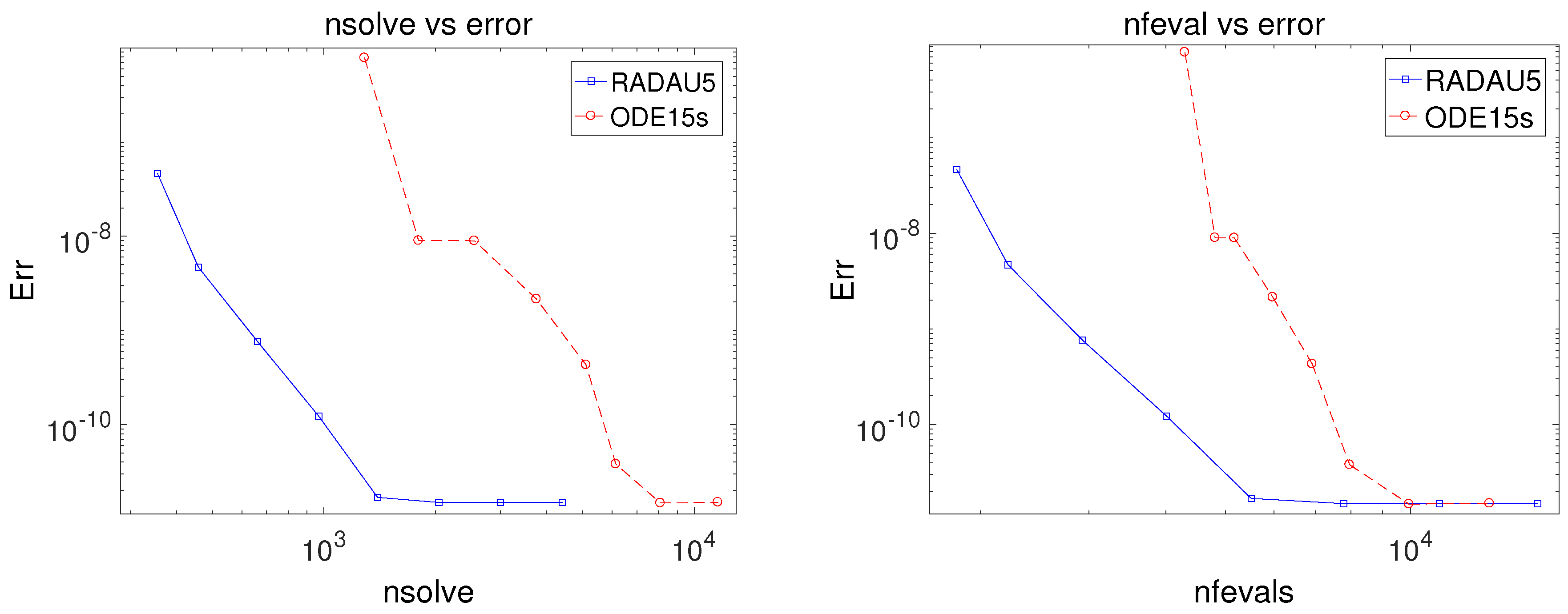
Specifically, results independent of computational resources were measured to compare the efficiency of two methods in this example. The number of times that nonlinear solvers are called (nsolve) and the number of function evaluations (nfeval) are measured by varying relative tolerance ($Rtol$) and absolute tolerance ($Atol$) as $(Rtol,Atol)=({10}^{-n},{10}^{-n-2})(n=4,\dots ,11)$. We also measure an $L_{\infty }$-norm error at the end time for each tolerance and plot the error in a logarithm scale as a function of nsolve (left) and nfeval (right) in Figure 5. These figures show that RADAU5 generates smaller errors, compared with ODE15s, for paying a similar computational expenses. From a different perspective, RADAU5 requires less computational resources than ODE15s to get similar level of errors. Thus, we can claim that RADAU5 has better performance in terms of computational costs and accuracy than ODE15s.

3.5. Kepler Problem

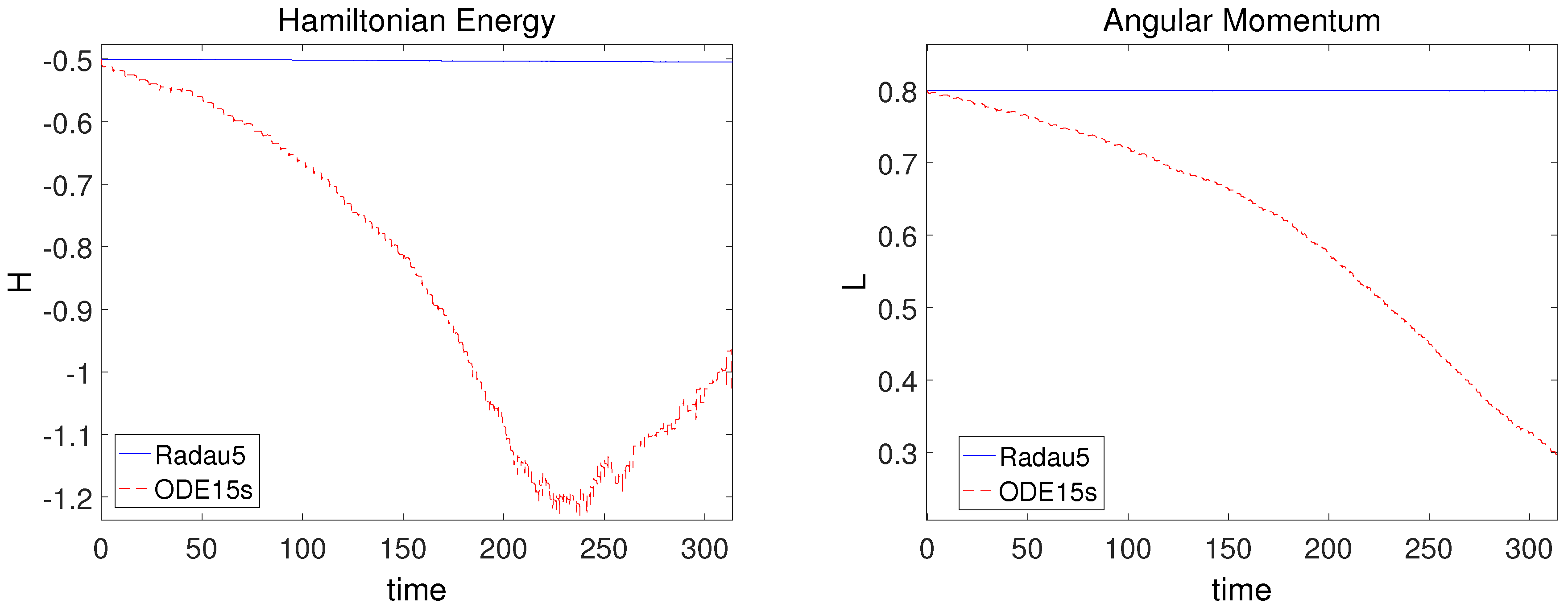
In this subsection, we consider a two-body Kepler’s problem to examine two conservation properties—the Hamiltonian energy and angular momentum—which are indispensable factors in physics. The Kepler’s problem describes the Newton’s law of gravity revolving around their center of mass placed at the origin in elliptic orbits in the $(q_1,q_2)$-plan [44]. The equations with unitary masses and gravitational constant are defined by

$$\begin{array}{c}\hfill \left\{\begin{array}{c}{p}_1^{\prime }\left(t\right)=-q_1{(q_1^2+q_2^2)}^{(-3/2)},\hfill \\ p_2^{\prime }\left(t\right)=-q_2{(q_1^2+q_2^2)}^{(-3/2)},\hfill \\ q_1^{\prime }\left(t\right)=p_1,\hfill \\ q_2^{\prime }\left(t\right)=p_2,\hfill \end{array}\right.\end{array}$$

(19)

with initial conditions $p_1\left(0\right)=0$, $p_2\left(0\right)=2$, $q_1\left(0\right)=0.4$, and $p_1\left(0\right)=0$ on the interval $[0,100\pi ]$. The dynamics are described by Hamiltonian function given by

$$\begin{array}{c}\hfill H(p_1,p_2,q_1,q_2)=\frac{1}{2}(p_1^2+p_2^2)-\frac{1}{\sqrt{q_1^2+q_2^2}}\end{array}$$

together with angular momentum L given by

$$\begin{array}{c}\hfill L(p_1,p_2,q_1,q_2)=q_1{p}_2-q_2{p}_1.\end{array}$$

The initial Hamiltonian and the initial angular momentum conditions are $H_0=-0.5$ and $L_0=0.8$, respectively.

The conservation properties for the Hamiltonian energy H and angular momentum L are investigated by simulating with the two methods, RADAU5 and ODE15s, with time step size $h=0.1$ and plot the results in Figure 6. As shown in Figure 6, RADAU5 can conserve both quantities, whereas ODE15s loses the properties as time is going on.

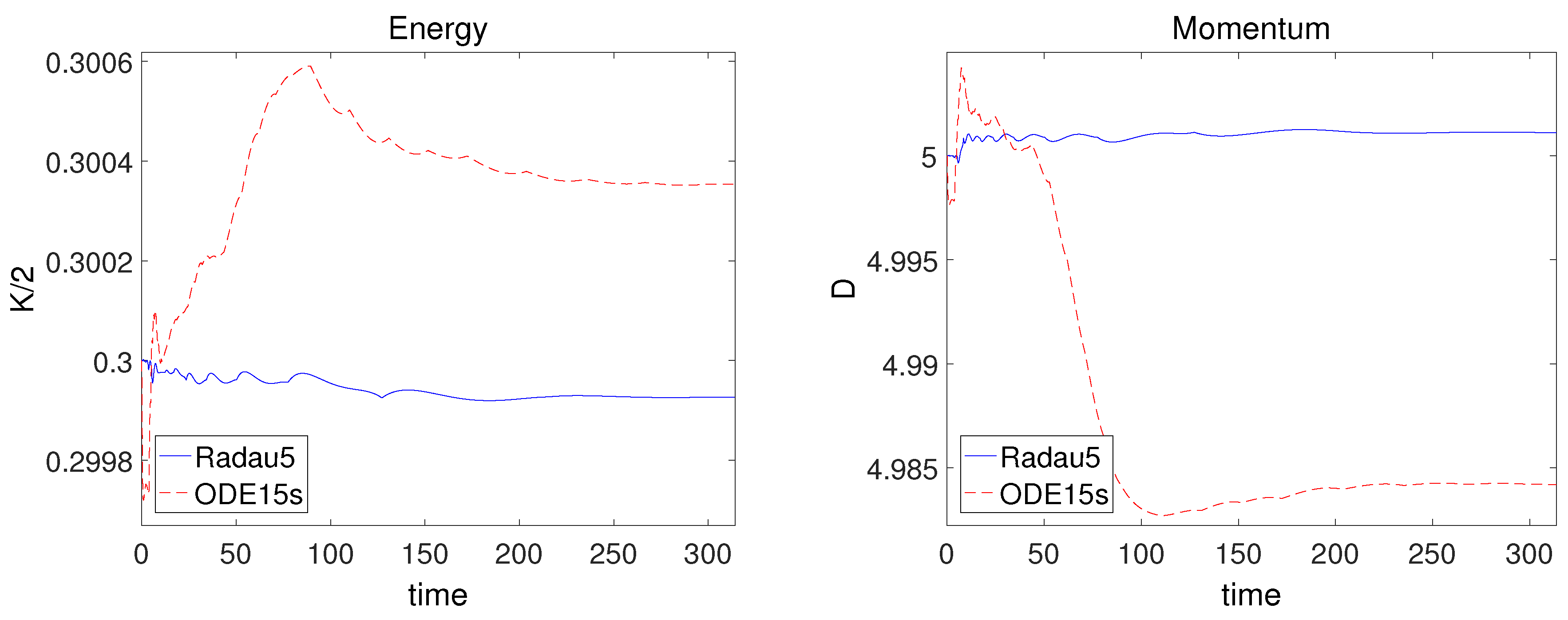
Next, we also consider the movement of comet in planar regulated three-body problem of Sun–Jupiter–Comet. To investigate conservation properties of the two methods, we measure the Hamiltonian energy K and the angular momentum D for the three-body Kepler problem described by

$$\begin{array}{c}\hfill x^{″}\left(t\right)=\nu \frac{x_S-x}{r_{13}^3}+\mu \frac{x_J-x}{r_{23}^3},y^{″}\left(t\right)=\nu \frac{y_S-y}{r_{13}^3}+\mu \frac{y_J-y}{r_{23}^3},\end{array}$$

(20)

where

$$\begin{array}{cc}\hfill & r_{13}^2={(x_S-x)}^2+{(y_S-y)}^2,r_{23}^2={(x_J-x)}^2+{(y_J-y)}^2,\hfill \\ \hfill & x_S=-\mu cos(t-t_0),y_S=-\mu sin(t-t_0),\hfill \\ \hfill & x_J=\nu cos(t-t_0),y_J=\nu sin(t-t_0).\hfill \end{array}$$

The energy and angular momentum of the comet

$$\begin{array}{c}\hfill K/2=\frac{1}{2}(x^2+y^2)-\frac{1}{\sqrt{x^2+y^2}},D=x{y}^{\prime }-y{x}^{\prime }\end{array}$$

are constant, when $\mu =0$ and $\nu =1$. For this experiment, initial condition is set to

$$\begin{array}{c}\hfill x\left(0\right)=5,y\left(0\right)=1,x^{\prime }\left(0\right)=0,y^{\prime }\left(0\right)=1,\end{array}$$

and the initial energy and angular momentum are set to $K_0/2=0.3$ and $D_0=5$ with parameter step size $h=1/2\pi$ and $t_0=0$.

In Figure 7, one can see that the behaviors of the energy and the momentum over time interval $[0,100\pi ]$. As observed in Figure 7, RADAU5 gives a maximum variation of $8.0356\times {10}^{-5}$ and $0.0013$ for the energy and the momentum, whereas ODE15s presents a variation of $5.9063\times {10}^{-4}$ and $0.0173$ for them. Therefore, one can conclude that RADAU5 has better conservation properties, compared with ODE15s.

4. Conclusions and Further Discussion

In this work, we compare multi-stage methods with multi-step methods by investigating the numerical properties of both methods. In a classical approach, nonlinear stiff systems were usually solved by multi-step methods to avoid huge computational complexity induced from linearization of a given nonlinear system. However, the computational costs for the multi-stage method can be reduced sufficiently without loss of stability and conservation, which is possible by using suitable nonlinear and linear solvers such as a Newton-type method and eigenvalue decomposition. It means that the multi-stage method can also be applied to solve nonlinear stiff systems without any damage to computational costs, compared with the multi-step methods. Moreover, it is seen that the multi-stage methods preserve the invariants of the energy and angular momentum in Hamiltonian systems. In addition, it is well-known that a stability property of multi-stage methods is much better than that of multi-step methods.

Overall, one can conclude that the multi-stage method can be a good candidate to solve nonlinear stiff systems. It means that, without any damage to computational costs, multi-stage methods can be applied to long-time simulations and massive physical simulations in fields such as astronomy, meteorology, nuclear fusion, nuclear power, aerospace, machinery, etc.

References

1. Atkinson, K.E. Divisions of numerical methods for ordinary differential equations. In An Introduction to Numerical Analysis, 2nd ed.; John Wiley & Sons, Inc.: Hoboken, NJ, USA, 1989; pp. 333–462. [Google Scholar]
2. Gear, C.W. Numerical Initial Value Problems in Ordinary Differential Equations; Prentice Hall: Upper Saddle River, NJ, USA, 1971. [Google Scholar]
3. Hairer, E.; Nørsett, S.P.; Wanner, G. Solving Ordinary Differential Equations I: Nonstiff Problems; Springer: Berlin/Heidelberg, Germany; New York, NY, USA, 1996. [Google Scholar]
4. Kirchgraber, U. Multi-step Method Are Essentially One-step Methods. Numer. Math. 1986, 48, 85–90. [Google Scholar] [CrossRef]
5. Alolyan, I.; Simos, T.E. New multiple stages multistep method with best possible phase properties for second order initial/boundary value problems. J. Math. Chem. 2019, 57, 834–857. [Google Scholar] [CrossRef]
6. Berg, D.B.; Simos, T.E. Three stages symmetric six-step method with eliminated phase-lag and its derivatives for the solution of the Schrödinger equation. J. Chem. Phys. 2017, 55, 1213–1235. [Google Scholar] [CrossRef]
7. Butcher, J.C. Numerical Analysis of Ordinary Differential Equations: Runge–Kutta and General Linear Methods; John Wiley & Sons, Inc.: Hoboken, NJ, USA, 1987. [Google Scholar]
8. Enright, W.; Hull, T.; Lindberg, B. Comparing numerical methods for stiff systems of O.D.E.’s. BIT Numer. Math. 1975, 15, 10–48. [Google Scholar] [CrossRef]
9. Fathoni, M.F.; Wuryandari, A.I. Comparison between Euler, Heun, Runge–Kutta and Adams-Bashforth Moulton integration methods in the particle dynamic simulation. In Proceedings of the 2015 4th International Conference on Interactive Digital Media (ICIDM), Bandung, Indonesia, 1–5 December 2015; pp. 1–7. [Google Scholar]
10. Liniger, W.; Willoughby, R.A. Efficient Integration Methods for Stiff Systems of Ordinary Differential Equations. SIAM J. Numer. Anal. 1970, 7, 47–66. [Google Scholar] [CrossRef]
11. Song, X. Parallel Multi-stage and Multi-step Method in ODEs. J. Comput. Math. 2000, 18, 157–164. [Google Scholar]
12. Barrio1, M.; Burrage, K.; Burrage, P. Stochastic linear multistep methods for the simulation of chemical kinetics. J. Chem. Phys. 2015, 142, 064101. [Google Scholar] [CrossRef]
13. Bu, S. New construction of higher-order local continuous platforms for Error Correction Methods. J. Appl. Anal. Comput. 2016, 6, 443–462. [Google Scholar]
14. Cohen, E.B. Analysis of a Class of Multi-stage, Multi-step Runge Kutta Methods. Comput. Math. Appl. 1994, 27, 103–116. [Google Scholar] [CrossRef]
15. Guo, L.; Zeng, F.; Turner, I.; Burrage, K.; Karniadakis, G.E. Efficient multistep methods for tempered fractional calculus: Algorithms and Simulations. SIAM J. Sci. Comput. 2019, 41, A2510–A2535. [Google Scholar] [CrossRef]
16. Han, T.M.; Han, Y. Solving Implicit Equations Arising from Adams-Moulton Methods. BIT Numer. Math. 2002, 42, 336–350. [Google Scholar] [CrossRef]
17. Ghawadri, N.; Senu, N.; Fawzi, F.A.; Ismail, F.; Ibrahim, Z.B. Explicit Integrator of Runge–Kutta Type for Direct Solution of u(4) = f(x, u, ú, ü). Symmetry 2019, 10, 246. [Google Scholar] [CrossRef]
18. Kim, S.D.; Kwon, J.; Piao, X.; Kim, P. A Chebyshev Collocation Method for Stiff Initial Value Problems and Its Stability. Kyungpook Math. J. 2011, 51, 435–456. [Google Scholar] [CrossRef]
19. Kim, P.; Piao, X.; Jung, W.; Bu, S. A new approach to estimating a numerical solution in the error embedded correction framework. Adv. Differ. Equ. 2018, 68, 1–21. [Google Scholar] [CrossRef]
20. Kim, P.; Kim, J.; Jung, W.; Bu, S. An Error Embedded Method Based on Generalized Chebyshev Polynomials. J. Comput. Phys. 2016, 306, 55–72. [Google Scholar] [CrossRef]
21. Piao, X.; Bu, S.; Kim, D.; Kim, P. An embedded formula of the Chebyshev collocation method for stiff problems. J. Comput. Phys. 2017, 351, 376–391. [Google Scholar] [CrossRef]
22. Xia, K.; Cong, Y.; Sun, G. Symplectic Runge–Kutta methods of high order based on W-transformation. J. Appl. Anal. Comput. 2001, 3, 1185–1199. [Google Scholar]
23. Marin, M. Effect of microtemperatures for micropolar thermoelastic bodies. Struct. Eng. Mech. 2017, 61, 381–387. [Google Scholar] [CrossRef]
24. Marin, M.; Abd-Alla, A.; Raducanu, D.; Abo-Dahab, S. Structural Continuous Dependence in Micropolar Porous Bodies. Comput. Mater. Contin. 2015, 45, 107–125. [Google Scholar]
25. Bak, S. High-order characteristic-tracking strategy for simulation of a nonlinear advection-diffusion equations. Numer. Methods Partial Differ. Equ. 2019, 35, 1756–1776. [Google Scholar] [CrossRef]
26. Dahlquist, G. Numerical integration of ordinary differential equations. Math. Scand. 1956, 4, 33–50. [Google Scholar] [CrossRef]
27. Pazner, W.; Persson, P. Stage-parallel fully implicit Runge–Kutta solvers for discontinuous Galerkin fluid simulationse. J. Comput. Phys. 2017, 335, 700–717. [Google Scholar] [CrossRef]
28. Piao, X.; Kim, P.; Kim, D. One-step L (α)-stable temporal integration for the backward semi-Lagrangian method and its application in guiding center problems. J. Comput. Phys. 2018, 366, 327–340. [Google Scholar] [CrossRef]
29. Prothero, A.; Robinson, A. On the Stability and Accuracy of One-step Methods for Solving Stiff Systems of Ordinary Differential Equations. Math. Comput. 1974, 28, 145–162. [Google Scholar] [CrossRef]
30. Bickart, T.A. An Efficient Solution Process for Implicit Runge–Kutta Methods. SIAM J. Numer. Anal. 1977, 14, 1022–1027. [Google Scholar] [CrossRef]
31. Butcher, J.C. On the Implementation of Implicit Runge–Kutta Methods. BIT Numer. Math. 1976, 16, 237–240. [Google Scholar] [CrossRef]
32. Curtiss, C.F.; Hirschfelder, J.O. Integration of Stiff Equations. Proc. Natl. Acad. Sci. USA 1952, 38, 235–243. [Google Scholar] [CrossRef]
33. Jeon, Y.; Bu, S.; Bak, S. A comparison of multi-Step and multi-stage methods. Int. J. Circuits Signal Process. 2017, 11, 250–253. [Google Scholar]
34. Coper, G.J.; Butcher, J.C. An iteration method for implicit Runge–Kutta methods. IMA J. Numer. Anal. 1983, 3, 127–140. [Google Scholar] [CrossRef]
35. Cooper, G.J.; Vignesvaran, R. Some methods for the implementation of implicit Runge–Kutta methods. J. Comput. Appl. Math. 1993, 45, 213–225. [Google Scholar] [CrossRef]
36. Frank, R.; Ueberhuber, C.W. Iterated defect correction for the efficient solution of stiff systems of ordinary differential equations. BIT Numer. Math. 1977, 17, 146–159. [Google Scholar] [CrossRef]
37. Gonzalez-Pinto, S.; Rojas-Bello, R. Speeding up Newton-type iterations for stiff problems. J. Comput. Appl. Math. 2005, 181, 266–279. [Google Scholar] [CrossRef]
38. Hairer, E.; Wanner, G. Solving Ordinary Differential Equations II: Stiff and Differential Algebraic Problems; Springer: Berlin/Heidelberg, Germany; New York, NY, USA, 1996. [Google Scholar]
39. Huang, J.; Jia, J.; Minion, M.L. Accelerating the convergence of spectral deferred correction methods. J. Comput. Phys. 2006, 214, 633–656. [Google Scholar] [CrossRef]
40. Süli, E.; Mayers, D.F. An Introduction to Numerical Analysis; Cambridge University Press: Cambridge, UK, 2003. [Google Scholar]
41. Dahlquist, G. A special stability problem for linear multistep methods. BIT Numer. Math. 1963, 3, 27–43. [Google Scholar] [CrossRef]
42. Shampine, L.F.; Reichelt, M.W. The MATLAB ODE Suite. SIAM J. Sci. Comput. 1997, 18, 1–22. [Google Scholar] [CrossRef]
43. Mazzia, F.; Magherini, C. Test Set for Initial Value Problem Solvers; Department of Mathematics, University of Bari: Bari, Italy, 2008. [Google Scholar]
44. Brugnano, L.; Iavernaro, F.; Trigiante, D. Energy- and Quadratic Invariants–Preserving Integrators Based upon Gauss Collocation Formulae. SIAM J. Numer. Anal. 2012, 50, 2897–2916. [Google Scholar] [CrossRef] [Green Version]
Figure 1. Prothero–Robinson equation: comparing two methods for accuracy by varying step size h = 2 k , for (a) k = 1 , (b) k = 2 , (c) k = 3 .
Mathematics 07 01158 g001
Figure 2. Multi-mode problem: comparing errors of two methods for linear case (left) and nonlinear case (right).
Mathematics 07 01158 g002
Figure 3. Heat equation: comparing two methods for error behaviors over time.
Mathematics 07 01158 g003
Figure 4. Heat equation: comparing two methods for CPU-time versus error.
Mathematics 07 01158 g004
Figure 5. Medical Akzo Nobel problem: nsolve versus error (left) and nfeval versus error (right).
Mathematics 07 01158 g005
Figure 6. Two-body Kepler problem: comparing two methods in terms of conservation of Hamiltonian and angular momentum.
Mathematics 07 01158 g006
Figure 7. Three-body Kepler problem: comparing two methods in terms of the conservation of total energy and angular momentum.
Mathematics 07 01158 g007