A New Hybrid Evolutionary Algorithm for the Treatment of Equality Constrained MOPs


 and
and 
Abstract
1. Introduction
2. Background and Related Work
2.1. Multi-Objective Optimization Problem (MOP)
2.2. Related Work
- The hybridization scheme, which can consists on seeding the initial population of the MOEA [34], interleaving global and local search steps by applying local search to some selected individuals of the population [33] or periodically (every t generations) [35], or using the non-dominated solutions obtained by the exact algorithm to reconstruct the whole Pareto front [36].
2.3. Test Suites for Constrained MOPs
2.4. Pareto Tracer (PT)
3. Proposed Test Problems
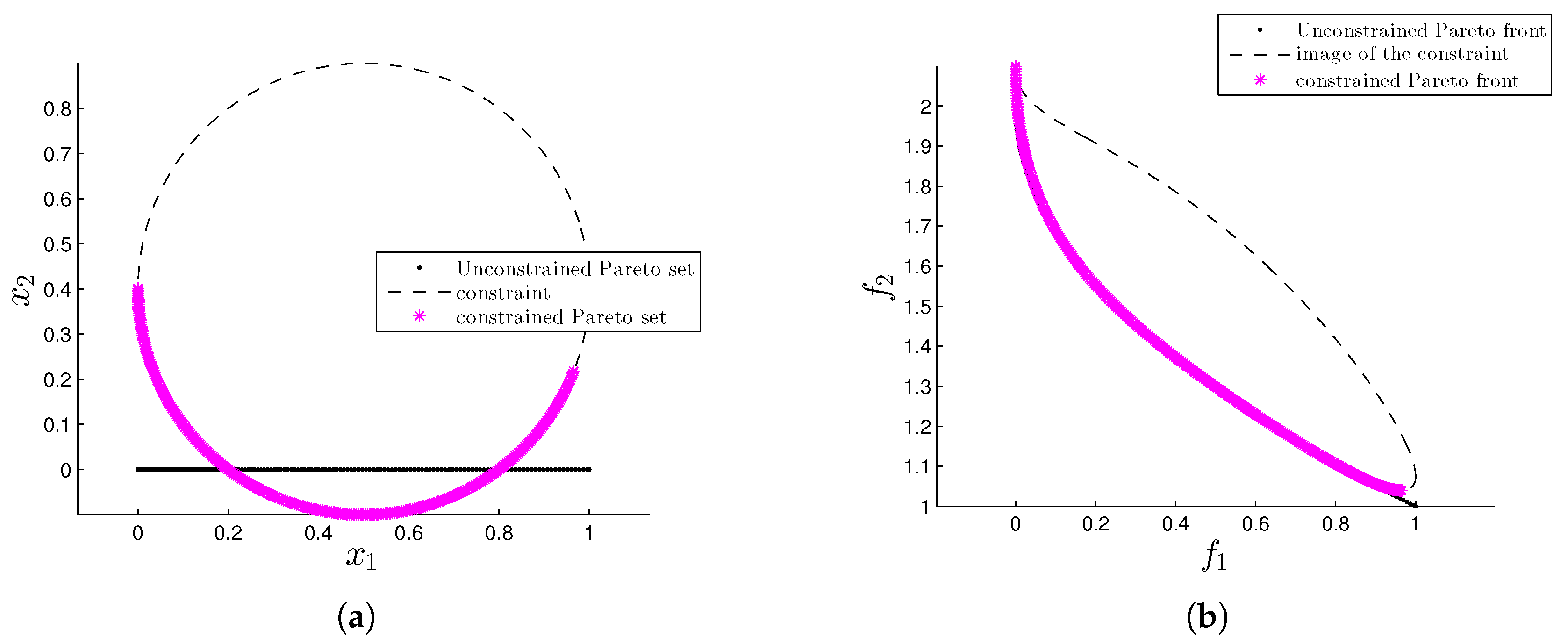
3.1. Eq1-ZDT1
- For the first objective we have that .
- For the second objective we have thatThen,Finally,which contradicts the hypothesis. Thus with .
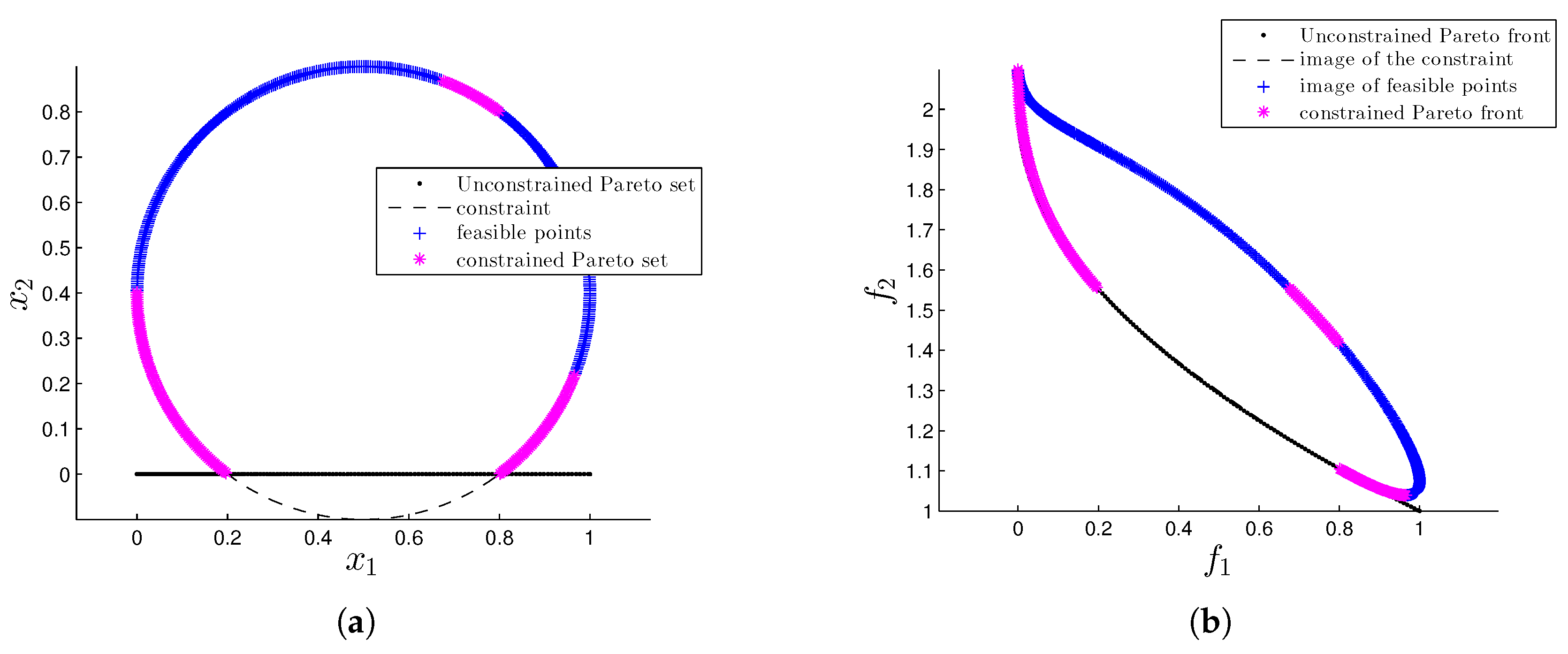
3.2. Eq2-ZDT1
- (a)
- (b)
- As second step, we need to remove all the points in that do not satisfy the box constraints. In particular, as , we focus on and . For , we have that and , i.e., some values of do not satisfy the lower bound.We can express as follows:thus, for we can find the values of that define and via:After removing the non-feasible points from we have a gap in Pareto set/front. Now, notice that, some points (that is, ), could be within the gap. That is, we have to find the values of such that .For this we consider:where, .Notice that and is a continuous function, then for the intermediate value theorem such that and , respectively.For , such values are and . Then , with , as and .
3.3. Eq-Quad
4. Proposed Algorithm (-NSGA-IIPT)
4.1. First Stage: Rough Approximation via -NSGA-II
- –
- the number of solutions in the roughly approximated set is small, in order to reduce the computational burden of the local search (PT). Indeed, in case of a completely connected front, one single approximated solution might allow us to build the entire Pareto front.
- –
- the MOEA should promote diversity, since the rough approximation produced should cover all the extent of the Pareto front and identify all the different components, in case of a disconnected front.
- –
- the MOEA must be able to handle equality constraints. As mentioned before, a severely constrained problem might cause diversity issues that should be overcome by the MOEA.
4.2. Second Stage: Refinement via PT
- Let be the desired minimal distance between two solutions in objective space. In this first step, go over P and eliminate elements that are too close to each other (if needed). This leads to the new archive .
- Apply the Newton method (A11) to all elements of . Remove all dominated solutions, and elements that are too close to each other as in the first step. This leads to the archive .
- To obtain a “global picture” of the part of the Pareto front that will be computed by PT, construct a partition of a potentially interesting subset S of the image space into a set of hyper-cubes (or k-dimensional boxes) with radius . This partition can easily be constructed via using a binary tree whose root represents S (see [45] for details, where, however, the partition is used in decision variable space). S is a box that is constructed out of as follows: denote by and the minimal and maximal value of the i-th objective value of all elements in , respectively. Then the i-th element of the center of S is set to and its i-th element of the radius to . In the computations, we will only allow a storing one candidate solution within each of these boxes in the archive A to guarantee a spread of the solutions.
| Algorithm 1:-NGSA-II |
| Evaluate each individual to obtain and |
| Compute and set |
| for to do |
| ▹ Parent selection through tournament and -constraint |
| , |
| Fill P with , using crowding distance if necessary |
| if then |
| Complete P with |
| end if |
| Update through Equation (21) |
| end for |
| ▹ return 20 solutions |
| Return P and |
- if is dominated by any element of A, then PT the current application of PT is stopped.
- else, it is checked if the unique box that contains is already contained in C. If this is not the case, add this box to C and add to A. Else, decline and proceed with .
5. Numerical Results
5.1. Performance Assessment
5.2. Solving Equality Constrained MOPs with Mathematical Programming Techniques
5.3. Solving Equality Constrained MOPs with MOEAs
- NSGA-II. The popular non-dominated sorting genetic algorithm II [50] was adopted in our comparative study. NSGA-II employs a binary tournament-based on feasibility in the mating selection procedure. In order to determine the next generation, the crowding comparison operator considers the feasibility of solutions. In our study, NSGA-II was performed using the standard parameters given by its authors, i.e., .
- GDE3. The third evolution step of generalized differential evolution [51] was also adopted in our experimental analysis. GDE3 introduces the concept of constraint-domination explained before to discriminate solutions. GDE3 was employed using and .
- cMOEA/D-DE. We also adopted the first version of the multi-objective evolutionary algorithm based on decomposition for constraint multi-objective optimization [52]. cMOEA/D-DE utilizes a penalty function in order to satisfy the constraint of the problem. The penalty function is straightforward added to the scalarizing function employed by MOEA/D-DE [53] to approximate the PF of a constrained MOP. cMOEA/D-DE was employed using , and .
- eMOEA/D-DE. A version of MOEA/D-DE based on the -constraint method for constrained optimization [54] is also adopted in our experimental study. eMOEA/D-DE employs the -constraint method to satisfy the constraints of the problem by obtaining information about feasible solutions in the neighborhood of MOEA/D-DE. Thus, the neighboring solutions are used to defined the -constraint value which is dynamically adapted during the search process of eMOEA/D-DE. eMOEA/D-DE was performed using the standard parameters suggested by its authors, i.e., , and .
5.4. Analysis
6. Conclusions
Author Contributions
Funding
Acknowledgments
Conflicts of Interest
Appendix A. Pareto Tracer (PT)
Appendix B. Graphical Results for the NBI

Appendix C. Graphical results for the ϵ-NSGAII/PT

Appendix D. Values of γ and η

| n | ||
|---|---|---|
| 16 | 0.954380 | 0.863336 |
| 17 | 0.957029 | 0.848048 |
| 18 | 0.959445 | 0.832853 |
| 19 | 0.961656 | 0.817805 |
| 20 | 0.963686 | 0.802946 |
| 21 | 0.965554 | 0.788312 |
| 22 | 0.967278 | 0.773932 |
| 23 | 0.968874 | 0.759830 |
| 24 | 0.970353 | 0.746025 |
| 25 | 0.971727 | 0.732530 |
| 26 | 0.973006 | 0.719359 |
| 27 | 0.974199 | 0.706518 |
| 28 | 0.975314 | 0.694012 |
| 29 | 0.976357 | 0.681847 |
| 30 | 0.977336 | 0.670021 |
| 31 | 0.978253 | 0.658536 |
| 32 | 0.979116 | 0.647389 |
References
- Kalyanmoy, D. Multi Objective Optimization Using Evolutionary Algorithms; John Wiley and Sons: Hoboken, NJ, USA, 2001. [Google Scholar]
- Coello, C.A.C.; Lamont, G.B.; Van Veldhuizen, D.A. Evolutionary Algorithms for Solving Multi-Objective Problems; Springer: Cham, Switzerland, 2007; Volume 5. [Google Scholar]
- Ullah, A.S.B.; Sarker, R.; Lokan, C. Handling equality constraints in evolutionary optimization. Eur. J. Oper. Res. 2012, 221, 480–490. [Google Scholar] [CrossRef]
- Ponsich, A.; Jaimes, A.L.; Coello, C.A.C. A Survey on Multiobjective Evolutionary Algorithms for the Solution of the Portfolio Optimization Problem and Other Finance and Economics Applications. IEEE Trans. Evol. Comput. 2013, 17, 321–344. [Google Scholar] [CrossRef]
- Chen, X.L.; Wang, P.H.; Wang, Q.; Dong, Y.H. A Two-Stage strategy to handle equality constraints in ABC-based power economic dispatch problems. Soft Comput. 2019, 23, 6679–6696. [Google Scholar] [CrossRef]
- Liao, Z.; Rittscher, J. A multi-objective supplier selection model under stochastic demand conditions. Int. J. Prod. Econ. 2007, 105, 150–159. [Google Scholar] [CrossRef]
- Bernardino, H.S.; Barbosa, H.J.C.; Angelo, J.S. Differential Evolution with Adaptive Penalty and Tournament Selection for Optimization Including Linear Equality Constraints. In Proceedings of the 2018 IEEE Congress on Evolutionary Computation (CEC), Rio de Janeiro, Brazil, 8–13 July 2018; pp. 1–8. [Google Scholar] [CrossRef]
- Barbosa, H.J.C.; Bernardino, H.S.; Angelo, J.S. An improved differential evolution algorithm for optimization including linear equality constraints. Memetic Comput. 2018, 11, 317–329. [Google Scholar] [CrossRef]
- Ghannadpour, S.F.; Noori, S.; Tavakkoli-Moghaddam, R.; Ghoseiri, K. A multi-objective dynamic vehicle routing problem with fuzzy time windows: Model, solution and application. Appl. Soft Comput. 2014, 14, 504–527. [Google Scholar] [CrossRef]
- Cuate, O.; Uribe, L.; Lara, A.; Schütze, O. A benchmark for equality constrained multi-objective optimization. Swarm Evol. Comput. 2020, 52, 100619. [Google Scholar] [CrossRef]
- Martín, A.; Schütze, O. Pareto Tracer: A predictor–corrector method for multi-objective optimization problems. Eng. Optim. 2018, 50, 516–536. [Google Scholar] [CrossRef]
- Cuate, O.; Uribe, L.; Ponsich, A.; Lara, A.; Beltran, F.; Sánchez, A.R.; Schütze, O. A New Hybrid Metaheuristic for Equality Constrained Bi-objective Optimization Problems. In Evolutionary Multi-Criterion Optimization; Deb, K., Goodman, E., Coello Coello, C.A., Klamroth, K., Miettinen, K., Mostaghim, S., Reed, P., Eds.; Springer International Publishing: Cham, Switzerland, 2019; pp. 53–65. [Google Scholar]
- Jan, M.A.; Khanum, R.A. A study of two penalty-parameterless constraint handling techniques in the framework of MOEA/D. Appl. Soft Comput. 2013, 13, 128–148. [Google Scholar] [CrossRef]
- Zhang, Q.; Li, H. MOEA/D: A Multiobjective Evolutionary Algorithm Based on Decomposition. IEEE Trans. Evol. Comput. 2007, 11, 712–731. [Google Scholar] [CrossRef]
- Runarsson, T.P.; Yao, X. Stochastic ranking for constrained evolutionary optimization. IEEE Trans. Evol. Comput. 2000, 4, 284–294. [Google Scholar] [CrossRef]
- Deb, K.; Pratap, A.; Agarwal, S.; Meyarivan, T. A fast and elitist multiobjective genetic algorithm: NSGA-II. IEEE Trans. Evol. Comput. 2002, 6, 182–197. [Google Scholar] [CrossRef]
- Deb, K.; Pratap, A.; Meyarivan, T. Constrained Test Problems for Multi-objective Evolutionary Optimization. In Evolutionary Multi-Criterion Optimization; Zitzler, E., Thiele, L., Deb, K., Coello Coello, C.A., Corne, D., Eds.; Springer: Berlin/Heidelberg, Germany, 2001; pp. 284–298. [Google Scholar]
- Zhang, Q.; Zhou, A.; Zhao, S.; Suganthan, P.N.; Liu, W.; Tiwari, S. Multiobjective optimization test instances for the CEC 2009 special session and competition. In Special Session on Performance Assessment of Multi-Objective Optimization Algorithms; Technical Report; University of Essex: Colchester, UK; Nanyang Technological University: Singapore, 2008; Volume 264. [Google Scholar]
- Ray, T.; Singh, H.K.; Isaacs, A.; Smith, W. Infeasibility Driven Evolutionary Algorithm for Constrained Optimization. In Constraint-Handling in Evolutionary Optimization; Mezura-Montes, E., Ed.; Springer: Berlin/Heidelberg, Germany, 2009; pp. 145–165. [Google Scholar] [CrossRef]
- Liu, M.; Zou, X.; Chen, Y.; Wu, Z. Performance assessment of DMOEA-DD with CEC 2009 MOEA competition test instances. In Proceedings of the 2009 IEEE Congress on Evolutionary Computation, Trondheim, Norway, 18–21 May 2009; pp. 2913–2918. [Google Scholar] [CrossRef]
- Isaacs, A.; Ray, T.; Smith, W. Blessings of maintaining infeasible solutions for constrained multi-objective optimization problems. In Proceedings of the 2008 IEEE Congress on Evolutionary Computation (IEEE World Congress on Computational Intelligence), Hong Kong, China, 1–6 June 2008; pp. 2780–2787. [Google Scholar] [CrossRef]
- Asafuddoula, M.; Ray, T.; Sarker, R.; Alam, K. An adaptive constraint handling approach embedded MOEA/D. In Proceedings of the 2012 IEEE Congress on Evolutionary Computation, Brisbane, QLD, Australia, 10–15 June 2012; pp. 1–8. [Google Scholar] [CrossRef]
- Fan, Z.; Li, H.; Wei, C.; Li, W.; Huang, H.; Cai, X.; Cai, Z. An improved epsilon constraint handling method embedded in MOEA/D for constrained multi-objective optimization problems. In Proceedings of the 2016 IEEE Symposium Series on Computational Intelligence (SSCI), Athens, Greece, 6–9 December 2016; pp. 1–8. [Google Scholar] [CrossRef]
- Takahama, T.; Sakai, S. Constrained Optimization by the ϵ Constrained Differential Evolution with Gradient-Based Mutation and Feasible Elites. In Proceedings of the 2006 IEEE International Conference on Evolutionary Computation, Vancouver, BC, Canada, 16–21 July 2006; pp. 1–8. [Google Scholar] [CrossRef]
- Fan, Z.; Li, W.; Cai, X.; Huang, H.; Fang, Y.; You, Y.; Mo, J.; Wei, C.; Goodman, E. An improved epsilon constraint-handling method in MOEA/D for CMOPs with large infeasible regions. Soft Comput. 2019, 23, 12491–12510. [Google Scholar] [CrossRef]
- Fan, Z.; Fang, Y.; Li, W.; Lu, J.; Cai, X.; Wei, C. A comparative study of constrained multi-objective evolutionary algorithms on constrained multi-objective optimization problems. In Proceedings of the 2017 IEEE Congress on Evolutionary Computation (CEC), San Sebastian, Spain, 5–8 June 2017; pp. 209–216. [Google Scholar] [CrossRef]
- Ishibuchi, H.; Fukase, T.; Masuyama, N.; Nojima, Y. Dual-grid Model of MOEA/D for Evolutionary Constrained Multiobjective Optimization. In Proceedings of the Genetic and Evolutionary Computation Conference, Kyoto, Japan, 15–19 July 2018; ACM: New York, NY, USA, 2018; pp. 665–672. [Google Scholar] [CrossRef]
- Jain, H.; Deb, K. An Evolutionary Many-Objective Optimization Algorithm Using Reference-Point Based Nondominated Sorting Approach, Part II: Handling Constraints and Extending to an Adaptive Approach. IEEE Trans. Evol. Comput. 2014, 18, 602–622. [Google Scholar] [CrossRef]
- Ono, S.; Nakayama, S. Multi-Objective Particle Swarm Optimization for robust optimization and its hybridization with gradient search. In Proceedings of the 2009 IEEE Congress on Evolutionary Computation, Trondheim, Norway, 18–21 May 2009; pp. 1629–1636. [Google Scholar] [CrossRef]
- Shim, V.A.; Tan, K.C.; Tan, K.K. A hybrid adaptive evolutionary algorithm in the domination-based and decomposition-based frameworks of multi-objective optimization. In Proceedings of the 2012 IEEE Congress on Evolutionary Computation, Brisbane, QLD, Australia, 10–15 June 2012; pp. 1–8. [Google Scholar] [CrossRef]
- Sindhya, K.; Miettinen, K.; Deb, K. A Hybrid Framework for Evolutionary Multi-Objective Optimization. IEEE Trans. Evol. Comput. 2013, 17, 495–511. [Google Scholar] [CrossRef]
- Martínez, S.Z.; Coello Coello, C.A. A direct local search mechanism for decomposition-based multi-objective evolutionary algorithms. In Proceedings of the 2012 IEEE Congress on Evolutionary Computation, Brisbane, QLD, Australia, 10–15 June 2012; pp. 1–8. [Google Scholar] [CrossRef]
- Hu, X.; Huang, Z.; Wang, Z. Hybridization of the multi-objective evolutionary algorithms and the gradient-based algorithms. In Proceedings of the 2003 Congress on Evolutionary Computation, Canberra, ACT, Australia, 8–12 December 2003; Volume 2, pp. 870–877. [Google Scholar] [CrossRef]
- Hernandez-Diaz, A.G.; Coello Coello, C.A.; Perez, F.; Caballero, R.; Molina, J.; Santana-Quintero, L.V. Seeding the initial population of a multi-objective evolutionary algorithm using gradient-based information. In Proceedings of the 2008 IEEE Congress on Evolutionary Computation (IEEE World Congress on Computational Intelligence), Hong Kong, China, 1–6 June 2008; pp. 1617–1624. [Google Scholar] [CrossRef]
- López, A.L.; Coello, C.A.C.; Schütze, O. A painless gradient-assisted multi-objective memetic mechanism for solving continuous bi-objective optimization problems. In Proceedings of the IEEE Congress on Evolutionary Computation, Barcelona, Spain, 18–23 July 2010; pp. 1–8. [Google Scholar] [CrossRef]
- Lara, A.; Coello Coello, C.A.; Schutze, O. Using gradient-based information to deal with scalability in multi-objective evolutionary algorithms. In Proceedings of the 2009 IEEE Congress on Evolutionary Computation, Trondheim, Norway, 18–21 May 2009; pp. 16–23. [Google Scholar] [CrossRef]
- Martínez-Salazar, I.A.; Molina, J.; Ángel Bello, F.; Gómez, T.; Caballero, R. Solving a bi-objective Transportation Location Routing Problem by metaheuristic algorithms. Eur. J. Oper. Res. 2014, 234, 25–36. [Google Scholar] [CrossRef]
- Braekers, K.; Caris, A.; Janssens, G.K. A Deterministic Annealing Algorithm for a Bi-Objective Full Truckload Vehicle Routing Problem in Drayage Operations. Procedia- Soc. Behav. Sci. 2011, 20, 344–353. [Google Scholar] [CrossRef]
- Kumar, V.S.; Thansekhar, M.; Saravanan, R.; Amali, S.M.J. Solving Multi-objective Vehicle Routing Problem with Time Windows by FAGA. Procedia Eng. 2014, 97, 2176–2185. [Google Scholar] [CrossRef][Green Version]
- Krink, T.; Paterlini, S. Multiobjective optimization using differential evolution for real-world portfolio optimization. Comput. Manag. Sci. 2011, 8, 157–179. [Google Scholar] [CrossRef]
- Schütze, O.; Alvarado, S.; Segura, C.; Landa, R. Gradient subspace approximation: A direct search method for memetic computing. Soft Comput. 2017, 21, 6331–6350. [Google Scholar] [CrossRef]
- Saha, A.; Ray, T. Equality Constrained Multi-objective optimization. In Proceedings of the 2012 IEEE Congress on Evolutionary Computation, CEC 2012, Brisbane, QLD, Australia, 10–15 June 2012; pp. 1–7. [Google Scholar]
- Zitzler, E.; Deb, K.; Thiele, L. Comparison of Multiobjective Evolutionary Algorithms: Empirical Results. Evol. Comput. 2000, 8, 173–195. [Google Scholar] [CrossRef] [PubMed]
- Coello, C.A.C. Theoretical and numerical constraint-handling techniques used with evolutionary algorithms: A survey of the state of the art. Comput. Methods Appl. Mech. Eng. 2002, 191, 1245–1287. [Google Scholar] [CrossRef]
- Dellnitz, M.; Schütze, O.; Hestermeyer, T. Covering Pareto Sets by Multilevel Subdivision Techniques. J. Optim. Theory Appl. 2005, 124, 113–155. [Google Scholar] [CrossRef]
- Schütze, O.; Esquivel, X.; Lara, A.; Coello, C.A.C. Using the averaged Hausdorff distance as a performance measure in evolutionary multiobjective optimization. IEEE Trans. Evol. Comput. 2012, 16, 504–522. [Google Scholar] [CrossRef]
- Bogoya, J.M.; Vargas, A.; Cuate, O.; Schütze, O. A (p,q)-Averaged Hausdorff Distance for Arbitrary Measurable Sets. Math. Comput. Appl. 2018, 23, 51. [Google Scholar] [CrossRef]
- Veldhuizen, D.A.V. Multiobjective Evolutionary Algorithms: Classifications, Analyses, and New Innovations. Ph.D. Thesis, Department of Electrical and Computer Engineering, Graduate School of Engineering, Air Force Institute of Technology, Wright-Patterson AFB, OH, USA, 1999. [Google Scholar]
- Coello Coello, C.A.; Cruz Cortés, N. Solving Multiobjective Optimization Problems using an Artificial Immune System. Genet. Program. Evolvable Mach. 2005, 6, 163–190. [Google Scholar] [CrossRef]
- Deb, K.; Thiele, L.; Laumanns, M.; Zitzler, E. Scalable Multi-Objective Optimization Test Problems. In Proceedings of the Congress on Evolutionary Computation (CEC’2002), Honolulu, HI, USA, 12–17 May 2002; IEEE Service Center: Piscataway, NJ, USA, 2002; Volume 1, pp. 825–830. [Google Scholar]
- Kukkonen, S.; Lampinen, J. GDE3: The third evolution step of generalized differential evolution. In Proceedings of the IEEE 2005 Congress on Evolutionary Computation (CEC’2005), Edinburgh, UK, 2–5 September 2005; Volume 1, pp. 443–450. [Google Scholar]
- Jan, M.A.; Zhang, Q. MOEA/D for constrained multiobjective optimization: Some preliminary experimental results. In Proceedings of the 2010 UK Workshop on Computational Intelligence (UKCI), Colchester, UK, 8–10 September 2010; pp. 1–6. [Google Scholar]
- Li, H.; Zhang, Q. Multiobjective Optimization Problems With Complicated Pareto Sets, MOEA/D and NSGA-II. IEEE Trans. Evol. Comput. 2009, 13, 284–302. [Google Scholar] [CrossRef]
- Zapotecas Martínez, S.; Coello Coello, C.A. A Multi-objective Evolutionary Algorithm based on Decomposition for Constrained Multi-objective Optimization. In Proceedings of the 2014 IEEE Congress on Evolutionary Computation (CEC’2014), Beijing, China, 6–11 July 2014; pp. 429–436. [Google Scholar] [CrossRef]
- Scheffé, H. Experiments with Mixtures. J. R. Stat. Soc. 1958, 20, 344–360. [Google Scholar] [CrossRef]
- Skolpadungket, P.; Dahal, K.; Harnpornchai, N. Portfolio optimization using multi-obj ective genetic algorithms. In Proceedings of the 2007 IEEE Congress on Evolutionary Computation, Singapore, 25–28 September 2007; pp. 516–523. [Google Scholar] [CrossRef]
- Gola, A.; Kłosowski, G. Development of computer-controlled material handling model by means of fuzzy logic and genetic algorithms. Neurocomputing 2019, 338, 381–392. [Google Scholar] [CrossRef]
- Sobaszek, Ł.; Gola, A.; Świć, A. Predictive Scheduling as a Part of Intelligent Job Scheduling System. In Intelligent Systems in Production Engineering and Maintenance–ISPEM 2017; Burduk, A., Mazurkiewicz, D., Eds.; Springer International Publishing: Cham, Switzerland, 2018; pp. 358–367. [Google Scholar]
- Plinta, D.; Krajčovič, M. Production System Designing with the Use of Digital Factory and Augmented Reality Technologies. In Progress in Automation, Robotics and Measuring Techniques; Szewczyk, R., Zieliński, C., Kaliczyńska, M., Eds.; Springer International Publishing: Cham, Switzerland, 2015; pp. 187–196. [Google Scholar]


| Function | Feval | Feval | Feval | Feval | ||
|---|---|---|---|---|---|---|
| CZDT1 | 0.0010 | 25,759 | 314 | 314 | - | |
| CZDT2 | 0.0008 | 30,221 | 314 | 693 | - | |
| CZDT3 | 0.2094 | 4587 | 638 | 830 | - | |
| CZDT4 | 0.0011 | 22,543 | 186 | 186 | - | |
| CZDT6 | 0.0325 | 6902 | 106 | 240 | - | |
| D&D | 0.1005 | 84,531 | 1430 | 498 | - | |
| Eq1-ZDT1 | 2.7541 | 89,838 | 405 | 4528 | - | |
| Eq2-ZDT1 | 2.6567 | 87,539 | 373 | 5181 | - | |
| Eq1-Quad | 0.9019 | 22,679 | 357 | 231 | 649 | |
| Eq2-Quad | 3.5263 | 10,449 | 147 | 144 | 4739 |
| Method | Feval | Method | F. Ratio | ||||||
|---|---|---|---|---|---|---|---|---|---|
| CZDT1 | -NSGA-IIPT | 0.0038 | 1.0000 | 15,981 | D&D | -NSGA-IIPT | 0.3442 | 1.0000 | 17,175.5 |
| (std.dev) | (0.0002) | (std.dev) | (0.6553) | ||||||
| -NSGA-IINBI↑ | 0.0015 | 0.9881 | 26,317 | -NSGA-IINBI↑ | 1.2701 | 0.9887 | 66,414 | ||
| (std.dev) | (0.0014) | (std.dev) | (1.8398) | ||||||
| c-MOEAD | – | 0.0000 | 20,000 | c-MOEAD↑ | 4.5168 | 0.0270 | 20,000 | ||
| (std.dev) | (–) | (std.dev) | (2.1485) | ||||||
| e-MOEAD | – | 0.0000 | 20,000 | e-MOEAD | – | 0.0000 | 20,000 | ||
| (std.dev) | (–) | (std.dev) | (–) | ||||||
| GDE3 | – | 0.0000 | 20,000 | GDE3 | – | 0.0000 | 20,000 | ||
| (std.dev) | (–) | (std.dev) | (–) | ||||||
| NSGA-II | – | 0.0000 | 20,000 | NSGA-II | – | 0.0000 | 20,000 | ||
| (std.dev) | (–) | (std.dev) | (–) | ||||||
| CZDT2 | -NSGA-IIPT | 0.0038 | 1.0000 | 15,700 | Eq1-ZDT1 | -NSGA-IIPT | 0.0158 | 1.0000 | 15,763.2 |
| (std.dev) | (0.0002) | (std.dev) | (0.0015) | ||||||
| -NSGA-IINBI↑ | 0.0008 | 0.9980 | 29,298 | -NSGA-IINBI↑ | 0.7960 | 1.0000 | 161,525 | ||
| (std.dev) | (0.0001) | (std.dev) | (0.4744) | ||||||
| c-MOEAD | – | 0.0000 | 20,000 | c-MOEAD ↑ | 0.4088 | 0.5060 | 20,000 | ||
| (std.dev) | (–) | (std.dev) | (0.2504) | ||||||
| e-MOEAD | – | 0.0000 | 20,000 | e-MOEAD ↑ | 0.1683 | 0.3787 | 20,000 | ||
| (std.dev) | (–) | (std.dev) | (0.0488) | ||||||
| GDE3 | – | 0.0000 | 20,000 | GDE3 ↑ | 3.0997 | 0.6653 | 20,000 | ||
| (std.dev) | (–) | (std.dev) | (0.5521) | ||||||
| NSGA-II | – | 0.0000 | 20,000 | NSGA-II ↑ | – | 0.0013 | 20,000 | ||
| (std.dev) | (–) | (std.dev) | (–) | ||||||
| CZDT3 | -NSGA-IIPT | 0.0156 | 1.0000 | 16,235.1 | Eq2-ZDT1 | -NSGA-IIPT | 0.1251 | 1.0000 | 16,285.3 |
| (std.dev) | (0.0164) | (std.dev) | (0.0428) | ||||||
| -NSGA-IINBI↑ | 0.2681 | 0.8386 | 201,139 | -NSGA-IINBI↑ | 0.6204 | 1.0000 | 159,702 | ||
| (std.dev) | (0.2298) | (std.dev) | (0.4138) | ||||||
| c-MOEAD | – | 0.0000 | 20,000 | c-MOEAD ↑ | 0.6624 | 0.4700 | 20,000 | ||
| (std.dev) | (–) | (std.dev) | (0.2215) | ||||||
| e-MOEAD | – | 0.0000 | 20,000 | e-MOEAD ↑ | 0.7800 | 0.4617 | 20,000 | ||
| (std.dev) | (–) | (std.dev) | (0.1235) | ||||||
| GDE3 | – | 0.0000 | 20,000 | GDE3 ↑ | 3.6144 | 0.8873 | 20,000 | ||
| (std.dev) | (–) | (std.dev) | (0.5234) | ||||||
| NSGA-II | – | 0.0000 | 20,000 | NSGA-II ↑ | 2.4662 | 0.0037 | 20,000 | ||
| (std.dev) | (–) | (std.dev) | (1.6368) | ||||||
| CZDT4 | -NSGA-IIPT | 0.0031 | 1.0000 | 16,265.4 | Eq1-Quad | -NSGA-IIPT | 0.1261 | 1.0000 | 149,826.3 |
| (std.dev) | (0.0016) | (std.dev) | (0.0043) | ||||||
| -NSGA-IINBI↑ | 0.0073 | 0.9990 | 529,146 | -NSGA-IINBI↑ | 0.1880 | 0.2478 | 40,633 | ||
| (std.dev) | (0.0055) | (std.dev) | (0.0439) | ||||||
| c-MOEAD | – | 0.0000 | 20,000 | c-MOEAD ↑ | 0.5714 | 0.2533 | 150,000 | ||
| (std.dev) | (–) | (std.dev) | (0.0953) | ||||||
| e-MOEAD | – | 0.0000 | 20,000 | e-MOEAD ↑ | 3.1760 | 0.0014 | 150,000 | ||
| (std.dev) | (–) | (std.dev) | (0.6012) | ||||||
| GDE3 | – | 0.0000 | 20,000 | GDE3 ↑ | 0.9133 | 0.2666 | 150,000 | ||
| (std.dev) | (–) | (std.dev) | (0.0931) | ||||||
| NSGA-II | – | 0.0000 | 20,000 | NSGA-II | – | 0.0001 | 150,000 | ||
| (std.dev) | (–) | (std.dev) | (–) | ||||||
| CZDT6 | -NSGA-IIPT | 0.0884 | 1.0000 | 15,739.5 | Eq2-Quad | -NSGA-IIPT | 1.9969 | 1.0000 | 149,049.2 |
| (std.dev) | (0.0180) | (std.dev) | (1.0378) | ||||||
| -NSGA-IINBI↑ | 0.0177 | 0.8545 | 22,362 | -NSGA-IINBI | – | 0.0000 | 63,299 | ||
| (std.dev) | (0.0102) | (std.dev) | () | ||||||
| c-MOEAD | – | 0.0000 | 20,000 | c-MOEAD ↑ | 0.4737 | 0.1583 | 150,000 | ||
| (std.dev) | (–) | (std.dev) | (0.2000) | ||||||
| e-MOEAD | – | 0.0000 | 20,000 | e-MOEAD | – | 0.0000 | 150,000 | ||
| (std.dev) | (–) | (std.dev) | (–) | ||||||
| GDE3 | – | 0.0000 | 20,000 | GDE3 ↑ | 2.8142 | 0.0047 | 150,000 | ||
| (std.dev) | (–) | (std.dev) | (1.1008) | ||||||
| NSGA-II | – | 0.0000 | 20,000 | NSGA-II | – | 0.0000 | 150,000 | ||
| (std.dev) | (–) | (std.dev) | (–) |
© 2019 by the authors. Licensee MDPI, Basel, Switzerland. This article is an open access article distributed under the terms and conditions of the Creative Commons Attribution (CC BY) license (http://creativecommons.org/licenses/by/4.0/).
Share and Cite
Cuate, O.; Ponsich, A.; Uribe, L.; Zapotecas-Martínez, S.; Lara, A.; Schütze, O. A New Hybrid Evolutionary Algorithm for the Treatment of Equality Constrained MOPs. Mathematics 2020, 8, 7. https://doi.org/10.3390/math8010007
Cuate O, Ponsich A, Uribe L, Zapotecas-Martínez S, Lara A, Schütze O. A New Hybrid Evolutionary Algorithm for the Treatment of Equality Constrained MOPs. Mathematics. 2020; 8(1):7. https://doi.org/10.3390/math8010007
Chicago/Turabian StyleCuate, Oliver, Antonin Ponsich, Lourdes Uribe, Saúl Zapotecas-Martínez, Adriana Lara, and Oliver Schütze. 2020. "A New Hybrid Evolutionary Algorithm for the Treatment of Equality Constrained MOPs" Mathematics 8, no. 1: 7. https://doi.org/10.3390/math8010007
APA StyleCuate, O., Ponsich, A., Uribe, L., Zapotecas-Martínez, S., Lara, A., & Schütze, O. (2020). A New Hybrid Evolutionary Algorithm for the Treatment of Equality Constrained MOPs. Mathematics, 8(1), 7. https://doi.org/10.3390/math8010007