Second-Order Parabolic Equation to Model, Analyze, and Forecast Thermal-Stress Distribution in Aircraft Plate Attack Wing–Fuselage

Abstract

During a flight, the steel plate attack wing–fuselage of an aircraft is subjected to cyclical thermal stress caused by flight altitude variation that could compromise the functionality of the plate. Thus, it is compulsory after a sequence of flights to evaluate the state of plate health. In this work, we propose a new dynamic model on the basis of the physical transmission of heat by conduction governed by a second-order parabolic partial differential equation with suitable initial and boundary conditions to analyze and forecast thermal stresses in the plate of a P64 OSCAR B airplane. Developing this model in the COMSOL Multi-Physics^® environment, a finite-element technique was applied to achieve the thermal-stress map on the plate. The achieved results, equivalent to those obtained by a campaign of infrared thermographic experiment measurements (not yet used in the aeronautical industry), highlight the evolution of the thermal load of the steel plate attack wing–fuselage, adding evidence of possible incoming fatigue phenomena to identify in advance if the steel plate must be replaced.

1. Problem Introduction

Design in the aeronautical industry is currently increasingly based on the use of accurate calculation codes and on the precise knowledge of the physical characteristics of the materials constituting the elements of an aircraft [1,2,3,4]. Moreover, to reduce both management and production costs, it is imperative to require extreme performance of the materials through in-depth knowledge of their mechanical resistance [1,5,6], especially when fatigue phenomena occur due to cyclic loads such as lift on wings, gusts, take-off/landing maneuvers, and fuselage pressurization [7]. Even if cyclic loads are smaller than breaking ones, they contribute to the formation of microcracks, which inevitably lead to the collapse of the structure [8]. In the history of civil aviation, air disasters caused by collapse due to material fatigue have been numerous [9]. For this reason, the aeronautical industry pays attention to studying the problem of fatigue due to cyclic loads [7,8]. In an aircraft, plate attack wing–fuselages, characterized by reduced geometries, are the structural elements most exposed to the risk of failure because they are subjected to high stresses [8]. In fact, these plates, from take-off to landing, are loaded from bottom to top by the aerodynamic lift and from top to bottom by mass forces due to the weight and loads distributed along the wingspan (tanks, engines, and carriages) [10]. Moreover, highly dangerous thermal stresses due to high temperature gradients arising from the flight altitude variations during the flight could occur. In fact, there is a sudden drop in temperature during take-off until the cruising altitude is reached, while, during the descent maneuver, temperature increases drastically until landing, generating a load (which becomes cyclical due to the high number of flights operated by an aircraft), whose effects must be carefully monitored [10]. If cyclic mechanical loads (wind, maneuvers, fuselage pressurization) do not arouse particular concerns thanks to a highly sophisticated and certified design, analysis, and maintenance procedures, thermal stresses are still a source of concern because they are evolving phenomena in delayed time regimes compared to heat sources. In other words, the effects (mechanical stresses) are hysteretic concerning the causes (high temperature gradients). Because the simultaneous use of specific analysis techniques [11] is required to limit management/production costs, it is preferable to exploit Nondestructive Testing and Evaluation (NDT and E) for analyzing structural elements ensuring their functionalities and, if necessary, to guarantee their reuse [12]. Usually, extraordinary maintenance interventions on an aircraft require NDT and E to evaluate each element through certified quality-control procedures after a certain number of flight hours to provide indications, with sufficient safety, on the number of load cycles beyond which the element must be replaced. Technologies offer a wide possibility of NDT procedures that assess the state of health of the structural elements in an aircraft. NDT techniques based on penetrating liquids are traditionally used in the aeronautical industry because they are simple to perform and offer fast responses with a good degree of accuracy in defining the “superficial” state of health of the element under investigation, while, on a punctual level, and especially in the deeper layers, they hardly provide comprehensive information [13]. In fact, this technique exploits the “wetting” properties of particular liquids and is used to detect surface defects. Furthermore, the impossibility to carry out remote checks with penetrating liquids, together with the almost impossibility to automatize the procedure for real-time applications, obliges using other techniques. Ultrasonic Techniques (UT) do not lend themselves to this type of flanking because the Doppler effect on the echo signal invalidates the measurements [12]. Furthermore, the presence of roughness in many metallic structural elements severely limits the use of Eddy Currents (ECs) because, besides presenting the skin-effect problem [14,15], they do not detect defects arranged parallel to the magnetic field [16,17]. Then, to satisfy the need, on the one hand, to also assess the integrity of a structural element locally and, on the other hand, to assess dynamically the evolution of thermal stresses, it is necessary to use, together with penetrating liquids (or alternatively), NDT techniques able to analyze in detail the local variations of temperature as a function of time. In this regard, Infrared thermography (IR), not yet used in the aeronautical industry, appears to be an excellent candidate because it quickly and accurately returns in real time surface temperature maps of the investigated elements (thermograms). Furthermore, by analyzing the surveyed areas in real time and repeating the measurements over time, it is possible to check changes in surface temperature on several points simultaneously, even when the environmental conditions change (video storage) [18]. Moreover, the possibility of data storage and processing by specific software makes IR particularly attractive for our purposes. In this work, a new approach to evaluate the conditions of structural elements of civil aircraft subjected to cyclic thermal stress, on the basis of implementation in the COMSOL Multiphysics^® environment, is proposed. In particular, attention was paid to the implementation and analysis of the steel plate attack wing–fuselage of a P64 OSCAR B subject only to cyclical thermal stresses caused by different temperatures due to flight altitude variation in both static and dynamic conditions. The proposed model, based on the physical transmission of heat in solids by conduction, led to a dynamic model governed by a parabolic Partial Differential Equation (PDE) [19] that, by means of appropriate initial and boundary conditions, was made by Finite Element Method (FEM) techniques [20,21]. The obtained results, superimposable on those obtained by a campaign of IR experiment measurements under the same conditions, assess the state of punctual solicitation of the plate and, specifically, its time evolution, highlighting possible incoming fatigue phenomena, a priori identifying the plate intended to be replaced. The paper is structured as follows. After a brief overview of the technical characteristics of a P64 OSCAR B aircraft (Section 2), the proposed model is detailed in Section 3. Specifically, Section 3.1 and Section 3.2 discuss in detail the mathematical physics background and initial and boundary conditions, respectively. Then, germane and useful lemmas are presented in Section 4. The description of the realization of the model in the COMSOL Multiphysics^® environment is described (Section 5) detailing the physics and geometry (Section 5.1), the determination of the heat-transfer coefficients, and both mesh creations and the choice of significant temperatures, respectively. Relevant results are presented in Section 6 depending on whether they are in steady-state or dynamical conditions. The experiment investigations by thermal imaging and interesting comparisons with the proposed model are reported in Section 7. Specifically, after having shown through an investigation with penetrating liquids that the plate has no detectable defect (Section 7.1), a brief overview of IR thermography is described in Section 7.2. In Section 7.3, Section 7.4 and Section 7.5, we show the thermographic investigation at different temperatures. Finally, some conclusions and future perspectives end this work.

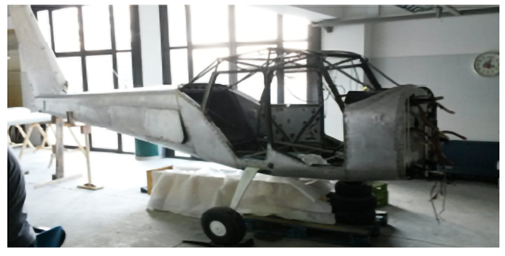
2. Technical Characteristics of the P64 OSCAR B Aircraft

At the Laboratory of Micromechanics and Materials for Aeronautical and Aerospace Technology of the Department of Civil, Energy, Environmental, and Material Engineering (DICEAM), Mediterranea University of Reggio Calabria (Italy) is located a P64 OSCAR aircraft under renovation (Figure 1), whose technical characteristics are detailed in

Table 1. Aircraft P64 OSCAR B: technical-data sheet.

Length	7.24 (m)	Wingspan	10 (m)
Weight	600 (kg)	Maximum take-off weight	1100 (kg)
Engine	Lycoming 0-360 180 (HP)	Cruise speed	250 (km/h)
Autonomy	4, 5 (h)	Maximum cruising altitude	5000 (m a.s.l.)

. Each wing of this aircraft is made up of two half-wings, each of which is connected to the fuselage by two pin-type connections and an upright connection. Each half-wing consists of a central body connected at the front to polyester resin and a glass fiber shell reproducing the front part of the wing profile. The used alloy is aluminum-copper 2024 characterized by good workability characteristics for machine tools, by high resistance and toughness, good resistance to atmospheric corrosion, and high resistance to high temperatures. The central body is made up of a front (main) side element and a “false” element (secondary) that make up the vertical walls. A series of ribs and cladding panels complete the structure. Flaps and ailerons are both made by a structure consisting of a single spar, ribs, and cladding panels, also in alloy 2024. Each half-wing houses a fuel tank; at the end of the main spar and of the false element are the plate attack wing–fuselages (see Figure 2a,c).

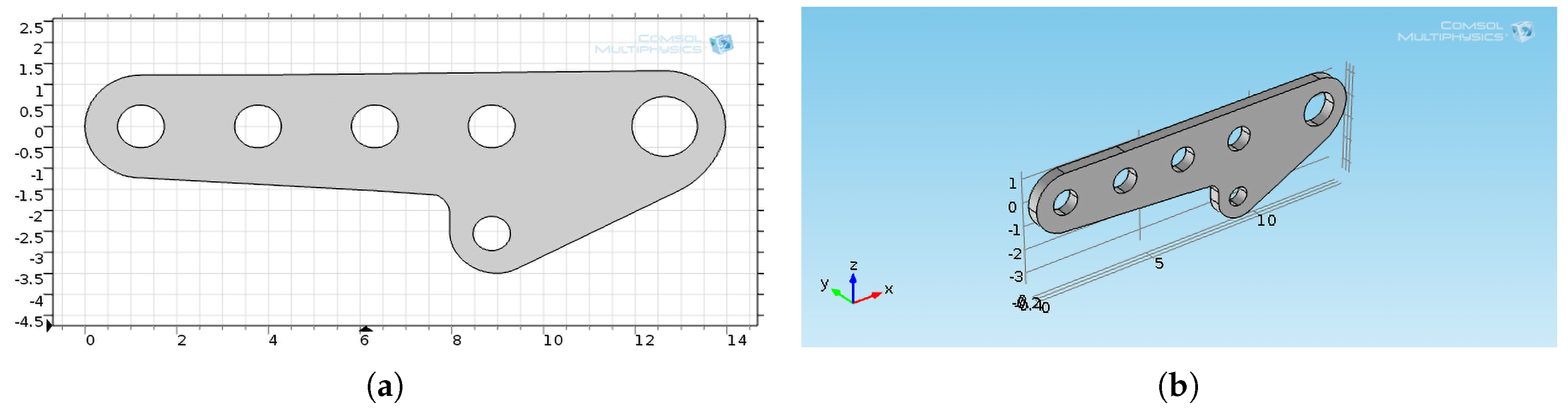
Plate-Attack Wing–Fuselage: Geometrical and Physical Characteristics

The plate is 14 cm long, has a thickness of $0.5$ (cm), and weighs $146.3$ (g). It also has four holes whose diameter is $0.7$ (cm) to accommodate the bolts for fixing to the main longitudinal element and a hole of $1.5$ (cm) in diameter to insert the pin for fixing to the fuselage (see Figure 2b,d). The used material was steel 3630N containing about $0.3\%$ C, about 1% Cr, and about 0.2% Mo, which give the material high mechanical properties suitable for aerospace applications. In it, there are also ions Mn and Si. Impurities due to S and P that are present with a lower percentage do not compromise the mechanical properties (the thermal and mechanical parameters of steel 3630N are listed in

Table 2. Steel 3630N: thermal–mechanical characteristics.

Symbol	Standard Values	Symbol	Standard Values
$c_p$	477 (J/(kg ${}^{\circ }$K))	k (thermal conductivity)	42.7 (W/(m ${}^{\circ }$K)
Thermal expansion coefficient	12.3 $\times {10}^{-6}$ (1/${}^{\circ }$K)	$\rho$ (density)	7850 (kg/mq)
Young’s module	200 $\times {10}^9$ (Pa)	Poisson’s coefficient	0.28 (dimensionless)

); unlike other alloys, it does not undergo alterations due to aging.

3. Proposed Model

3.1. Physical–Mathematical Modeling: Background

3.1.1. Heat Equation

The heat equation (or linear diffusion equation) for a function $T(\mathbf{v},t)$ (in our case, the absolute temperature), with $\mathbf{v}\in {\mathbb{R}}^n$ the spatial variable and $t>0$ the temporal variable, is a PDE taking the well known form [22,23,24]:

$$\frac{\partial T(\mathbf{v},t)}{\partial t}=D\Delta T(\mathbf{v},t)+f(\mathbf{v},t)$$

(1)

where D is a positive constant (diffusion coefficient), $\Delta$ is the Laplacian operator, and $f(\mathbf{v},t)$ is the external heat source. Equation (1) describes the evolution of $T(\mathbf{v},t)$ in a homogeneous and isotropic medium, with constant density $\rho$, receiving heat from a source. To achieve Equation (1), we indicate by r the rate of heat per unit of mass supplied to the body from the outside, and we consider a volume V. The energy-balance law requires that the rate of change in internal energy in V equal the flow of heat through $\partial V$ (frontier of V), due to conduction, plus the contribution due to the external source. If e is the internal energy per unit of mass (internal energy density), the total amount of internal energy in V is given by:

$${\int }_{V}e\rho dv.$$

(2)

Let us denote by $\mathbf{q}$ the heat-flux vector. Then, given an infinitesimal surface $d\sigma$ of the edge of V centered in $\mathbf{v}\in V$ with external unit vector $\mathbf{n}$, $\mathbf{q}·\mathbf{n}d\sigma$ expresses the amount of energy flowing through $d\sigma$. The scalar product is consistent with the observation that there is no flow of energy if vector $\mathbf{q}$ is normal to $\mathbf{n}$. The incoming heat flow through $\partial V$ is given by:

$$-{\int }_{\partial V}\mathbf{q}·\mathbf{n}d\sigma =-{\int }_V\nabla ·\mathbf{q}dv,$$

(3)

where we used the Gauss theorem. Finally, the contribution due to the external heat source is given by:

$${\int }_{V}r\rho dv.$$

(4)

The energy balance, therefore, requires the following relationship:

$$\frac{d}{dt}{\int }_{V}e\rho dv=-{\int }_V\nabla ·\mathbf{q}dv+{\int }_{V}r\rho dv.$$

(5)

3.1.2. Constitutive Laws

Let us now assume two constitutive relations. The first is Fourier’s law for heat conduction, according to which $\mathbf{q}$ is proportional to $T(\mathbf{v},t)$ as follows:

$$\mathbf{q}=-k\nabla T(\mathbf{v},t)$$

(6)

where thermal conductivity k is a constant positive related to the properties of the material [25]. Obviously, in some applications, k cannot be considered constant, but depends on T. The minus sign in Equation (6) is due to the fact that the heat flows from high temperature towards low temperature zones. The second constitutive equation links internal energy e and absolute temperature $T(\mathbf{v},t)$:

$$e=c_{p}T(\mathbf{v},t)$$

(7)

where $c_p$ is the specific heat at constant pressure of the material. Combining Equations (5)–(7) and taking into account that the Reynolds theorem is applicable, we obtain [19]:

$${\int }_V\left(c_p\rho \frac{\partial T(\mathbf{v},t)}{\partial t}-k\Delta T(\mathbf{v},t)-r\rho \right)dv=0.$$

(8)

from which, since Equation (8) is true for each V, then:

$$c_p\rho \frac{\partial T(\mathbf{v},t)}{\partial t}-k\Delta T(\mathbf{v},t)-r\rho =0.$$

(9)

We thus obtain Equation (1) in which $D=k/c_p\rho$ and $f=r/c_p$.

3.2. Initial and Boundary Conditions

To complete the formulation of the problem under study, we need to specify both initial and boundary conditions for Equation (1). In particular, regarding the initial conditions, we impose $T(\mathbf{v},0)$$\forall \mathbf{v}\in V$ in the plate at $t=0$. That is:

$$T(\mathbf{v},0)=g(\mathbf{v}).$$

(10)

Regarding the boundary conditions, it is possible to set the Dirichlet condition, specifying $\forall \mathbf{v}\in \partial V$:

$${T(\mathbf{v},t)|}_{\mathbf{v}\in \partial V}=T_q$$

(11)

in which $T_q$ is the external temperature. Alternatively, the Neumann boundary condition specifies flux of heat $\forall \mathbf{v}\in \partial V$ as follows:

$${k\nabla T(\mathbf{v},t)·\mathbf{n}|}_{\mathbf{v}\in \partial V}=q.$$

(12)

Finally, Newton’s law of cooling,

$${k\nabla T(\mathbf{v},t)·\mathbf{n}|}_{\mathbf{v}\in \partial V}=-hA(T(\mathbf{v},t)-T_q){|}_{\mathbf{v}\in \partial V},$$

(13)

can be exploited, in which h represents the heat-transfer coefficient. Condition (13) treats the heat flux through the surface, which depends on the temperature difference between the surface and environment. If radiant heat transfer between the body and the surrounding medium (or vice versa) becomes considerable, the following nonlinear condition:

$${k\nabla T(\mathbf{v},t)·\mathbf{n}|}_{\mathbf{v}\in \partial V}=-\sigma ϵA(T{(\mathbf{v},t)}^4-T_q^4){|}_{\mathbf{v}\in \partial V}$$

(14)

can be exploited. In this relation, $\sigma$ is the well known Stefan–Boltzmann constant, A is the surface, and $ϵ$ is surface emissivity, respectively [19].

Remark 1

(Parabolic frontier). No conditions were assigned at $t=t^{\ast }$, with $t^{\ast }$ the final time. The condition was only assigned on the so-called parabolic frontier ${\partial }_P{Q}_T$ of cylinder $Q_T$ given by the union of base $\overline{V}\times \{t=0\}$ and lateral part $S_T=\partial V\times (0,t^{\ast }]$:

$${\partial }_P{Q}_T=(\overline{V}\times \{t=0\})\cup S_T.$$

(15)

3.3. Steady-State Case

If T is independent of t (that is, $T(\mathbf{v})$), Equation (1) becomes Poisson’s equation:

$$\Delta T(\mathbf{v})=f(\mathbf{v});$$

(16)

otherwise, it takes the form of the Laplace equation:

$$\left\{\begin{array}{c}\Delta T(\mathbf{v})=0.\mathrm{in}V\hfill \\ T(\mathbf{v})=g=T_q\mathrm{on}\partial V.\hfill \end{array}\right.$$

(17)

Remark 2

(General formulation of the steady-state case). Equation (16) can be considered as a particular case of the following problem (in Dirichlet form):

$$\left\{\begin{array}{c}-\nabla ·(D\nabla T(\mathbf{v}))+\mathbf{b}·\nabla T(\mathbf{v})+{\sigma }_{1}T(\mathbf{v})=f(\mathbf{v})inV\hfill \\ T(\mathbf{v})=T_{q}on\partial V\hfill \end{array}\right.$$

(18)

where D, ${\sigma }_1$, f, and $\mathbf{b}$ are assigned functions (or constant). Generally, $D\in L^{\infty }(V)$, with $D(\mathbf{v})\ge D_0$, ${\sigma }_1\in L^2(V)$ with ${\sigma }_1(\mathbf{v})\ge 0$ almost everywhere in V, $\mathbf{b}\in {\left[L^{\infty }(V)\right]}^2$, with $\nabla ·\mathbf{b}\in L^2(V)$, and $f\in L^2(V)$. In these cases, the solution can give limit layers, that is regions next to $\partial V$ where the solution is characterized by strong gradients of T. Obviously, if both $\mathbf{b}·\nabla T(\mathbf{v})$ (convective term) and ${\sigma }_{1}T(\mathbf{v})$ (reactive term) are negligible, Problem (18) becomes Equation (16).

4. Preliminary Lemmas

As described above, both the Laplace Equation (17) and heat diffusion Equation (1) need suitable boundary conditions and initial-boundary conditions, respectively. However, for applicative reasons, it is imperative to ensure that $T(\mathbf{v})$ and $T(\mathbf{v},t)$ distributions, in both cases (steady-state and dynamical conditions), are uniquely determined to know the physical-mathematical conditions ensuring their existence and uniqueness. The following lemmas provide exhaustive indications about the existence and uniqueness of the solutions in both cases.

Lemma 1

(Laplace equation: maximum principle). If $T\in C(V)$ has the mean property in V (i.e., the value at the center of each sphere $B_R\subset \subset V$ equals the average of the values at the boundary $\partial B_R$) and ${\mathbf{v}}^{\ast }\in V$ is a global maximum or minimum point for T, then T is constant. In particular, if V is bounded and $T\in C(\overline{V})$ is not constant, then $\forall \mathbf{v}\in V$:

$$T(\mathbf{v})<\underset{\partial V}{max}TT(\mathbf{v})>\underset{\partial V}{min}T$$

(19)

Lemma 2

(Laplace equation: uniqueness, comparison, and stability for the Dirichlet problem). Let us suppose that $g\in C(\partial V)$. Then, the problem has, at most, a solution belonging to $C^2(V)\cup C(\overline{V})$. In addition, if $g_1\ge g_2$ on $\partial V$ and $g_1\ne g_2$ in at least one point on $\partial V$, then $T_{g_1}>T_{g_2}$ in V. Finally:

$$\underset{\overline{V}}{max}|T_{g_1}-T_{g_2}|=\underset{\partial V}{max}|g_1-g_2|.$$

(20)

Heat always flows towards regions where the temperature is lower. This has as the consequence that the solution of Equation (1) takes its global maximum and minimum values on ${\partial }_p{Q}_T$ (maximum/minimum principle). Moreover, $T(\mathbf{v},t)$ is independent of any changes in the data after t. Mathematically, we have the following lemma, which applies to continuous functions up to the edge of $Q_T$ with the temporal first derivative and spatial second derivatives continuous inside $Q_T$. Here, these functions are indicated by $C^{2,1}(Q_T)\cap C({\overline{Q}}_T)$ [19].

Lemma 3

(Heat equation: weak maximum principle). Consider $T(\mathbf{v},t)\in C^{2,1}(Q_T)\cap C({\overline{Q}}_T)$, such that:

$$\frac{\partial T(\mathbf{v},t)}{\partial t}-D\nabla T(\mathbf{v},t)=f(\mathbf{v},t)\le 0(resp.\ge 0)in{Q}_T.$$

(21)

Then, the maximum (resp. minimum) of T is on ${\partial }_P{Q}_T$:

$$\underset{{\overline{Q}}_T}{max}T(\mathbf{v},t)=\underset{{\partial }_P{Q}_T}{max}T(\mathbf{v},t)\left(resp.\underset{{\overline{Q}}_T}{min}T(\mathbf{v},t)=\underset{{\partial }_P{Q}_T}{min}T(\mathbf{v},t)\right).$$

(22)

In particular, if $T(\mathbf{v},t)$ is negative (positive) on ${\partial }_P{Q}_T$, then it is negative (positive) in ${\overline{Q}}_T$.

As a consequence of Lemma 3, we have that if:

$$\frac{\partial T(\mathbf{v},t)}{\partial t}-D\Delta T(\mathbf{v},t)=0in{Q}_T$$

(23)

the maximum and the minimum of T are located on ${\partial }_P{Q}_T$. In particular,

$$\underset{{\partial }_P{Q}_T}{min}T(\mathbf{v},t)\le T(\mathbf{v},t)\le \underset{{\partial }_P{Q}_T}{max}T(\mathbf{v},t)\forall (\mathbf{v},t)\in {\overline{Q}}_T.$$

(24)

Lemma 3 is a version of the weak maximum principle because it does not exclude the possibility that the maximum (minimum) can also be located on a point not belonging to ${\partial }_P{Q}_T$.

Lemma 4

(Heat equation: comparison, uniqueness, and stability for the Cauchy–Dirichlet problem). Let us consider $T_1(\mathbf{v},t)$ and $T_2(\mathbf{v},t)$ as solutions in $C^{2,1}(Q_T)\cap C({\overline{Q}}_T)$ of:

$$\frac{\partial T_1(\mathbf{v},t)}{\partial t}-D\Delta T_1(\mathbf{v},t)=f_1(\mathbf{v},t)$$

(25)

and:

$$\frac{\partial T_2(\mathbf{v},t)}{\partial t}-D\Delta T_2(\mathbf{v},t)=f_2(\mathbf{v},t)$$

(26)

respectively, with $f_1(\mathbf{v},t)$ and $f_2(\mathbf{v},t)$ bounded in $Q_T$. Then,

1. 

if $T_1(\mathbf{v},t)\ge T_2(\mathbf{v},t)$ on ${\partial }_P{Q}_T$ and $f_1(\mathbf{v},t)\ge f_2(\mathbf{v},t)$ in $Q_T$, then $T_1(\mathbf{v},t)\ge T_2(\mathbf{v},t)$ in $Q_T$;

2. 

the following estimation of stability holds:

$$\underset{{\overline{Q}}_T}{max}|T_1(\mathbf{v},t)-T_2(\mathbf{v},t)|\le \underset{{\partial }_P{Q}_T}{max}|T_1(\mathbf{v},t)-T_2(\mathbf{v},t)|+T\underset{{\overline{Q}}_T}{sup}|f_1(\mathbf{v},t)-f_2(\mathbf{v},t)|.$$

(27)

In particular, the Cauchy–Dirichlet problem admits a unique solution.

Lemma 5

(Het equation: strong maximum principle). Let us consider $T(\mathbf{v},t)\in C^{2,1}(Q_T)\cap C({\overline{Q}}_T)$ a sub-solution of Equation (1) (that is, $\frac{\partial T(\mathbf{v},t)}{\partial t}-D\Delta T(\mathbf{v},t)\le 0$). If $T(\mathbf{v},t)$ assumes the maximum value M on $({\mathbf{v}}_1,t_1)$ with ${\mathbf{v}}_1\in V$ and $0<t_1<t^{\ast }$, then $T(\mathbf{v},t)=M$ in $\overline{V}\times [0,t_1]$.

An analogous statement holds for the minimum if $T(\mathbf{v},t)$ is a super-solution (that is, $\frac{\partial T}{\partial t}-D\Delta T\ge 0$) in $Q_T$.

5. Model Realization in COMSOL-Multiphysics^®

5.1. Model Physics

By the heat-transfer module of COMSOL-Multiphysics^®, combined with the structural-mechanics module, we analyzed the thermal conduction on the plate attack wing–fuselage of a P64 OSCAR B aircraft. This is because these interfaces combine mechanical problems with problems due to thermal exchanges. This combination occurs when $T(\mathbf{v},t)$ acts as a thermal load for the mechanical interface, producing thermal expansion. As a first step, a steady-state condition was selected. After that, we studied the dynamical step.

5.2. Model Geometry

To perform the simulations, we first designed the steel plate in a 2D environment space of the COMSOL CAD interface, reproducing the geometry as shown in Figure 3a. Then, we implemented an extrusion, obtaining the final 3D model as depicted in Figure 3b.

5.3. Parameter Setting

This step required setting the mechanical and thermal parameters that are characteristic of the material constituting the steel plate as listed in Table 2.

5.4. Fixed-Constraint Setting

For our purposes, the fixed constraints of the plate on the main longitudinal component were selected through five holes, as shown in Figure 3b.

5.5. Plate Heat Transmission

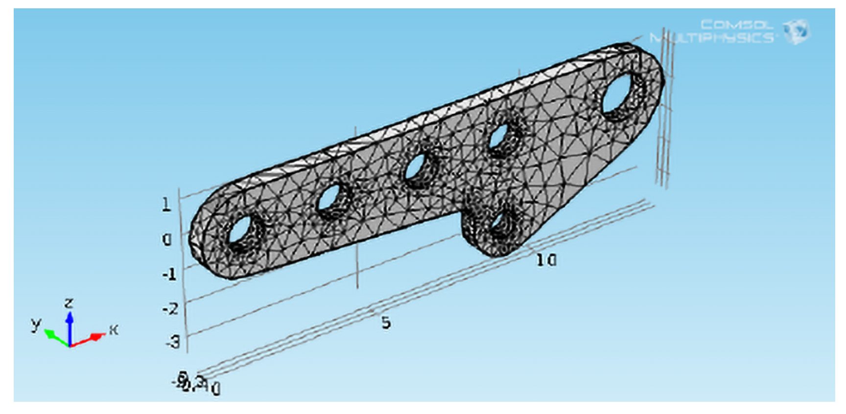
As is known, heat transmission occurs by conduction, convection, and radiation [26]. However, heat transmission does not exclusively occur in one of the three modes. Heat conduction is governed by Equation (1); Equation (13) governs convection mode; and finally, the Maxwell–Hertz–Plank equation describes the radiation mode [23,26]. However, for our purposes, we just considered heat transmission by conduction because the heat through convection and radiation, in our case, can be considered negligible [26].

5.6. Mesh Creation

First, the partition of the 3D domain was made by extending the selected faces of the geometry by extending a face on the adjacent face of a domain to partition it. Partitioning was used for the creation of tetrahedral meshes, subdividing the complex form domain (highly nonconvex) into a simpler mesh domain [23]. Furthermore, this could increase the level of parallelization (shared memory) during mesh generation. If the original geometry was meshed, unstructured tetrahedrons had to be used, which may not be the optimal choice. In order to achieve a more robust tetrahedral mesh and to avoid errors concerning failure to respect boundary-edge elements on the geometry face or internal errors in boundary respecting, we used a new algorithm involved in the “free tetrahedral” function in COMSOL MultiPhysics${}^{\circledR }$. In particular, the tessellation method was automatically set. First, the standard method was applied. If it failed, the new algorithm was used. However, in both cases, the Delaunay procedure was utilized [23]. In particular, the generation of the mesh was unstructured, so the triangulation was carried out in such a way that the sphere circumscribed to each tetrahedron did not contain vertices within it. This kind of triangulation was unique and maximized the minimum angle of the grid tetrahedra. However, to make the Delaunay procedure applicable to non-convex domains (such as of the plate at hand), we used the constrained Delaunay triangulation, which allowed fixing a set of sides of the mesh to be generated: the resulting grid necessarily associated these sides with some tetrahedron. In particular, we imposed the sides that defined the mesh boundary. It is worth pointing out that the constrained Delaunay triangulation is not a Delaunay triangulation because some of its tetrahedra may contain vertices belonging to the initial set. However, the vertices were only and exclusively the original ones specified in the set, and no others were added [23]. Finally, we obtained a mesh consisting of 3623 volume elements, 2208 surface elements, and 407 edge elements (see Figure 4).

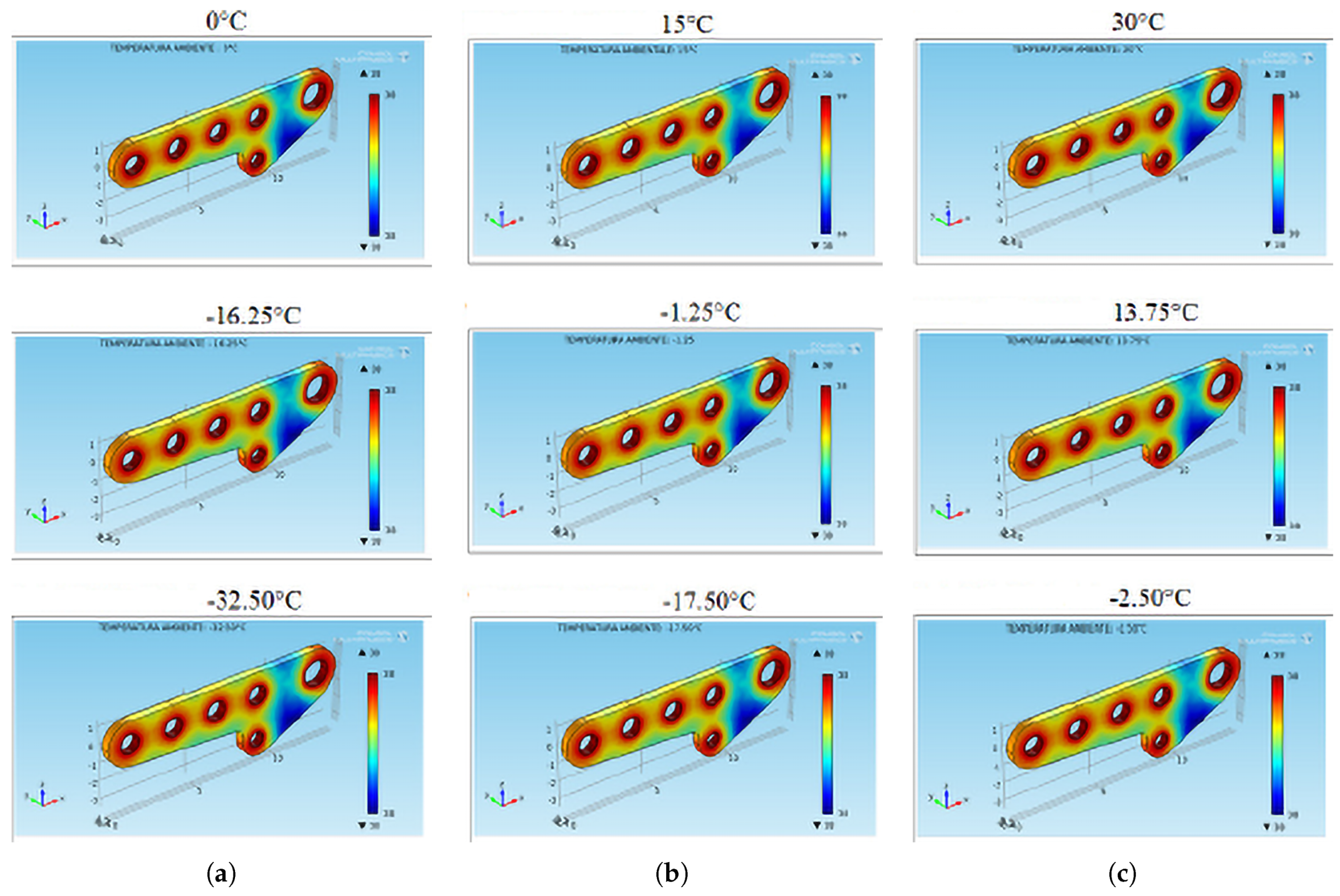
5.7. Choice of Significant Temperatures

Once the geometry of the plate was implemented and the problem was set from a physical–mathematical point of view, it was necessary to choose significant external temperatures to take into account the most important phases of a flight. This link derived from the fact that $T_q$ (external temperature), starting from sea level, almost linearly decreases by 3.25 (${}^{\circ }$C) for each 500 (m) of altitude, up to $11.000$ (m) (36,089 (ft)), beyond which and up to 22,000 (m) (82,021 (ft)), it remains constant at the value of −56.5 (${}^{\circ }$C). We therefore chose to simulate the behavior of the plate at sea level and 2500 and 5000 (m) corresponding to 0, 15, and 35 (${}^{\circ }$C), respectively, taking into account that a P64 OSCAR B in safe conditions can reach a maximum altitude of 5000 (m) (for details, see

Table 3. Significant temperatures depending on flight altitude.

${\mathit{T}}_{\mathit{q}}$ (°C)	Flight Altitude (m)	${\mathit{T}}_{\mathit{q}}$ (°C)	Flight Altitude (m)	${\mathit{T}}_{\mathit{q}}$ (°C)	Flight Altitude (m)
$\mathbf{0}$	$\mathbf{0}$	$\mathbf{15.00}$	$\mathbf{0}$	$\mathbf{35.00}$	$\mathbf{0}$
−3.25	500	11.75	500	31.75	500
−6.50	1000	8.50	1000	28.50	1000
−9.75	1500	5.25	1500	25.25	1500
−13.00	2000	2.00	2000	22.00	2000
$-\mathbf{16.25}$	$\mathbf{2500}$	$-\mathbf{1.25}$	$\mathbf{2500}$	$\mathbf{18.75}$	$\mathbf{2500}$
−19.50	3000	−4.50	3000	15.50	3000
−22.75	3500	−775	3500	12.25	3500
−26.00	4000	−11.00	4000	9.00	4000
−29.25	4500	−14.25	4500	5.75	4500
$-\mathbf{32.50}$	$\mathbf{5000}$	$-\mathbf{17.50}$	$\mathbf{5000}$	$\mathbf{2.50}$	$\mathbf{5000}$

).

5.8. Boundary-Condition Setting

In this work, we used temperature $T(\mathbf{v})=T_q$ on $\partial V$ (Dirichlet’s condition (11)) as a boundary condition. However, COMSOL-Multiphysics^® requires, by default, the computation of heat-transfer coefficient values h related to significant temperatures depending on flight altitudes as specified in the following subsection.

5.9. Determination of Heat-Transfer Coefficients h

To determine h, we combined Equations (12) and (13), obtaining [26,27]:

$$h=\frac{q}{A(T_q-T_s)}$$

(28)

in which q represents the exchanged heat flow (Watt), A is the area of the heat-exchange surface (m${}^2$), and $T_q-T_s$ is the difference of temperature (${}^{\circ }$K). Moreover, combining Equations (12) and (14), we obtain:

$$q=ϵA\sigma (T_q^4-T_s^4)$$

(29)

so that Equation (28), considering Equation (29), becomes:

$$h=\frac{ϵA\sigma (T_q^4-T_s^4)}{A(T_q-T_s)}=ϵ\sigma (T_q+T_s)(T_q^2+T_s^2)$$

(30)

where $ϵ=0.07$ is the emissivity of polished steel, $\sigma$ is the Stefan–Boltzmann constant (W/m${}^2$${}^{\circ }$K${}^4$), and $T_q$ and $T_s$ are the room and the plate temperatures, respectively. Setting $ϵ=0.07$, $T_s{=311.15(}^{\circ }$K) (polished steel), $\sigma =5.67\times {10}^{-8}($ W/m${}^2$${}^{\circ }$K), we obtained the required values of h related to significant temperatures depending on flight altitudes (see

Table 4. h values for significant temperatures depending on flight altitude.

${\mathit{T}}_{\mathit{q}}$$({}^{\circ }\mathbf{C})$	h$\left(\frac{\mathbf{Watt}}{{\mathbf{m}}^2\mathbf{K}}\right)$	${\mathit{T}}_{\mathit{q}}$$({}^{\circ }\mathbf{C})$	h$\left(\frac{\mathbf{Watt}}{{\mathbf{m}}^2\mathbf{K}}\right)$	${\mathit{T}}_{\mathit{q}}$$({}^{\circ }\mathbf{C})$	h$\left(\frac{\mathbf{Watt}}{{\mathbf{m}}^2\mathbf{K}}\right)$
0	0.3671	15	0.4235	35	0.4482
−16.25	0.3681	−1.25	0.3631	13.75	0.4269
−32.5	0.3371	−17.50	0.3658	−2.5	0.3628

).

6. Relevant Results

6.1. Simulations in Steady-State Conditions

As above specified, heat transfer in the plate in this work was assumed to be by conduction so that Equation (1) could be selected in COMSOL MultiPhysics${}^{\circledR }$ in its steady-state version ($\partial T(\mathbf{v})/\partial t=0$). Moreover, since the external heat source was null,

$$\left\{\begin{array}{c}\Delta T(\mathbf{v})=0\mathrm{in}V\hfill \\ T(\mathbf{v})=g=T_q\mathrm{on}\partial V.\hfill \end{array}\right.$$

(31)

in which $T_q$ represents the temperature to which the plate is subjected during each simulation. As is known, Problem (31) can be considered as a particular case of the general Problem (18) (in Dirichlet form) in which the reactive term is neglected and $\mathbf{b}·\nabla T(\mathbf{v})=0$ because $\mathbf{b}$ represents a velocity that, in steady-state conditions, vanishes. Then, Problem (18) becomes:

$$\left\{\begin{array}{c}\nabla ·(D\nabla T(\mathbf{v}))=0\mathrm{in}V\hfill \\ T(\mathbf{v})=g=T_q\mathrm{on}\partial V.\hfill \end{array}\right.$$

(32)

If D is considered as a constant, then Problems (31) and (32) coincide. Then, a set of simulations in steady-state conditions was performed. Figure 5a–c depicts the 3D simulations subjecting the plate to different $T_q$ values. In particular, in Figure 5a, $T_q=0$ (°C) at sea level, $T_q=-16.25$ (°C) if the flight altitude is 2500 (m), and $T_q=-32.50$ (°C) when the flight altitude is 5000 (m) (see Table 3). Analogously, in Figure 5b, $T_q=15$ (°C) at sea level, $T_q=-1.25$ (°C) when the flight altitude is 2500 (m), and $T_q=-17.50$ (°C) when the flight altitude is 5000 (m). Finally, in Figure 5c, $T_q=30$ (°C) at sea level, $T_q=13.75$ (°C) when the flight altitude is 2500 (m), and $T_q=-2.50$ (°C) when the flight altitude is 5000 (m). The simulations of the thermal maps were obtained with an uneven color over the entire surface, but they are clearly distinguishable from the more and less intense areas. Red highlights the critical zones due to both the plate geometry and the type of material used. In contrast, blue shows plate areas that are poorly affected by thermal stress.

Remark 3

(On the existence and uniqueness of thermal maps in steady-state conditions). It is worth noting that the fundamental solution of Problem (31) is [19]:

$$T(\mathbf{v})=\frac{1}{{n(n-2)\alpha (n)|\mathbf{v}|}^{n-2}}n\ge 3$$

(33)

where n is the dimension of the space and $\alpha (n)$ is the volume of the ball of unit radius, so that, for $n=3$, it makes sense to write:

$$T(\mathbf{v})=\frac{1}{4\pi |\mathbf{v}|}.$$

(34)

Then, $\forall \mathbf{v}\in V$, the solution $T(\mathbf{v})$ exists. In fact, in the steady-state simulations, $\mathbf{v}\ne 0$, so that $T(\mathbf{v})$ is physically bounded. In addition, fixing a values for $T_q$, Lemma 2 guarantees the uniqueness for $T(\mathbf{v})$, ensuring that the thermal maps in each simulation are unique when $T_q$ is fixed.

Remark 4

(On functional space for $T(\mathbf{v})$). By this set of simulations, it can be seen that the most critical areas concerned the portion of $\partial V$ next to the holes where thermal stresses were strongly present. This was congruent with the fact that solution T provided limit layers next to $\partial V$ characterized by a strong gradient of T (see Remark 2). It was also congruent with Lemmas 3 and 5. Experimentally, $T(\mathbf{v})\in C^{2,1}(Q_T)\cap C({\overline{Q}}_T)$ because both the thermal and mechanical properties of the steel used constituting the plate admit continuous-time variation of the temperature and very reduced but continuous changes of its second spatial derivatives in $Q_T$.

Remark 5

(On the location of the minimum and maximum values of thermal stress on the plate). Consider that $\partial T/\partial t=0$, $f(\mathbf{v})=0$, and $\Delta T=0$, as highlighted in Equation (21). Then, maximum T values took place on $\partial V$ (zones around the holes). On the other hand, far from the holes, thermal stresses were very low. In particular, in some portions of $\partial V$ far from the holes, the thermal stress assumed minimum values (see Equation (21)). This was again congruent with Lemmas 3 and 5 because the maximum and minimum values were located on $\partial V$. To confirm this experimentally, we chose two generic points of the plate far from the holes, whose vectors’ positions were ${\mathbf{v}}_1$ and ${\mathbf{v}}_2$, respectively. It follows that ${\mathbf{v}}_1-{\mathbf{v}}_2$ was sufficiently high (because they were internal to the connected portions of V), so that $T({\mathbf{v}}_1-{\mathbf{v}}_2)$ resulted in being greatly attenuated. Equation (34) results:

$$T({\mathbf{v}}_1-{\mathbf{v}}_2)=\frac{1}{4\pi |{\mathbf{v}}_1-{\mathbf{v}}_2|}$$

(35)

then in the area of the plate far from the holes, the temperature was not high. On the other hand, near the holes of the plate, there was an increase of temperature, as can be also noticed by the results reported in Figure 5 (to reproduce as much as possible the edge of the holes, it was necessary to consider small values of $|{\mathbf{v}}_1-{\mathbf{v}}_2|$).

The same considerations described in Remarks 4 and 5 are still valid for the depicted simulations in Figure 5b,c. Although these simulations were in steady-state conditions, they could be considered as a good model giving interesting information about more thermally stressed holes (and consequently, from those mechanically stressed). To give further information about the evolution of the thermal-stress distribution required by both designers and technicians, we needed to develop dynamical simulations when thermal shock was applied. These simulations could be used as a prediction model of $T(\mathbf{v})$ to also provide designers with useful and indispensable support for the optimization of the plate geometry/material or to help technicians with deciding if the plate can be reused after a sequence of flights.

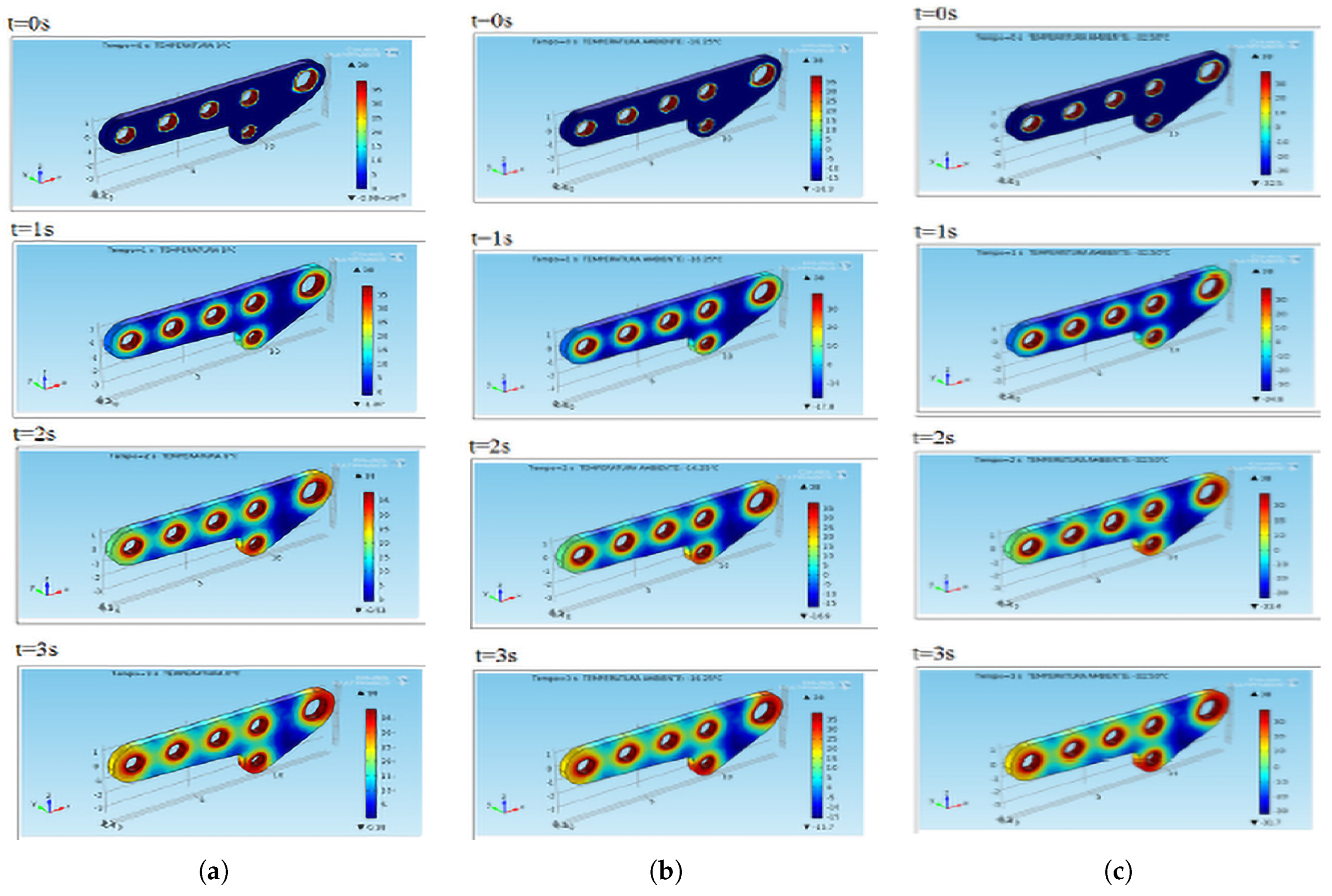
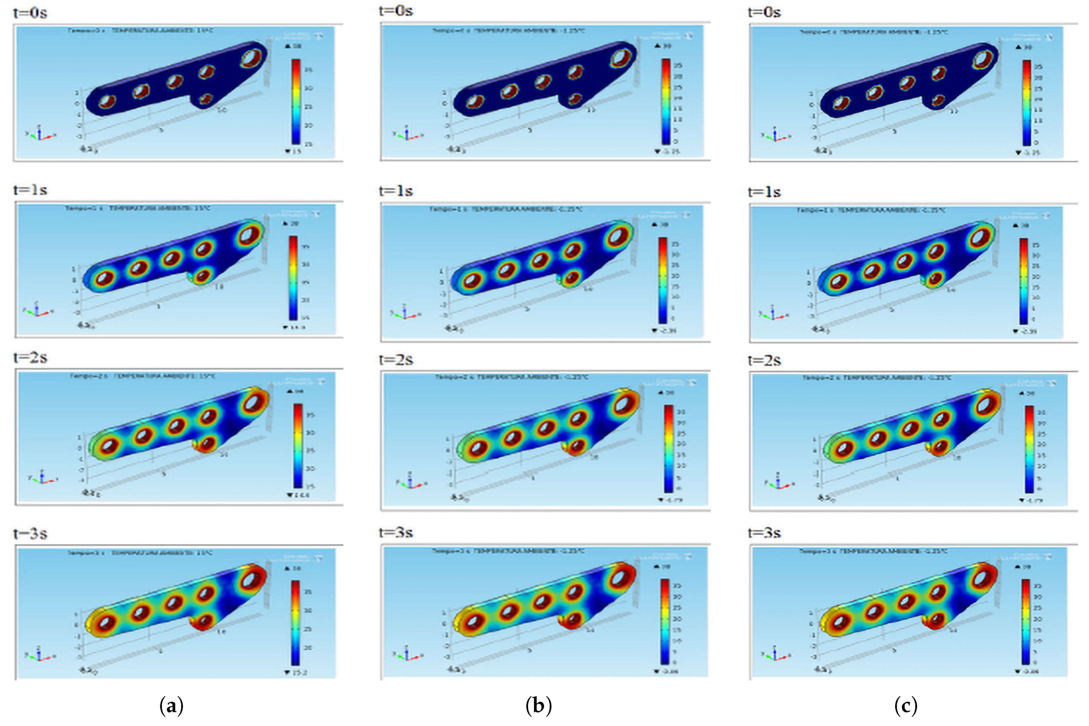
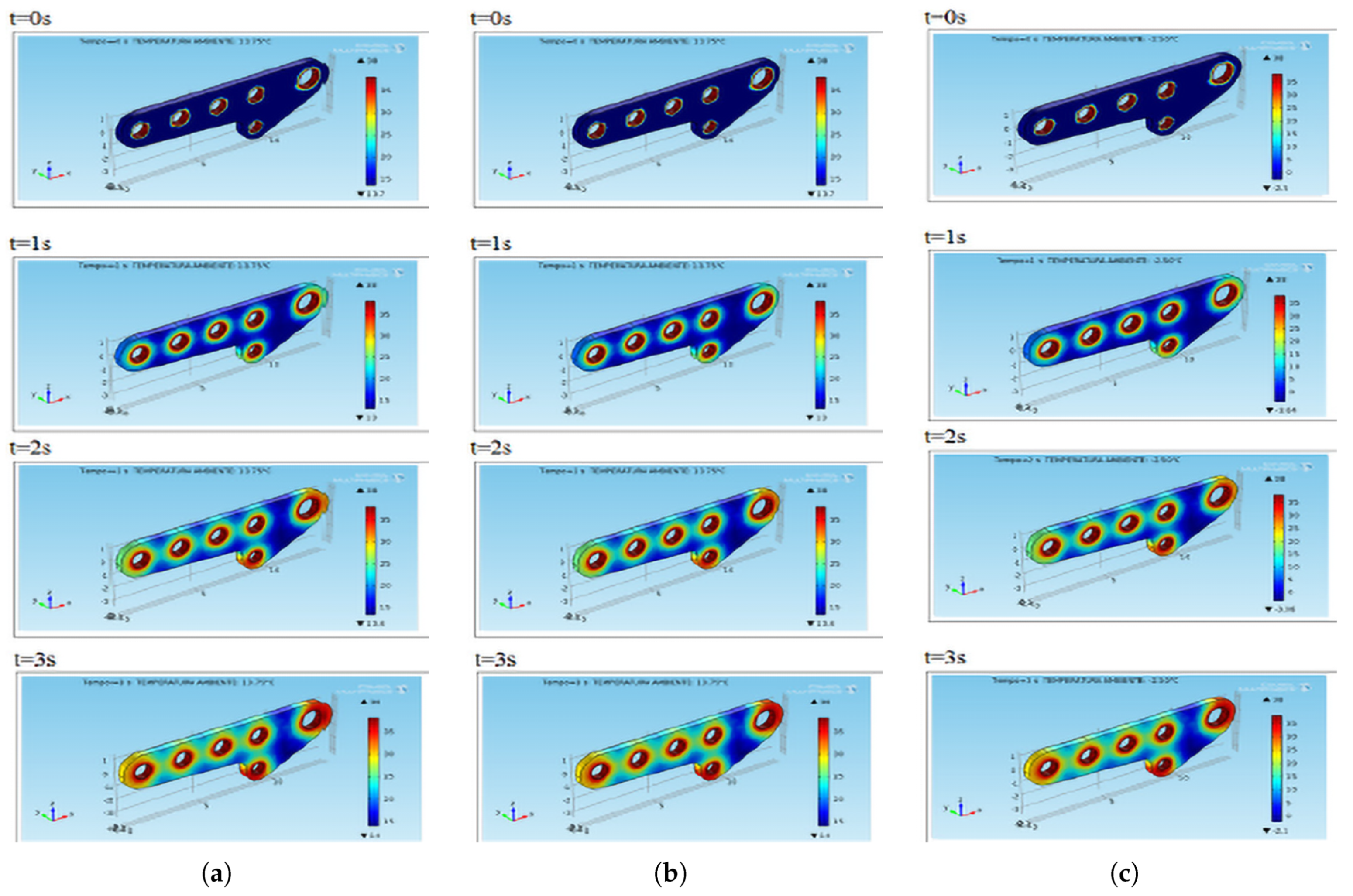
6.2. Simulations in Dynamic Conditions

Our problem in dynamic conditions can be written as follows:

$$\left\{\begin{array}{c}\frac{\partial T(\mathbf{v},t)}{\partial t}-D\Delta T(\mathbf{v},t)=0\hfill \\ T(\mathbf{v},0)=g(\mathbf{v})=T_q\hfill \\ {T(\mathbf{v},t)|}_{\mathbf{v}\in \partial V}=T_q\hfill \end{array}\right.$$

(36)

in which the initial condition is $T(\mathbf{v},0)=g(\mathbf{v})=T_q$ and the boundary condition is ${T(\mathbf{v},t)|}_{\mathbf{v}\in \partial V}=T_q$. Equation (36) and related initial and boundary conditions were implemented in COMSOL MultiPhysics${}^{\circledR }$ in order to obtain a set of thermal maps in dynamical conditions.

Remark 6

(On the existence and uniqueness of thermal maps in dynamical conditions). As is known, the fundamental solution of Problem (36) can be written as follows:

$$\left\{\begin{array}{c}{\Gamma }_D(\mathbf{v},t)=\frac{Q}{{(\sqrt{4\pi Dt})}^3}{e}^{-\frac{{|\mathbf{v}|}^2}{4Dt}}\hfill \\ Q={\int }_{{\mathbb{R}}^3}T(\mathbf{v},t)d\mathbf{v}\hfill \end{array}\right.$$

(37)

which represents a curve very close to a Gaussian one. It can be observed that whatever $\mathbf{v}$ in the plate, the solution exists because ${\Gamma }_D$ is bounded. Furthermore, Lemma 4 guarantees the uniqueness for $T(\mathbf{v},t)$ ensuring that the thermal maps in each dynamical simulation are unique when both initial and boundary conditions are fixed.

Remark 7

(On the functional space for $T(\mathbf{v},t)$). Even in dynamic simulations, the same considerations apply as in Remark 4.

Remark 8

(On the location of the minimum and maximum values of thermal stress on the plate). As in the previous steady-state simulations and far from the holes of the plates, the thermal stress assumed low values also in dynamical simulations. In fact, considering ${\mathbf{v}}_1$ and ${\mathbf{v}}_2$ two different position vectors and for a fixed $t=t^{\ast }$, Equation (37) can be written as follows:

$${\Gamma }_D({\mathbf{v}}_1-{\mathbf{v}}_2,t)=\frac{Q}{{(\sqrt{4\pi D{t}^{\ast }})}^3}{e}^{-\frac{|{\mathbf{v}}_1-{\mathbf{v}}_2{|}^2}{4D{t}^{\ast }}}.$$

(38)

If ${\mathbf{v}}_1$ and ${\mathbf{v}}_2$ lie in the areas far from the holes of the plates, ${\Gamma }_D({\mathbf{v}}_1-{\mathbf{v}}_2,t)$ assumes low values. In other words, in dynamical conditions and far from the holes, the thermal stresses were low. The contrary happened next to the holes: here, the temperature increased considerably, as well as the thermal stress (to reproduce as much as possible the contour of each hole, it was imperative to consider small values of $|{\mathbf{v}}_1-{\mathbf{v}}_2|$).

To understand how thermal stresses evolve in time t in the plate when thermal shock $T_q$ is initially applied, we needed to perform a set of simulations that focused on thermal-stress distributions in the plate for $t\in [0,+\infty )$ (s). In particular, we focused on the evolution of the thermal-stress distribution for $t\in \{0,1,2,3\}$ (s), with $\Delta t=1$ s, because it represented a more dangerous time interval for the plate after the application of a thermal shock. In fact, in the plate after 3 s, T started to decrease, so that the more dangerous time interval was $[0,3]$ s [26].

Remark 9

(On the choice of the dangerous time interval for the plate after the application of a thermal shock). After having fixed a vector position $\mathbf{v}$ (in other words, after having chosen a particular point on the surface of the plate), the fundamental solution (37) can be written as ${\Gamma }_D(t)$. For each t, this was a bell shaped definite positive function such that ${\Gamma }_D(t)\to 0$ as the time $t\to 0$ and ${\Gamma }_D(t)\to 0$ as the time $t\to +\infty$. Then, setting $\mathbf{v}$ and varying the time t, the temperature increased, reaching the stationary point (at the time $t^{\ast }$), and finally decreased, as highlighted in the simulations. For each simulation, $t=t^{\ast }=3$ s, so that $\left[03\right]$ s represented the dangerous time interval for the plate after the application of the thermal shock.

For dynamic simulations, we also used the physics and geometry of the model, the setting of the parameters and continuum mechanics, and also the mesh creation related to the steady-state simulation as detailed in Section 5.1, Section 5.2, Section 5.3, Section 5.4, Section 5.5 and Section 5.6, respectively. Moreover, for analysis uniformity, we chose the same significant temperatures here as those described in Section 5.7. The simulations produced Figure 6a–c, Figure 7a–c and Figure 8a–c. In particular, Figure 6a–c shows the performance in dynamic conditions with initial thermal shock $T_q=0{}^{\circ }$C (sea level), $-16.25{}^{\circ }$C (2500 (m)), and $-32.5{}^{\circ }$C (5000 (m)), respectively. It is easy to argue that after 3 (s) of the application of $T_q$, the plate presented the critical areas strongly highlighted in red. Moreover, in blue, the areas less thermally loaded were evidenced. As for the steady-state simulations, the same consideration discussed in Remarks 4 and 5 were still valid. The obtained results notably did not depend on the use of other parameters such as atmospheric pressure and wing weight, which weighed even more on the areas highlighted in red. The discussion can be easily extended to the other simulations whose performance is depicted in Figure 7a–c and Figure 8a–c.

To validate the performance of the results achieved by the implementation of the parabolic model in COMSOL MultiPhysics${}^{\circledR }$, we compared the obtained results with those achieved by an experimental investigation by IR thermal imaging.

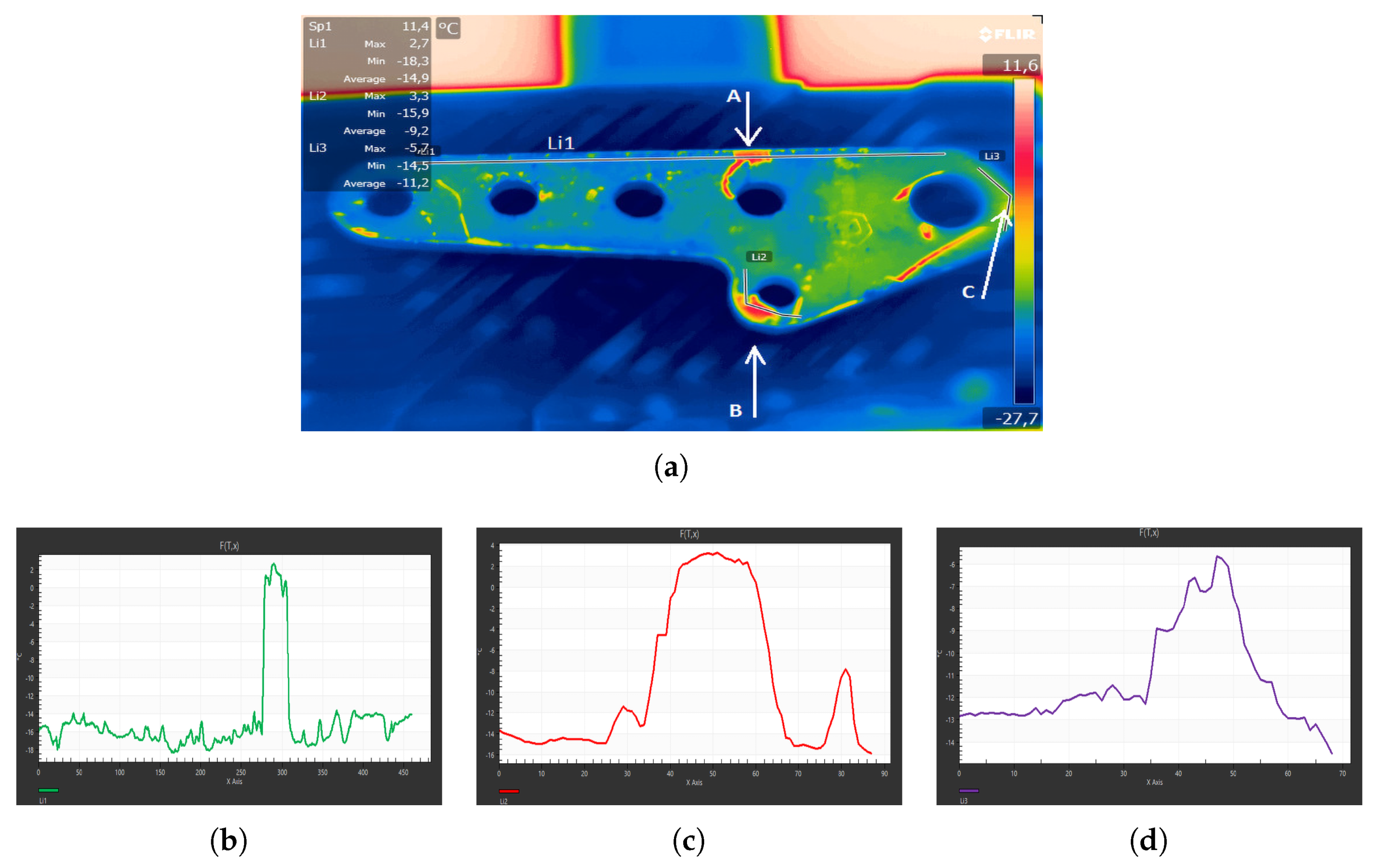
7. Experimental Investigations by IR Thermal Imaging and Result Comparison

7.1. Pretreatment with Penetrating Liquids

The plate was pretreated with penetrating liquids to verify the absence of defects (the presence of at least one defect obliges that the plate not be reused). Particularly, its surface was cleaned with a degreasing agent and heated to $35$ (°C), then coated with a fluorescent penetrating liquid. The excedent fluid was removed with a hydrophilic emulsifier. After washing, the penetrating liquid left inside the defects rose to the surface and left a signal with a much larger size than the defect in the detector. The surface was analyzed with a UV radiation lamp that guaranteed high contrast with high detection sensitivity [13]. Analysis did not show any type of defect in the plate, so it made sense to perform a survey for the detection of thermal stresses.

7.2. IR Thermography: Brief Overview

This is an NDT measurement of the IR radiation emitted by a body to determine its surface temperature. IR radiation is located between the visible spectrum and radio frequencies/microwaves with a wavelength between 1 (mm) and 0.7 $\mathsf{\mu }$(m) (frequencies between $3\times {10}^{11}$ and $4\times {10}^{14}$ (Hz)). Even if the human eye cannot see it, its presence is perceived by the thermal effect it produces. IR thermography visualizes and quantifies thermal flows through the generation of maps (thermograms) that associate a color with a detected temperature to evaluate the condition of materials. It is necessary to know (or to hypothesize) the distribution of surface temperatures in the absence of defects to compare them with the actual distribution measured during a test. An anomaly in temperature distribution indicates a possible defect, visible by a color spot. In this work, we used a FLIR SC660 camera with a resolution of $640\times 480$ and a wavelength between 0.7 and 1 (D m). The achieved images (thermograms) were processed by FLIR RESEARCH IR software. After appropriate calibration of the camera, three types of simulations were conducted: at below-zero temperature ($-18{(}^{\circ }$C)), at room temperature ($15{(}^{\circ }$C)), and at about $30{(}^{\circ }$C). These temperatures were slightly different from the significant temperatures of $-16.25{(}^{\circ }$C), $-15{(}^{\circ }$C), and $35{(}^{\circ }$C) as shown in Table 3. This was due to technical laboratory requirements.

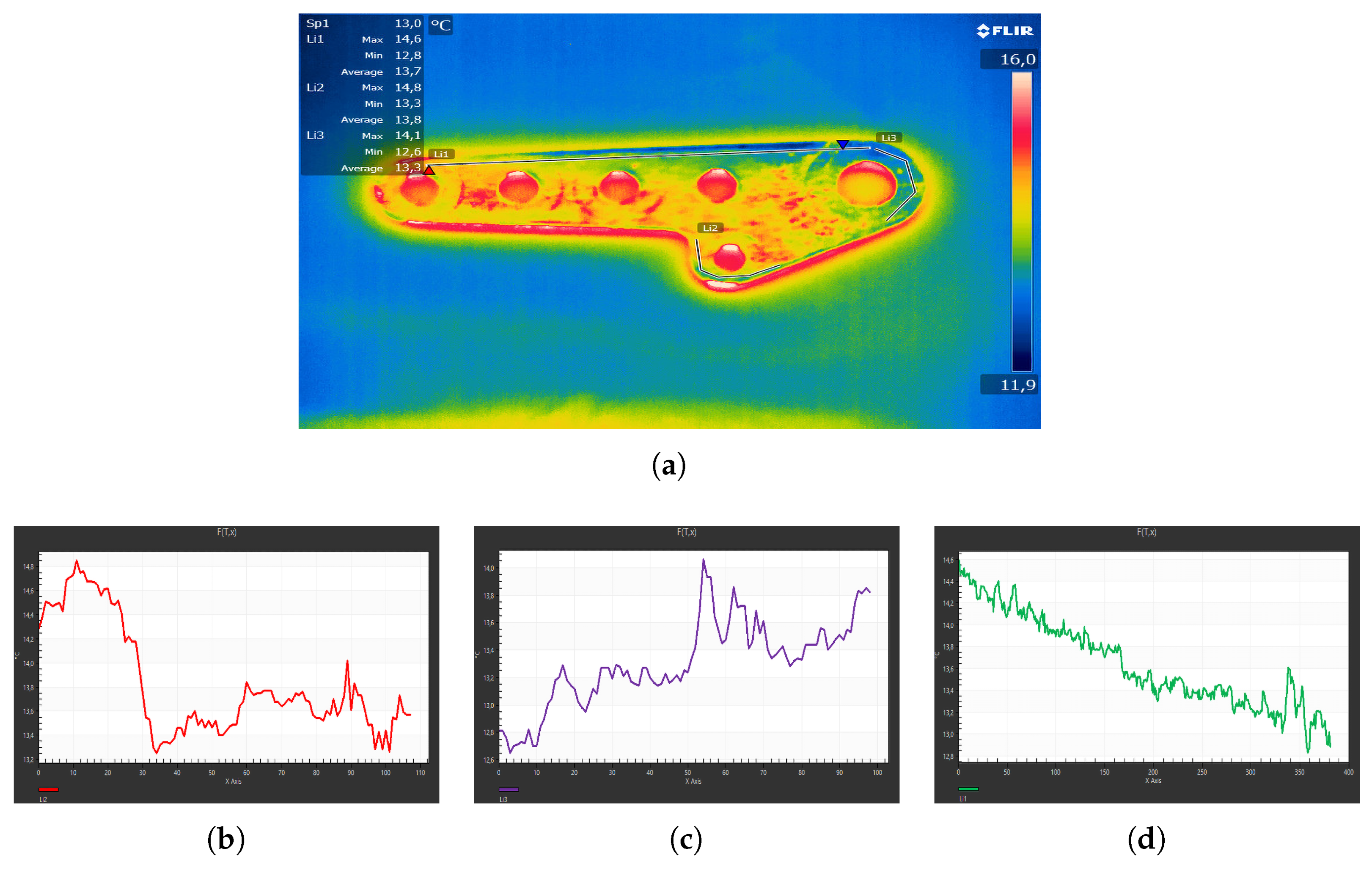
7.3. Thermographic Investigation at −18 (°C)

The plate was placed in the freezer for 15 min to reach $-18{(}^{\circ }$C). The achieved thermogram (Figure 9a) shows three critical areas identified by A, B, and C. Using the marker Li1 (shown in Figure 9a in the area identified by A), we obtained the trend of the temperature (see Figure 9b). Figure 9c depicts the trend of temperature identified by the marker Li2 (see Figure 9a) in the area identified by B) in which a sudden change in temperature was detected, but in a wider space with respect to the area A. Finally, Figure 9d shows a clear change in temperature near the point C. Comparing this result with the performance achieved by COMSOL MultiPhysics${}^{\circledR }$, it is evident that the critical areas identified in the simulation corresponded exactly to those highlighted with the thermographic analysis.

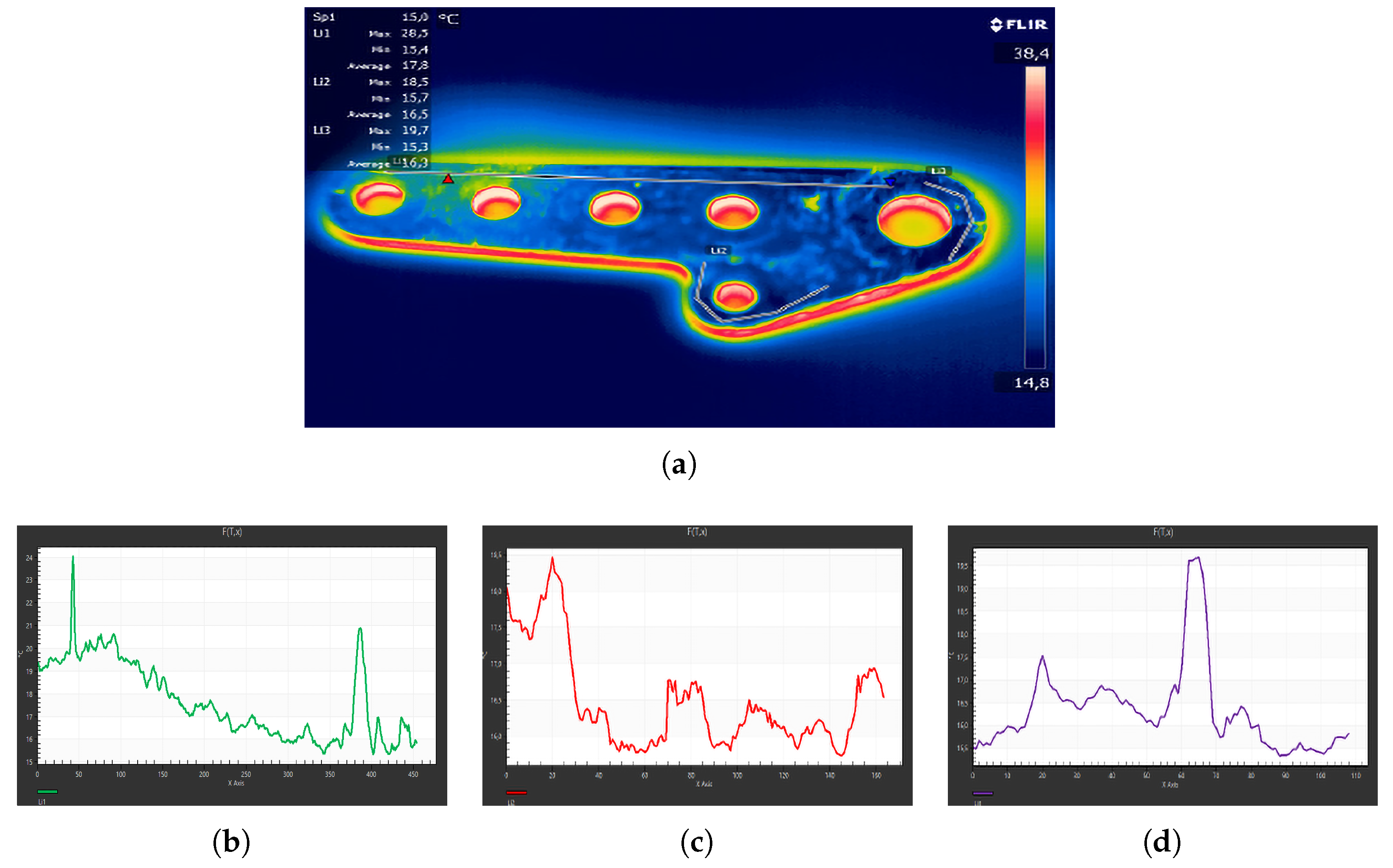
7.4. Thermographic Investigation at 15 (°C)

As in Section 7.3, the procedure was performed at $15$ (°C), obtaining the thermogram shown in Figure 10a. Through analysis, we deduced that the temperature along its upper area (marker Li1 in Figure 10a) showed an erratic trend (Figure 10b) with evident thermal jumps. Analysis along the lower side (Figure 10c) showed the existence of a series of sudden temperature changes confined in limited areas. Even near the holes (Figure 10d), we noted critical areas. Comparing the experiment performance with the simulated performance at $15$ (°C), one could see critical areas, common to the two models, concentrated mainly near the holes.

7.5. Thermographic Investigation at 30 (°C)

With a heat gun, the plate was heated to up to $30$ (°C), obtaining the thermogram shown in Figure 11a. Analysis of the thermogram highlighted the existence of two sudden temperature changes (see Figure 11b), identifying two critical areas. Figure 11c,d highlights the presence of areas that need to be more carefully analyzed. In this case, the overlapping of the critical areas obtained in the simulation phase and in the experiment tests was also evident.

8. Conclusions and Perspectives

In this work, the authors presented a second-order parabolic model implemented in COMSOL Multiphysics${}^{\circledR }$ to analyze thermal stresses (distribution of temperature T) in a plate attack wing–fuselage of a P64 OSCAR B aircraft. Starting from the details of the technical characteristics of the aircraft, the proposed model was mathematically detailed in terms of equations and boundary and initial conditions. In addition, important well known results of the existence/uniqueness and localization of minimum/maximum T values for both steady-state and dynamical conditions, respectively, were presented. Then, the authors detailed the model realization in COMSOL MultiPhysics${}^{\circledR }$, modeling both the physics and geometry of the problem and then setting the parameter and constraints. The 3D mesh was created by an innovative technique exploiting the constrained Delaunay triangulation suitable for the plate under study (non-convex domain).

Once the authors chose significant temperatures of aeronautical interest, they performed a set of simulations in steady-state conditions at different flight altitudes. The simulated results put in evidence critical areas of the plate where the thermal stress appeared significant. This fact was also demonstrated exploiting the fundamental solution for the heat equation in steady-state conditions (Laplace equation), highlighting the minimum and maximum values of the temperature on the plate.

The results also highlighted the model’s capability to evaluate the presence and exact position of any critical points (in the steady-state case), also showing the T distribution evolution in time on the plate (in dynamical conditions), putting into evidence and quantifying a dangerous time interval for the plate after the application of a thermal shock. Moreover, in the dynamic conditions, the location of the minimum and maximum values of the thermal stress on the plate were proven by exploiting the fundamental solution of the heat equation. Finally, the validity of the model was confirmed via comparison with the obtained results by IR thermographic analysis. In particular, the results achieved by the proposed model in terms of critical areas of thermal stress on the plate were totally comparable (both in position and intensity) with the results achieved by IR thermographic analysis. The proposed model presented here was a reliable prediction system of critical plate areas, helping technicians to establish if the plate can be reused. Moreover, the dynamic approach fixed the number of flights beyond which the plate could not be reused. The competitiveness of this model lied in the quality and quantity of information that could be extracted from the simulations, making it possible to identify the geometric characteristics of critical areas both in terms of shape and size. However, despite the good agreement between numerical simulations and thermographic images, the proposed model resulted in not being well suitable for real-time applications due to the related heavy computational burden. Anyway, taking advantage of the fact that the transition between low thermal loads and high thermal loads is not crisp, but gradual, it would be worthwhile to model the problem using soft computing techniques. In particular, fuzzy computation techniques could be exploited to create a system handled by a bank of IF-THEN fuzzy rules easily readable by non-experts and, in any case, updatable by the knowledge of an expert. Finally, the reduced computational load of these systems should allow obtaining low cost hardware implementation. This will be the scope of a future work.

References

1. Yillikci, Y.K.; Findik, F. Survey of Aircraft Materials: Design for Airworthiness and Sustainability. Period. Eng. Nat. Sci. 2013, 1, 8–33. [Google Scholar]
2. Fleischer, R.L. High-Strength, High-Temperature Intermetallic Compounds. J. Mater. Sci. 1987, 22, 2281–2288. [Google Scholar] [CrossRef]
3. Gladkov, O. To the theory of internal thermal equilibrium in heterogeneous structures. Tech. Phys. Lett. 1998, 24, 29–36. [Google Scholar] [CrossRef]
4. Gladkov, O. On the theory of nonlinear thermal conductivity. Tech. Phys. Lett. 2016, 61, 157–164. [Google Scholar] [CrossRef]
5. Kumar, A.; Sharma, K.; Dixit, A.R. A Review of the Mechanical and Thermal Properties of Graphene and ints Hybrid Polymer Nanocomposites for Strctural Applications. J. Mater. Sci. 2018, 54, 5992–6026. [Google Scholar] [CrossRef]
6. Axtman, S.J.; Wilck, J.H. A Review of Aviation Manufacturing and Supply Chain Processes. Int. J. Supply Chain Manag. 2007, 4, 22–27. [Google Scholar]
7. Villa dos Santos, C.; Leiva, D.R.; Rodrigues Costa, F.; Rodrigues Gregolin, J.A. Materials Selection for Sustainable Executive Aircraft Interiors. Mater. Res. 2016, 19, 339–352. [Google Scholar] [CrossRef]
8. Smurov, M.Y.; Gubenki, A.V.; Ksenofontova, T.Y.; Staroselets, V.S. Comparative Analysis of Innovative Materials Application in Aircraft Building of Different Countries. Int. J. Appl. Eng. Res. 2017, 12, 394–401. [Google Scholar]
9. Job, M.; Tesh, M. Air Distasters; Australian Aviation: Brookwell, Australia, 2018. [Google Scholar]
10. Kalanchiam, M.; Chinnasamy, M. Advantages of Composite Materials in Aicraft Structures. World Acad. Sci. Eng. Technol. Int. J. Aerosp. Mech. Eng. 2012, 6, 2428–2432. [Google Scholar]
11. Sun, J.; Guan, Q.; Liu, Y.; Leng, J. Morphing Aircraft Based on Smart Materials and Structures: A State-of-the-Art Review. J. Intell. Syst. Struct. 2016, 1, 1–24. [Google Scholar] [CrossRef]
12. Burrascano, P.; Callegari, S.; Montisci, A.; Ricci, M.; Versaci, M. Ultrasonic Nondestructive Evaluation Systems: Industrial Application Issues.; Springer International Publishing: Berlin/Heidelberg, Germany, 2015. [Google Scholar]
13. Zolfaghari, A. Reliability and sensitivity of visible liquid penetrant NDT for inspection of welded components. Prod. Orient. Test./Nondestruct. Test. 2017, 59, 290–294. [Google Scholar] [CrossRef]
14. Versaci, M. Fuzzy Approach and Eddy Currents NDT/NDE Devices in Industrial Applications. Electron. Lett. 2016, 52, 943–945. [Google Scholar] [CrossRef]
15. Versaci, M.; La Foresta, F.; Morabito, F.C.; Angiulli, G. A Fuzzy Divergence for Solving Electrostatic Identification Problems for NDT Applications. Int. J. Appl. Electromagn. Mech. 2018, 57, 133–146. [Google Scholar] [CrossRef]
16. Angiulli, G.; Versaci, M. A Neuro-Fuzzy Network for the Design of Circular and Triangular Equilateral Microstrip Antennas. Int. J. Infrared Millimeter Waves 2002, 23, 1513–1520. [Google Scholar] [CrossRef]
17. Morabito, F.C.; Versaci, M. A Fuzzy Neural Approach to Localizing Holes in Conducting Plates. IEEE Trans. Magn. 2001, 37, 3534–3537. [Google Scholar] [CrossRef]
18. Rai, M. Thermal Imaging System and Its Real Time Applications: A Survey. J. Eng. Technol. 2017, 6, 290–303. [Google Scholar]
19. Salsa, S. Partial Differential Equation in Action; Springer: Berlin/Heidelberg, Germany, 2011. [Google Scholar]
20. Bathe, K.J. Finite Element Procedures; Prentice Hall, Pearson Edication, Inc.: Upper Saddle River, NJ, USA, 2014. [Google Scholar]
21. Abali, B.E. An Accurate Finite Element Method for the Numerical Solution of Isothermal and Incompressible Flow of Viscous Fluid. Energies 2019, 4, 5. [Google Scholar] [CrossRef] [Green Version]
22. Li, J.; Chen, Y.-T. Computational Partial Differential Equations Using MatLab; CRC Press, Taylor and Francis Group: Boca Raton, FL, USA, 2019. [Google Scholar]
23. Quarteroni, A. Numerical Models For Differential Problems; Springer: Berlin/Heidelberg, Germany, 2015. [Google Scholar]
24. Fox, W.P.; Bauldry, W.C. Advanced Problem Solving with Maple: A First Course; CRC Press, Taylor and Francis Group: Boca Raton, FL, USA, 2019. [Google Scholar]
25. Singh, R.; Sadeghi, S.; Shabani, B. Thermal Conductivity Enhancement of Phase Change Materials for Low-Temperature Thermal Energy Storage Applications. Fluids 2019, 12, 75. [Google Scholar] [CrossRef] [Green Version]
26. Lienhard, J.H., IV; Lienhard, J.H., V. A Heat Transfer Textbook; Philogiston Press: Cambridge, MA, USA, 2019. [Google Scholar]
27. Cacciola, M.; Pellicanó, D.; Megali, G.; Lay-Ekuakille, A.; Versaci, M.; Morabito, F.C. Aspects about air pollution prediction on urban environment. In Proceedings of the 4th IMEKO TC19 Symposium on Environmental Instrumentation and Measurement 2013: Protection Environment, Climate and Pollution Control, Lecce, Italy, 3–4 June 2013; pp. 15–20. [Google Scholar]
Figure 1. P64 OSCAR B at the Micromechanics and Materials for Aeronautical and Aerospace Technology Lab of the Department of Civil, Energy, Environmental and Material Engineering, Mediterranea University of Reggio Calabria (Italy).
Mathematics 08 00006 g001
Figure 2. Plate attack wing–fuselage of a P64 OSCAR B: (a,c) housing detail; (b,d) geometric constructive details.
Mathematics 08 00006 g002
Figure 3. (a) 2D steel-plate design and (b) its 3D version by the extrusion procedure.
Mathematics 08 00006 g003
Figure 4. Automatically achieved mesh.
Mathematics 08 00006 g004
Figure 5. Simulation with (a) T q = 0 C , 16.25 ( C ) , 32.5 (°C) (sea level and 2500 and 5000 (m) above sea level, respectively). (b) T q = 15 ( C ) , 1.25 ( C ) , 17.5 (°C) (sea level and 2500 and 5000 (m) above sea level, respectively). (c) T q = 30 ( C ) , 13.75 ( C ) , 2.5 (°C) (sea level and 2500 and 5000 (m) above sea level, respectively).
Mathematics 08 00006 g005
Figure 6. Simulation in dynamic conditions with initial thermal stress of (a) 0 (°C), sea level, (b) 16.25 (°C), 2500 (m) above sea level, and (c) 32.5 (°C), 5000 (m) above sea level.
Mathematics 08 00006 g006
Figure 7. Simulation in dynamic conditions with initial thermal stress of (a) 15 (°C), sea level, (b) 1.25 (°C), 2500 (m) above sea level, and (c) 17.50 (°C), 5000 (m) above sea level.
Mathematics 08 00006 g007
Figure 8. Simulation in dynamic conditions with initial thermal stress of (a) 30 (°C), sea level, (b) 13.75 (°C), 2500 (m) above sea level, and (c) 2.5 (°C), 5000 m above sea level.
Mathematics 08 00006 g008
Figure 9. Thermographic investigation at 18 (°C). (a) Plate analysis with FLIR Research IR. (bd) Temperature trend identified by the markers Li1, Li2, and Li3, respectively.
Mathematics 08 00006 g009
Figure 10. Thermographic investigation at 15 (°C). (a) Plate analysis with FLIR Research IR. (bd) Temperature trend identified by markers Li1, Li2, and Li3, respectively.
Mathematics 08 00006 g010
Figure 11. Thermographic investigation at 30 (°C). (a) Plate analysis with FLIR Research IR. (bd) Temperature trend identified by markers Li1, Li2, and Li3, respectively.
Mathematics 08 00006 g011