Abstract
A brief but comprehensive review of the averaged Hausdorff distances that have recently been introduced as quality indicators in multi-objective optimization problems (MOPs) is presented. First, we introduce all the necessary preliminaries, definitions, and known properties of these distances in order to provide a stat-of-the-art overview of their behavior from a theoretical point of view. The presentation treats separately the definitions of the -distances , , and for finite sets and their generalization for arbitrary measurable sets that covers as an important example the case of continuous sets. Among the presented results, we highlight the rigorous consideration of metric properties of these definitions, including a proof of the triangle inequality for distances between disjoint subsets when , and the study of the behavior of associated indicators with respect to the notion of compliance to Pareto optimality. Illustration of these results in particular situations are also provided. Finally, we discuss a collection of examples and numerical results obtained for the discrete and continuous incarnations of these distances that allow for an evaluation of their usefulness in concrete situations and for some interesting conclusions at the end, justifying their use and further study.
1. Introduction
In many real-world applications, the problem of concurrent or simultaneous optimization of several objectives is an essential task known as a multi-objective optimization problem (MOP). One important problem in multi-objective optimization is to compute a suitable finite size approximation of the solution set of a given MOP, the so-called Pareto set and its image, the Pareto front.
The Hausdorff distance (e.g., Reference [1]) measures how far two subsets of a metric space are from each other. Due to its properties, it is frequently used in many research areas such as computer vision [2,3,4], fractal geometry [5], the numerical computation of attractors in dynamical systems [6,7,8], or convergence of multi-objective algorithms to the Pareto set/front of a given multi-objective optimization problem [9,10,11,12,13,14,15]. One possible drawback of the classical Hausdorff distance, however, is that it punishes single outliers which leads to inequitable performance evaluations in some cases. As one example, we mention here multi-objective evolutionary algorithms. On the one hand, such algorithms are known to be very effective in the (global) approximation of the Pareto set/front. On the other hand, it is also known that the final approximations (populations) may contain some outliers (e.g., Reference [16]). For such cases, the Hausdorff distance may indicate a “bad” match of population and Pareto set/front, while the approximation quality may be indeed “good”. To avoid exactly this problem, Schütze et al. introduced the averaged Hausdorff distance in Reference [16], but the initial definition only works for finite approximations of the solution set and does not behave as a proper metric in the formal mathematical sense. In Reference [17], the indicator has been proposed by the first two authors of this paper. is an averaged Hausdorff distance that fixes the metric behavior of . Later, in Reference [18], a broader definition was given on metric measure spaces, suitable for the consideration of continuous approximations of the solution set. Moreover, this generalized indicator preserves the nice metric properties of the initial finite case and reduces to it when using the standard discrete measure.
While the averaged Hausdorff distance has so far mostly been used for performance assessment of multi-objective evolutionary algorithms (using benchmark functions), it has also been used on MOPs coming from real-world problems including the multi-objective software next release problem [19], arc routing problems [20], power flow problems [21], engineering design problems [22], foreground detection [23], and contract design [24]. Several other indicators have also been proposed in the literature, like the hypervolume indicator or R indicators, each one with its own advantages and drawbacks, but their consideration is beyond the scope of this work. Information concerning other indicators can be found, e.g., in References [25,26,27].
The material reviewed in this work is based on recently published works [17,18,28]. The remainder of the document is organized as follows: in Section 2, we will briefly state the required background for MOPs and power means. In Section 3, we review the p-averaged Hausdorff distance . In Section 4, we will discuss its generalization, the -averaged Hausdorff distance , explaining individually the finite and continuous cases. In Section 5, we will consider some aspects of the metric properties of and . In Section 6, we study the Pareto compliance of the performance indicators related to and . In Section 7, we will present some examples and numerical experiments. Finally, in Section 8, we will draw our conclusions and will discuss possible paths for future research in this direction.
2. Preliminaries
In this review, we introduce tools from a metric perspective that deal with two related contexts: distances between finite subsets of a metric space and distances between general measurable subsets of a metric measure space. The second context actually contains the first, but we deal separately with both of them, starting with the simpler setting of finite subsets before passing to the more general situation of arbitrary measurable sets that also contains the important special case of continuous sets. To emphasize each context, we use the convention that general sets will be denoted by X, Y, and Z, but when they are finite, the labels A, B, and C will be used.
2.1. Multi-Objective Optimization
First, we briefly present some basic aspects of multi-objective optimization problems (MOPs) required for the understanding of this paper. For a more thorough discussion, we refer the interested reader, e.g., to References [12,29,30].
A continuous MOP is rigorously formalized as the minimization of an appropriate function:
where F denotes a vector-valued function with components , for , called objective functions. Explicitly,
The optimality of a candidate solution to a MOP depends on a dominance relation [31] given in terms of the partial order introduced below.
Definition 1.
For , the partial Pareto ordering ⪯ associated with the MOP determined by F is defined as
For and , the following notions of dominance (≺) and non-dominance (⊀) are standard in this context:
In addition, is called a Pareto-optimal point if it is nondominated, i.e., with . Finally, the Pareto set consists of all Pareto-optimal points and the Pareto front is defined as its image .
MOPs commonly possess the important characteristic that, when mild smoothness conditions are fulfilled, the solution (or Pareto) set P and its image the Pareto front consist of d dimensional subsets for (or even less) when the problem involves k objective functions ([32]).
As an example, let us describe a simple unconstrained MOP [33,34] given by
where and . The ’s correspond to the minimizers of each quadratic objective , and the Pareto set of this problem consists of a simplex containing all the ’s as vertices, i.e.,
In the particular case when , , , and , the problem becomes
This is the so-called Schaffers problem [35]. Figure 1 illustrates the objectives and , and the Pareto front for this MOP. In this case, the Pareto set corresponds to and the Pareto front is a continuous convex curve in joining with .
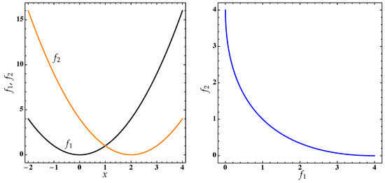
Figure 1.
Left: the objectives and from a multi-objective optimization problem (MOP; Equation (1)). Right: the corresponding Pareto set over the interval .
In many real-world applications, MOPs arise naturally. As one example, in almost all scheduling problems (e.g., References [36,37,38,39,40,41]), the total execution time (make-span) is of primary interest. However, the consideration of this objective is in many cases not enough since other quantities such as the tardiness or the energy consumption also play an important role and can consequently, according to the given problem, also add objectives to the resulting multi-objective problem.
For the numerical treatment of MOPs, there exist already many established approaches. For instance, there are mathematical programming techniques [29,42], point-wise iterative methods that are capable of detecting single local solutions of a given MOP. Via use of a clever sequence of these resulting scalar objective optimization problems, a suitable finite size approximation of the entire Pareto front can be computed in certain cases [43,44,45,46]. Multi-objective continuation methods take advantage of the fact that the Pareto set at least locally forms a manifold [47,48,49,50,51,52]. Starting with an initial (local) solution, further candidates are computed along the Pareto set of the given MOP. All of these methods typically yield high convergence rates but are, in turn, of local nature. A possible alternative is given by set oriented methods such as subdivision and cell mapping techniques [53,54] and evolutionary algorithms [55,56,57,58,59] that are of global nature and are capable of computing a finite size approximation of the Pareto front in one single run.
2.2. Finite Power Means
A comprehensive reference on the theory and properties of means is given in Reference [60], where proofs of the statements presented here for finite power means and for integral power means in the following subsection can be found (see also Reference [18] for integral means).
For a finite set and a nonzero real p, the p-average or the p power mean of A is given by
where denotes the cardinality of A. The simpler notation will also be employed. Moreover, in order to simplify the forthcoming expressions, we introduce the abbreviation
to denote the arithmetic mean of the elements of a finite set .
It is well known that limit cases of power means recover familiar quantities, for example,
is the standard geometric mean of the elements of A. The special case corresponds to the harmonic mean,
Moreover, the p-average of any finite set can also be defined for any p in the extended real line by taking appropriate limits.
Proposition 1.
Let A and B be finite subsets of and be arbitrary constants. Then, the following properties hold for finite power means:
- 1.
- .
- 2.
- For : .
- 3.
- For a matrix of nonnegative elements with and :
- 4.
- For :
- 5.
- For the harmonic mean: .
2.3. Integral Power Means in Measure Spaces
In order to present this part with sufficient generality, let us denote by a measure space. Let be the algebra of measurable subsets of and be the collection of those subsets with finite measure.
Now, we recall some fundamental properties of integral power means in this setting needed for the forthcoming sections. For and a measurable function defined on a subset , the p power mean or p-average of f over X is given by
For convenience, rhs of Equation (2) will be denoted simply as
where refers in this context to the measure of X and not to its cardinality as in the finite case. For brevity, when the measure employed is clear, will be abbreviated by to highlight the variable being integrated. The shorthand will also be employed.
For , the integral p mean corresponds to , where is the standard p norm of the Lebesgue space . The cases can also be included by taking the limits . In fact, since the essential supremum of the function f on X is , and when f is not identically zero its essential infimum is precisely ; by calculating the limits, we obtain that
and similarly,
Note that corresponds to the norm of the space . For , it is possible to define as the integral generalization of the notion of geometric mean, and it is given explicitly by
Proposition 2.
For subsets , nonnegative measurable functions , and any product-measurable function , the integral power mean satisfies that
- 1.
- For , : and .
- 2.
- For : .
- 3.
- For : .
- 4.
- For and : .
- 5.
- For with : .
3. The p-Averaged Hausdorff Distance
When trying to measure the distance between subsets of Euclidean space or even an arbitrary metric space, a natural choice is the well-known Hausdorff distance that is extensively employed in many different contexts. However, its use is of limited practical value to measure the distance to the Pareto set/front in typical MOPs, such as stochastic search methods implemented by an evolutionary algorithm. This is due to the fact that these algorithms may produce a set of outliers that can be heavily punished by . As a partial remedy, the use of an averaged Hausdorff distance was first proposed in Reference [16] to replace .
Let denote a distance function on a metric space for which the standard properties of the identity of indiscernibles, nonnegativity, symmetry, and subadditivity (more commonly known as the triangle inequality) are satisfied.
Definition 2.
Given a point and subsets , we have
- 1.
- A pointwise distance to sets: .
- 2.
- A pre-distance between sets: .
- 3.
- The Hausdorff distance between sets: .
For simplicity, throughout the text, the metric d can be assumed to be the standard Euclidean distance induced on some by the Euclidean 2 norm of , but the theory carries over to any general metric space .
Definition 3.
Let . For finite subsets , their (modified) p generational distance is
and their (modified) p inverted generational distance is
From them, the p averaged Hausdorff distance is obtained by taking the maximum
The indicators and in Definition 3 correspond to simple adjustments to the definitions of the generational distance [61] and the inverted generational distance [62].
The standard Hausdorff distance is recoverable from by taking the limit , but for any finite value of p, the distance is obtained from standard p power means of all the distances employed to calculate the supremum in part 2 of Definition 2, which is needed to define .
The advantage of using as an indicator is that it does not immediately disqualify a few outliers in a candidate set, contrary to what does and that, among the possible configurations of (finite) candidate solutions to a MOP, it assigns lesser distances to the Pareto front to those solutions appearing evenly spread along its whole domain (see, e.g., Reference [63]). The behavior of as a quality indicator is studied, e.g., in References [16,28], and it corresponds to the particular case of the results for general -indicators presented in Section 6.
Concerning its metric properties, has the drawback of not being a proper metric in the usual sense because for any non-unit set the distance . This problem will be fixed in the following section with a simple modification. Nevertheless, independently from that, for a positive number p, the distance does not satisfy the triangle inequality but only a weaker version of it. Indeed, as a consequence of Corollary 3, we have that
where and .
For further details concerning , its properties, and its relation to other indicators, the reader can consult, e.g., References [16,63].
4. The (p,q)-Averaged Hausdorff Distance
To better evaluate the optimality of a certain candidate set to approximate the Pareto set/front of a MOP, several generalizations of the averaged Hausdorff distance have been recently introduced.
4.1. (p,q)-Distances between Finite Sets
Definition 4.
For , the generational -distance between two finite subsets is given by
The distance can be extended for values of or , by taking the limits or , respectively. In such cases, properties of finite power means suggest the following definitions:
We can also calculate when or by changing the corresponding sum with a minimum or a maximum according to the case. In particular, we have the nice relation
Note that the definition of has two drawbacks, namely does not necessarily vanish if and in general , hence it does not define a proper metric. In order to get one, a slight modification is needed.
Definition 5.
Let . For finite subsets , their-averaged Hausdorff distance is
Notice that when , thus using Equation (3) and Definition 5, we easily obtain
In this way, for finite and disjoint sets, the indicator is a generalization of . Similarly to the relation
between the and the matrix norm of the distance matrix for and , we also have the following relation between the -generational distance and the matrix norm , where the definition of the latter is precisely that of but replacing all the normalized sums by standard ones ∑ (see, e.g., Reference [64]):
A useful property of the distance is that the parameters can be adjusted independently to achieve some desired spread of the archives by choosing an appropriate q and that they can be located with custom closeness to the Pareto front of a MOP by an adequate choice of p.
4.2. -Distances between Measurable Sets
With the aid of Proposition 2, the results of the previous section can be generalized to subsets of a metric space endowed with an appropriate measure . For concreteness, can be taken to be a subset of carrying the metric induced from the Euclidean metric of and endowed with an appropriate non-null measure . Notice that, in our intended applications, will not be the restriction of the standard Lebesgue measure of to for the simple reason that it can easily vanish as it happens on any hypersurface or lower dimensional subsets of . In this case, a lower dimensional measure is needed and alternatives like the Hausdorff measure on can be used, since it gives rise to the standard notion of d dimensional volume for d submanifolds of . When these submanifolds are parametrized by functions from subsets of , the same volume will be obtained by a change of variable formulae from the standard Lebesgue measure on those subsets of .
A very important observation in this context is that any set-theoretic relation obtained from measure-related calculations needs to be understood to hold almost everywhere (a.e.). Therefore, for , the statements or mean that the relations hold a.e., i.e., or , respectively. In other words, in this setting, we will always identify with its equivalence class . This means that those classes will be regarded as the elements of , removing the need to carry the abbreviation a.e. all the time. Henceforth, to simplify complicated formulae, will be shortened to .
Definition 6.
Let . For finite-measure subsets , their generational -distance is given by
The cases or are well defined only if X and Y are disjoint subsets.
Similarly to the finite case, can be extended to values of , but there are two drawbacks: only if X is a unit-set or singleton, and can differ from . To fix this undesirable behavior, we repeat the strategy used in the finite case as follows.
Definition 7.
Let . For finite-measure subsets , their -averaged Hausdorff distance is given by
Remark 1.
In general, the -distances are maps: . On the collection of finite subsets of , the standard counting measure can be taken as the underlying one needed for these measure-theoretic notions of and , and in this case, these distances become precisely the finite-case distances given in Definitions 4 and 5.
Remark 2.
For disjoint subsets X and Y, Definition 5 in the finite case and Definition 7 above in the measurable case reduce to the simpler form
which is the one we will actually use in most situations. The more general definition for non-disjoint subsets is given with the purpose that the distance so-defined changes continuously as one set approaches the other until their distance vanishes. In other words, the general definition allows the distance to become a continuous function with respect to the metric topology that it determines. Nevertheless, for practical purposes dealing with applications and for most of the results presented below, the simpler definition between disjoint subsets suffices.
5. Metric Properties
To explain some of the terminology used in this section, we recall to the reader that the standard triangle inequality for a distance function is usually weakened in two different but related ways by postulating the existence of a constant such that, for any points , one of the following conditions hold:
- The C relaxed triangle inequality: .
- The C inframetric inequality: .
Since the second condition implies the first one by using the very same constant and, reciprocally, the C relaxed triangle inequality implies the inframetric one, both conditions are equivalent for an appropriate choice of constants. A semimetric satisfying any one of these conditions will be simply called an inframetric.
For arbitrary measurable sets in , the following results summarize the metric properties of and . Using the counting measure, these properties also apply to finite sets. For more details, see Reference [17] in the finite case and Reference [18] in the generalized measure-theoretic context.
Theorem 1.
For , the generational -distance is subadditive in , i.e., for any , the triangle inequality holds true:
Proof.
The proof follows easily by simple steps using the properties in Proposition 2. We start from the standard triangle inequality for :
taking at both sides the q-average over Z and using 1–3 of Proposition 2 to arrive at
Now, there are two independent cases for the parameters . We explain here only the case , but the case follows by similar arguments; see Thm. 2 in Reference [18]. Calculating the p-average over X at both sides of Equation (4) and using 1, 3, and 5 of Proposition 2, we get
Since the lhs of Equation (5) is , after a further p-average over Y at both sides of Equation (5) and parts 1, 3, and 5 of Proposition 2, we obtain
But from 2, 4, and 5 of Proposition 2, the first term at the rhs above satisfies
Corollary 1.
If , the -averaged Hausdorff distance is a semimetric on the space of finite-measure subsets of . Furthermore, if the distance behaves as a proper metric when it is restricted to disjoint subsets of .
Proof.
From Definition 7, we obtain the relations and for any and all . Moreover, from Definition 6, it follows that if and only if or (hence, ). Therefore, for ,
i.e., is a semimetric on the collection of finite-measure subsets . Finally, for disjoint X and Y, it is clear that ; thus, by Theorem 1, the triangle inequality holds for both arguments inside the maximum that defines when . This implies that the triangle inequality is also valid for . □
Theorem 2.
Let be subsets admitting positive constants such that for any and . Then, for all , and at least one of them negative a relaxed triangle inequality holds for , namely
Proof.
Step 1: Let , and suppose that . We will prove that
For all and , we have . Thus,
Since , this means that . Taking the p-average at both sides and from 1 and 4 of Proposition 2, we find , which is exactly Equation (6).
Step 2: Now, for and , we will prove that
By assumption, we have for any and all . Similarly as before and using 1 and 4 of Proposition 2, we conclude from the rhs part that . However, since , after taking a p-average of the quotient of means, it follows from
that , which is now (7).
Step 3: The previous steps can be summarized in the expression
Using again 4 of Proposition 2 and Definition 6, we get . From this, the subadditivity for (Theorem 1), and Equation (8), we conclude
□
Remark 3.
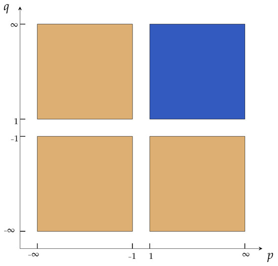
For parameters that lie in the orange or blue sectors in Figure 2, the distance fulfills a C relaxed triangle inequality for a constant only if the condition holds for all and . On bounded and topologically separated sets (i.e., not having common limit points), this condition always holds, and on them, becomes an inframetric as explained below.

Figure 2.
According to Corollary 1, when acting on disjoint subsets, behaves as a proper metric if lies in the blue sector, and according to Corollary 2, it behaves like an inframetric if lies in the orange sectors.
Corollary 2.
Under the same hypotheses of Theorem 2, the -averaged Hausdorff distance satisfies
Proof.
It is immediate using Theorem 2 and Definition 7. □
When the involved sets are finite, a generally sharper inframetric relation holds. For emphasis, we employ in this context the notation for those subsets of .
Theorem 3.
If and , the -distance satisfies the relaxed triangle inequality
for all finite subsets , where and .
Proof.
For arbitrary , let us assume that , so that . We can write
which, when combined with property 5 of Proposition 1, yields
A similar relation is true for any if . In conclusion, , where
If does not need to be sharp, can always be chosen to take the larger value .
Now, for , the final result follows from the triangle inequality for :
Corollary 3.
If and , the -distance satisfies the relaxed triangle inequality:
for all finite subsets , with , and .
Proof.
The corollary follows immediately from Theorem 3 and Definition 5. □
To conclude this section, we return to the general setting of arbitrary measurable sets to explain the behavior of when changing the value of its parameters p and q.
Theorem 4.
Let and suppose that satisfy and . Then,
Proof.
It follows easily from part 5 of Proposition 2 and Definition 7. □
6. The (p,q)-Distances as Quality Indicators
Let Q be a decision space Q and be a multi-objective function on it, of which the associated MOP consists in the simultaneous minimization of its k component functions . A candidate solution to this problem is Pareto-optimal if all elements of its image in are nondominated in the sense of Pareto [31]; see Definition 1. For the forthcoming discussion, let us introduce the following abbreviated and useful notation. For and any , we define the following
From these definitions, it follows that, for arbitrary and , there are partitions:
where ⊔ stands for the disjoint union of subsets. A similar notation with the subindices ≺, ≻, and ⪰ can also be used in an analogous way. Let us recall that an archive is, by definition, a subset of mutually non-dominated points; therefore, for any , the condition implies . This basic property implies that is a bijection when restricted to any archive and, therefore, the points in can be univocally labeled by the elements of X. Moreover, for a finite archive , both sets have the same number of elements .
Now, we introduce a couple of strengthened notions of dominance between sets (archives) that are required for the validity of most of the results in this section.
Definition 8.
An archive X is well-dominated by an archive Y if
- 1.
- X is dominated by Y, written , i.e., , s.t. , and
- 2.
- Y consists only of dominating points of X, i.e., , s.t. .
Moreover, X is said to be strictly well dominated by Y if
- 3.
- , such that .
For an archive , the , , and quality (or performance) indicators assigned to it will be defined as the distance of its image to the Pareto front , i.e.,
In this section, we study the behavior of , , and as performance indicators. An example of a weakly Pareto-compliant performance indicator is the Degree of Approximation (DOA; see Reference [10]).
6.1. Pareto Compliance of -Indicators in the Finite Case
In order to obtain general conclusions on the features of the averaged Hausdorff distance as a quality indicator, we consider first the behavior of . For additional details on the material presented in this section and other related results in the context of the p-averaged Hausdorff Distance , the reader is referred to Reference [28].
For the following statements, we will abbreviate . Clearly, with this notation, , where in the averaged sum , we are labeling the points in by the elements of the archive A, taking advantage of the fact that , as it also will be done with all the averages in this section.
Theorem 5.
Let be finite archives with A strictly well dominated by B. For all and ,
- 1.
- implies that ;
- 2.
- implies that (or equivalently an strict equality);
then, .
Proof.
By condition 1, for all and , the inequality holds true. After averaging over all at both sides, we have
and averaging once again over all produces
From property 2 and noticing that each appears times in the initial sum, the lhs becomes
Returning to Equation (9), we conclude that . Lastly, part 3 of Definition 8 for strictly well-dominated sets guarantees that this is an strict inequality, proving the assertion. □
Remark 4.
Since we are dealing with finite archives, condition 2 of Theorem 5 regarding the relative size of some of their parts is equivalent to the condition regarding the relative size of their images. This is not necessarily the case in the context of measurable subsets, but see Remark 5.
Figure 3 shows examples where Theorem 5 holds with . In this case, the q-averaged distance becomes the standard distance between a point and a set.
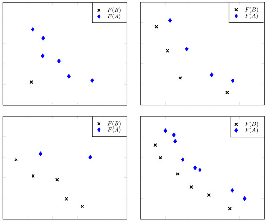
Figure 3.
Different scenarios where the value of archive B is better (smaller) than the value of archive A independently of the Pareto set and where the additional assumptions made in Theorem 5 are easily verifiable.
For the inverted generational distance in the finite case, we provide here two useful results without explicit proofs. The necessary steps are similar to the arguments used to prove the analogous statements for in Prop. 3.8 of Reference [28] and Thm. 3.9 in Reference [28]. Those statements correspond here to the limit , and the main difference in the proofs is that the Euclidean distante needs to be changed everywhere by the q-average , as it was done above for the proof of Theorem 5 that generalizes the proof of Thm. 3.4 in Reference [28]. The reader can also find there additional remarks on similar hypotheses to the ones needed for Theorem 6 below.
Proposition 3.
Let be finite and strictly well-dominated archives with such that for all , , and :
then, .
Figure 4 illustrates two situations where the hypotheses of Proposition 3 are satisfied. Now, to state a more general result concerning the Pareto compliance of the indicator, we will further abbreviate the minimal p-average of distances by
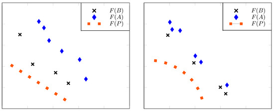
Figure 4.
Two situations where is better (smaller) than for sufficiently negative q: Here, the hypotheses of Proposition 3 hold true.
Theorem 6.
Let be finite and strictly well-dominated archives such that . If at least one of the following conditions is satisfied,
- 1.
- , : ;
- 2.
- such that : ;
- 3.
- : ;
then .
Finally, a general statement on the Pareto compliance of the finite case of the -averaged Hausdorff distance follows as a consequence of Theorems 5 and 6.
Theorem 7.
Let be finite and well-dominated archives such that . If for all , :
and at least one of the following conditions is satisfied:
- 1.
- , , : ;
- 2.
- such that : ;
- 3.
- : ;
then, .
Figure 5 illustrates four situations where Theorems 6 and 7 apply with very large q. In the first row, the left diagram is a modification of the second case in Figure 4 where condition 1 holds. In the right diagram, the diamond lying at the lower left corner of represents the image of a point satisfying condition 2. Finally, both diagrams in the second row exhibit cases where the points of are equidistant to corresponding points in , making condition 3 valid, with being this distance.
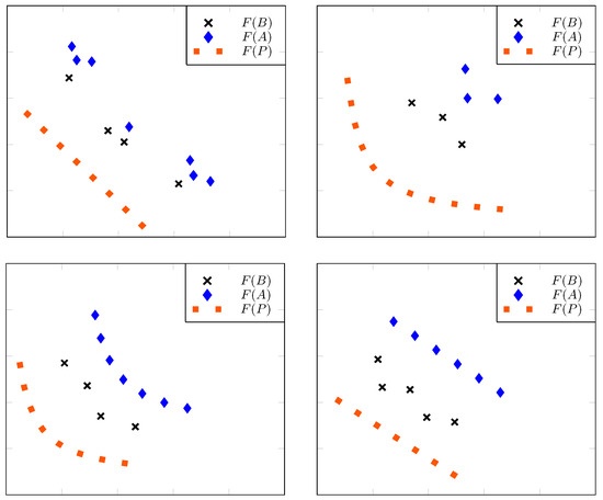
Figure 5.
Four examples where is smaller (better) than for sufficiently negative q: In each case, at least one of the requirements of Theorem 6 is satisfied.
6.2. Pareto Compliance of -Indicators in the General Case
We consider now the behavior of the generalized distance with respect to the Pareto-compliance, concentrating on the most important aspects that describe its characteristics and using similar hypotheses to the ones needed in the previous section for in the finite case.
Here, we will continue to assume that the decision space Q with objective function defining the MOP under consideration has a Pareto set with corresponding Pareto front . Also, we assume that the objective space carries a metric d that, for simplicity, can be taken to be the one inherited from the Euclidean distance in . In addition, to define the -indicators on MOPs that require general non-finite sets, we need a measure space , that here will be taken to be endowed with a non-null measure according to the comments at the beginning of Section 4.2. In this context X, will denote arbitrary subsets such that are measurable with non-null and finite measures.
Remark 5.
Recall that, here, denotes the measure of . In this context, Q will not be asked to carry a measure and the notation will have no a priori meaning for . Nevertheless, it is possible to induce a measure on those subsets of Q where F is bijective by taking the pullback of μ to them, making the identity trivially true. This can be done for all archives but not for subsets where F is not bijective. When it is Q that carries a measure, a push-forward measure can be always defined on its image , making this identity true for all sets. This was implicitly assumed in the presentation provided in Reference [18] (Section 3.4). For clarity, we avoid here this identification and state everything from the assumption that the measure μ is defined only on .
Before stating the complete result, let us recall that a partition of a set X is a collection of disjoint and non-empty subsets of X whose union is the whole of X and a partition of an archive induces a partition of by the bijectivity of F restricted to X. For convenience, we abbreviate the measure-theoretic q-averaged distance from a point to a set by .
Theorem 8.
For , let denote archives of which the images and are of non-null finite measures in . Moreover, assume that
- 1.
- there exist finite partitions and such that :
- (a)
- and are subsets of non-null finite measure in ;
- (b)
- , : ;
- 2.
- , : ;
then, .
Proof.
By of Theorem 8, the sets X and Y can be subdivided into the same number m of subsets, and by , if and for any , then . Therefore, we can take successive integral p-averages over and, afterwards, over at both sides of this inequality to find that, for each i, we have
For those violating the inequality , we subdivide into a sufficiently large partition of subsets , with images by F of non-null finite measure, so as to guarantee that, for all , we get
Notice that this is indeed possible because each is of non-null finite measure. Since , , we have , an inequality similar to Equation (10) also holds for them, i.e.,
for all , . However, , where and . Therefore, with the notation of Equation (11), a simple calculation shows that , implying that and are normalized weights useful for weighted averages. Since and , simple properties of discrete weighted power mean imply the inequality . Thus, we can finally write
□
Remark 6.
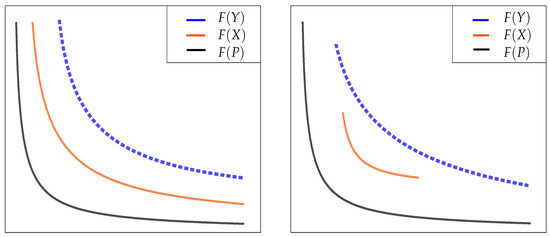
From condition 1 of Theorem 8, it follows the simpler (and somewhat weaker) dominance conditions:
- ()
- (i.e., , such that ), and
- ()
- , such that .
For simple situations where () and () are valid, the partitions needed for part 1 of Theorem 8 are not difficult to find; however, this is not always possible as the right side of Figure 6 indicates. Indeed, Figure 6 presents some examples where () and () hold true, but can be both true (left side) and false (right side). Furthermore, it is possible to show that X and Y comply (left side) and do not comply (right side) with condition 1 of Theorem 8, respectively.

Figure 6.
(Left) A situation where the Pareto front and the images and of continuous archives satisfy and condition 1(a) of Theorem 8 holds true. (Right) A modification of the previous situation where conditions and of Remark 6 are satisfied but . Here, there are no possible partitions of the archives satisfying part 1(a) of Theorem 8.
Remark 7.
An important advantage of using over is that condition 2 of Theorem 8 provides the possibility of choosing an appropriate for which the condition holds when , ensuring in this way the compliance to Pareto optimality for . This freedom is lacking for because, in the limit , the distance becomes the standard distance , which does not allow for any choice.
7. Examples and Numerical Experiments
In this section, we present some numerical experiments involving finite sets first, and afterwards, we study the case of continuous sets.
7.1. Working with over Finite Sets
Let us take a hypothetical Pareto front P given by the line segment from to in , i.e., the set of all points
This is the same example considered in Reference [16] p. 506 and enables us to make a comparison with values of . In order to use the finite version of , we discretize P by taking 11 uniformly distributed points; we call this set . We assume two archives: is obtained from by changing for , including an outlier, and by adding to the remaining ordinates. is obtained from by adding 5 to each ordinate. See Figure 7.
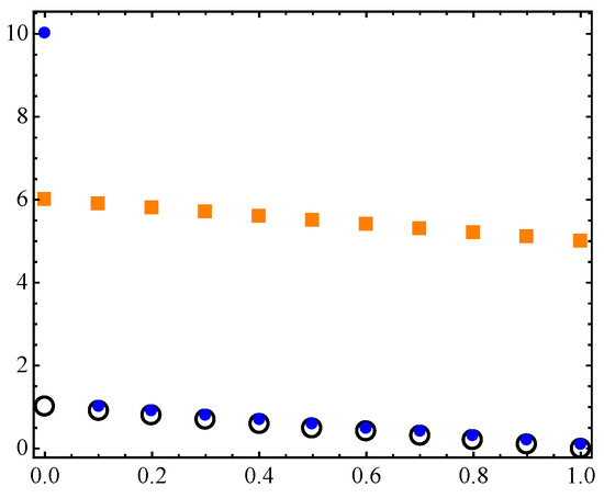
Figure 7.
A hypothetical Pareto front discretization (black circles) and two different archives: (blue dots) and (orange squares).
As explained in Section 3, we know that
coincides with the standard Hausdorff distance . In this case, we obtained
and according to Theorem 4 and Reference [16] p. 512, these values must increase as p increases.
Table 1 and Table 2 show that we can find values of p and q such that the -averaged distance does not punish heavily the outliers, for example, or and . We remark that the values of do not present a significative change under variations of for a fixed p. Thus, it is possible to work with , in which case is a metric according to Corollary 1, and to still obtain values close to the ones given by the inframetric , with the same .

Table 1.
for several values of p and q.

Table 2.
for several values of p and q.
For large values of p, the behavior of presents the same disadvantages of or of the standard Hausdorff distance. For example, in Table 1 and Table 2, it can be observed that all distances for are useless because they imply that the distance from the discrete Pareto front to the archive is larger than its distance to the archive . Figure 7 suggests that this is an undesirable outcome.
Table 3 shows that is close to a metric when and . The percentage of triangle inequality violations decreases as p increases or q decreases.

Table 3.
Triangle inequality violations, in percentage, for several values of p and q: Here, we randomly chose 80 sets, each one containing 2 points in , and verified the triangle inequality for all possible set permutations (that is, 492,960).
7.2. Optimal Archives for Discretized Spherical Pareto Fronts
We now consider two standard Pareto fronts: The spheric convex and spheric concave quarter-circles, see Figure 8 and Figure 9.
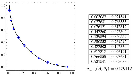
Figure 8.
Optimal archive A for the connected Pareto front given by Equation (12) with 10 elements (blue circles) and at the right is the respective archive coordinates and the distance.
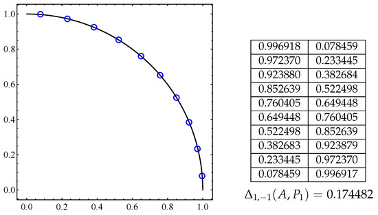
Figure 9.
Optimal archive A for the connected Pareto front given by Equation (12) with 10 elements (blue circles) and at the right is the respective archive coordinates and the distance.
To numerically find the optimal archive of size M, we discretized the Pareto front with 1000 equidistant points (which is an acceptable discretization according to Reference [63] p. 603) and randomly chose an initial M sized archive. Then, we used a random-walk (or step climber) evolutionary algorithm, moving one point at a time. Finally, we refined the optimal archive with the “evenly spaced” construction suggested by Reference [63] p. 607.
When finding optimal archives, our numerical experiments suggest a clear geometrical influence of the parameters p and q. For values of p in , the optimal archive sets are basically the same. When increases, the optimal archive tends to lose dispersion, converging to one point. When , the optimal archive collapses to one point, and when , the corresponding optimal archives are basically the same (see Figure 10). When increases, the optimal archive moves away from the Pareto set (see Figure 11).
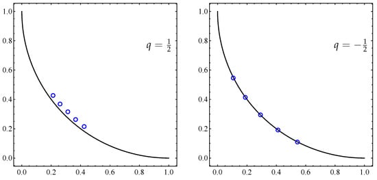
Figure 10.
Optimal five-point set archives A for the connected Pareto front given by Equation (12) with and .
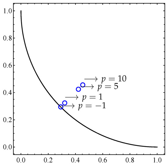
Figure 11.
Optimal one-point archives A for the connected Pareto front given by Equation (12) with and different values of p: In all cases, the archives are located in the line .
7.3. Optimal Archives for Disconnected and Discretized Pareto Sets
In this section, we present the optimal archives for a disconnected step Pareto front:
where s is the number of steps, is a small constant responsible for the step’s twist, and stands for the integer part function.
Figure 12 shows numerical optimal archives of sizes 20. The archive coordinates reveal that
i.e., the optimal archive points do not lie over the Pareto front but they are so close to it that this is hardly noticeable. It is also evident that the archives are evenly distributed along the Pareto front.
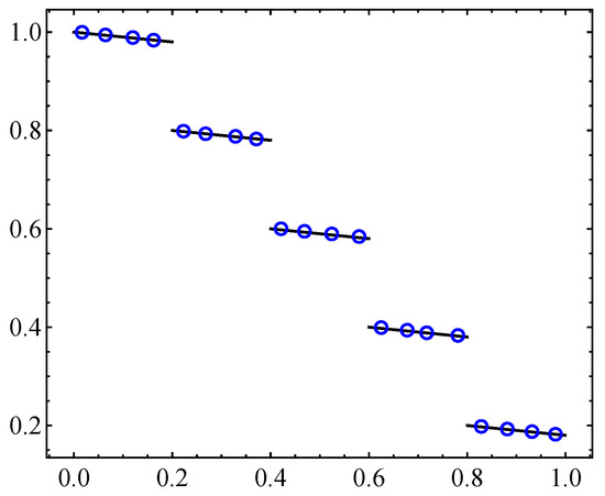
Figure 12.
Numerical optimal archive A for the disconnect step Pareto front given by Equation (13) with 20 elements: here, we obtain .
7.4. General Example for Continuous Sets
In this first example, we are going to construct simple and illustrative continuous sets A and B. Let A be the straight segment in from to , that is
For a small positive and a variable , let be the set given by the following union of straight segments
where , , , , , and . We can regard the set as a continuous approximation of A, where the central segment can be seen as the outlier.
In the following Figure 13, we can see the sets A and for and . According to Table 4, as decreases, the distance between the approximation and the set A also decreases.
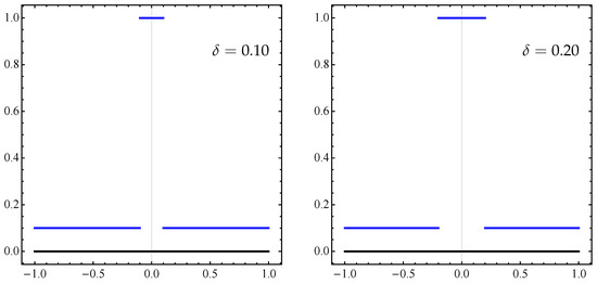
Figure 13.
The black horizontal segment is the set A from Equation (14), and the blue piecewise map is the respective approximation given by the set from Equation (15) for two values of and .

Table 4.
results between the sets A and in Equations (14) and (15) for and some parameter values of p, q, and .
We remark that the classical Hausdorff distance between A and produces the value 1 for any . Thus, by working with the -distance instead of , we can detect “better” approximations.
7.5. Approximating Pareto Set and Front of a MOP
Finally, we address the problem to approximate the Pareto sets and fronts of given MOPs. As an example, we will consider the bi-objective Lamé super-sphere problem [32] which is defined as follows:
where is defined as
where and . For , the Pareto sets and fronts of this problem are shown in Figure 14 and Figure 15 for and , respectively.
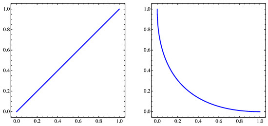
Figure 14.
(Left) Pareto set. (Right) Pareto front of MOP (Equation (16)) for and .
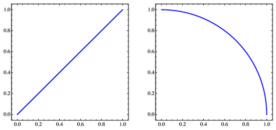
Figure 15.
The same as in Figure 14 but for .
In a first step, we discuss the principle difference of discrete and continuous archives when approximating the Pareto set/front on a hypothetical example. For this, we assume that we are given the 5-element archive ; those elements are given by
Hence, we can see A as a 5-element approximation of the Pareto set and its image as a 5-element approximation of the Pareto front. Now, instead of A, we may use a polygonal curve that is defined by A:
In the following, we will call A a discrete archive while we call the polygon approximation B the continuous archive. Figure 16 and Figure 17 show the approximations A and B as well as their images and . Apparently, the approximation qualities are much better for the linear interpolates. This impression gets confirmed by the values of for this problem that are shown in Table 5. We can observe the following two behaviors: (i) the distances are much better for the continuous archives and the differences are even larger in objective space, and (ii) the distances decrease with decreasing q (which is in accordance to the result of Theorem 4).
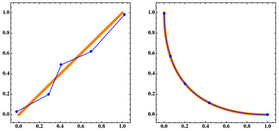
Figure 16.
(Left) The blue dots A and the blue polygonal line B are the discrete and continuous approximations, respectively, for the Pareto set which corresponds to the orange thick segment, of MOP (Equation (16)) for . (Right) respective sets and of the Pareto front for .
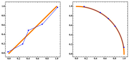
Figure 17.
The same as in Figure 16 but for .

Table 5.
results for the approximations of the Pareto set and front for MOP (Equation (16)).
In a next step, we consider discrete archives that have been generated from multi-objective evolutionary algorithms together with their resulting continuous archives. For multi-objective evolutionary algorithms, we have chosen the widely used methods NSGA-II [65] and MOEA/D [66]. We stress, however, that any other MOEA could be chosen and that the conclusions we draw out by our results apply in principle to any other such algorithm. Table 6 shows the parameter setting we have used for our studies.

Table 6.
Parameter setting for NSGA-II and MOEA/D: Here, n denotes the dimension of the decision variable space.
Figure 18 and Figure 19 and Table 7 show the results of NSGA-II where we have used 500 generations and a population size of 12. Figure 20 and Figure 21 and Table 8 show the respective results for MOEA/D where we have also used 500 generations and population size 12. We can see that, for both algorithms, the values are significantly better for the continuous archives. We can also make another observation: the values oscillate for the results of the dominance-based algorithm NSGA-II which is indeed typical. For the continuous archives, these oscillations are less notorious, which indicates that the use of continuous archives may have a smoothing effect on the approximations, which is highly desired.
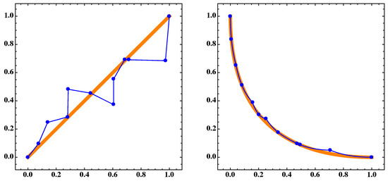
Figure 18.
(Left) the blue dots A and the blue polygonal line are the discrete and continuous approximations, respectively, for the Pareto set and the orange thick segment is for the 410th generation of the NSGA-II algorithm of MOP (Equation (16)) for . (Right) corresponding sets and of the Pareto front for .
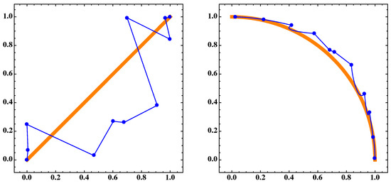
Figure 19.
The same as in Figure 18 but for .

Table 7.
For MOP (Equation (16)), the Table shows the results for the finite and continuous Pareto front approximations. We used the NSGA-II generated archives for and .
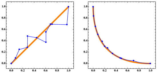
Figure 20.
(Left) the blue dots A and the blue polygonal line are the discrete and continuous approximations, respectively, for the Pareto set and the orange thick segment is for the 410th generation of the MOEA/D algorithm of MOP (Equation (17)) for . (Right) corresponding sets and of the Pareto front for .
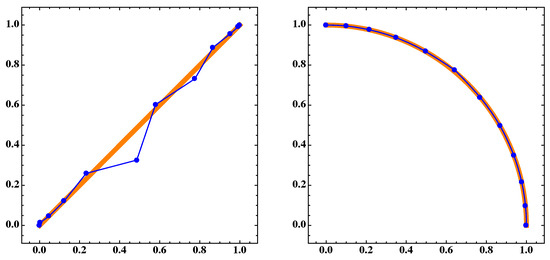
Figure 21.
The same as in Figure 20 but for .

Table 8.
For MOP (Equation (16)), the Table shows the results for the finite and continuous Pareto front approximations. We used the MOEA/D generated archives for and .
We want to investigate the last statement further on. To this end, we consider the following convex bi-objective problem: the objectives are given by , where
Figure 22 shows the Pareto set and front of MOP (Equation (17)). The Pareto set is given by the straight segment joining and .
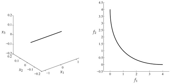
Figure 22.
(Left) Pareto set. (Right) Pareto front of MOP (Equation (17)).
The values of obtained by NSGA-II for the discrete archives (using population size 20) as well as for the respective continuous archives can be seen in Figure 23 and Table 9. Also for this example, the values for the continuous archives are much better and the oscillations are significantly reduced compared to the discrete archives.
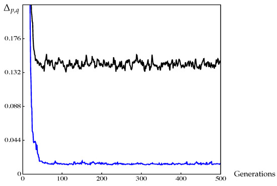
Figure 23.
The black curve is the value for the discrete approximation, and the blue one is the respective curve for the continuous approximation of NSGA-II for MOP (Equation (17)).

Table 9.
results between the Pareto Front and its respective discrete and continuous approximations of NSGA-II for MOP (Equation (17)): The data shown is the averaged over the 20 independent runs above.
Figure 24, Figure 25 and Figure 26 show the results of both kinds of archives after 300, 400, and 500 generations which confirm this observation. The results show that NSGA-II is indeed capable of computing points near the Pareto front while the distribution of the points vary. This is a known fact since there exists no “limit archive” for this algorithm (as it is, e.g., not based on the averaged Hausdorff distance or any other performance indicator). When considering the respective results of the continuous archives, however, NSGA-II computes (at least visually) nearly perfect approximations of the Pareto front. The values reflect this.
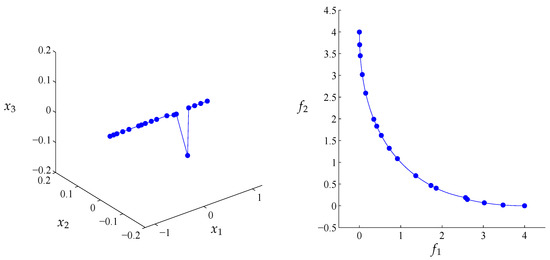
Figure 24.
(Left) The blue dots and the blue polygon line are the discrete and continuous approximation, respectively, for the Pareto set of MOP (Equation (17)) in the 300th generation. (Right) respective sets and of the Pareto front.
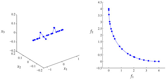
Figure 25.
The same as in Figure 24 but for the 400th generation.
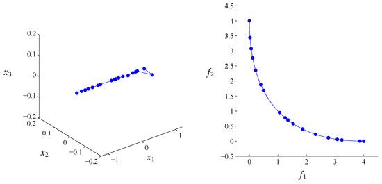
Figure 26.
The same as in Figure 24 but for the 500th generation.
8. Conclusions and Perspectives
In this paper, we have presented a comprehensive overview of the averaged Hausdorff distances that have recently appeared in connection with the study of MOPs.
Among the averaged Hausdorff distances studied here, the generalized as defined for arbitrary measurable sets was shown to provide a general and robust definition for applications that carries good metric properties, is adequate for use with continuous approximations of the Pareto set of a MOP, and even reduces to the previously introduced definition for discrete approximations.
Concerning the appearance of the additional parameter q in the definition of which could give the impression of an overly complicated expression, it is important to highlight, as it was observed in Remark 7, that it can provide the possibility to choose a suitable value of q in order to make as Pareto compliant as possible for the MOP under consideration. This is an argument in favor of the flexibility provided by the generalized version , which is not available for the distance, and this particular aspect worths further investigation.
Nevertheless, since the freedom provided by the two parameters p and q may appear as excessive and perhaps undesirable in many applications, there remains to find a practical recipe to determine and fix these parameters according to the characteristics of the problem under consideration. Certainly, the desired spreads of the optimal archives, the distance of an approximation to the Pareto front, and the convexity of these fronts need to be taken into account in order to determine an appropriate set of preferred values for these parameters depending on the situation.
To achieve these aims, more theoretical as well as numerical studies of optimal solutions associated with Pareto fronts with different convexities must be carried out and experiments evaluating how the Pareto compliance can be enhanced in each situation by the choice of parameters need to be performed.
Finally, we stress that the results we have shown in Section 7 show the advantage of a new performance indicator that is able to compute the performance of a continuous approximation of the solution set. Continuous approximations, e.g., of the Pareto set/front of multi-objective optimization problems have not been considered so far, though both Pareto set and front typically form continuous sets in case the objectives are continuous. The examples have indicated that the consideration of continuous archives (via use of interpolation on the populations generated by the evolutionary algorithms) could allow a reduction in population sizes and, hence, a significant reduction of the computational effort of the evolutionary algorithms. This is because the time complexity for all existing multi-objective evolutionary algorithms is quadratic in the population size and in each generation of the algorithm. To verify this statement, more computations are needed, which is left for future work.
Author Contributions
J.M.B. and A.V. obtained the theoretical results concerning the -averaged Hausdorff distance, and O.S. conceived and designed the experiments; J.M.B. and A.V. performed the experiments and provided the related figures and tables; O.S. analyzed the data and contributed with the text. J.M.B. and A.V. wrote the paper.
Funding
The first two authors were partially supported by Vicerrectoría de Investigación, Pontificia Universidad Javeriana, Bogotá D.C., Colombia. The third author was supported by Conacyt Basic Science project No. 285599 and SEP Cinvestav project no. 231.
Conflicts of Interest
The authors declare no conflict of interest.
References
- Heinonen, J. Lectures on Analysis on Metric Spaces; Springer: New York, NY, USA, 2001. [Google Scholar]
- de Carvalho, F.; de Souza, R.; Chavent, M.; Lechevallier, Y. Adaptive Hausdorff distances and dynamic clustering of symbolic interval data. Pattern Recogn. Lett. 2006, 27, 167–179. [Google Scholar] [CrossRef]
- Huttenlocher, D.P.; Klanderman, G.A.; Rucklidge, W.A. Comparing images using the Hausdorff distance. IEEE Trans. Pattern Anal. Mach. Intell. 1993, 15, 850–863. [Google Scholar] [CrossRef]
- Yi, X.; Camps, O.I. Line-based recognition using a multidimensional Hausdorff distance. IEEE Trans. Pattern Anal. Mach. Intell. 1999, 21, 901–916. [Google Scholar]
- Falconer, K. Fractal Geometry: Mathematical Foundations and Applications, 2nd ed.; Mathematical foundations and applications; John Wiley & Sons, Inc.: Hoboken, NJ, USA, 2003. [Google Scholar]
- Aulbach, B.; Rasmussen, M.; Siegmund, S. Approximation of attractors of nonautonomous dynamical systems. Discrete Contin. Dyn. Syst. Ser. B 2005, 5, 215–238. [Google Scholar]
- Dellnitz, M.; Hohmann, A. A subdivision algorithm for the computation of unstable manifolds and global attractors. Numerische Mathematik 1997, 75, 293–317. [Google Scholar] [CrossRef]
- Emmerich, M.; Deutz, A.H. Test problems based on Lamé superspheres. In Proceedings of the 4th International Conference on Evolutionary Multi-criterion Optimization EMO’07, Matsushima, Japan, 5–8 March 2007; Springer: Berlin/Heidelberg, Germany, 2007; pp. 922–936. [Google Scholar]
- Dellnitz, M.; Schütze, O.; Hestermeyer, T. Covering Pareto sets by multilevel subdivision techniques. J. Optim. Theory Appl. 2005, 124, 113–155. [Google Scholar] [CrossRef]
- Dilettoso, E.; Rizzo, S.A.; Salerno, N. A weakly Pareto compliant quality indicator. Math. Comput. Appl. 2017, 22, 25. [Google Scholar] [CrossRef]
- Padberg, K. Numerical Analysis of Transport in Dynamical Systems. Ph.D. Thesis, University of Paderborn, Paderborn, Germany, 2005. [Google Scholar]
- Peitz, S.; Dellnitz, M. A survey of recent trends in multiobjective optimal control—Surrogate models, feedback control and objective reduction. Math. Comput. Appl. 2018, 23, 30. [Google Scholar] [CrossRef]
- Schütze, O. Set Oriented Methods for Global Optimization. Ph.D. Thesis, University of Paderborn, Paderborn, Germany, 2004. [Google Scholar]
- Schütze, O.; Coello Coello, C.A.; Mostaghim, S.; Talbi, E.G.; Dellnitz, M. Hybridizing evolutionary strategies with continuation methods for solving multi-objective problems. Eng. Optim. 2008, 40, 383–402. [Google Scholar] [CrossRef]
- Schütze, O.; Laumanns, M.; Coello Coello, C.A.; Dellnitz, M.; Talbi, E.G. Convergence of stochastic search algorithms to finite size Pareto set approximations. J. Glob. Optim. 2008, 41, 559–577. [Google Scholar] [CrossRef]
- Schütze, O.; Esquivel, X.; Lara, A.; Coello Coello, C.A. Using the averaged Hausdorff distance as a performance measure in evolutionary multiobjective optimization. IEEE Trans. Evol. Comput. 2012, 16, 504–522. [Google Scholar] [CrossRef]
- Vargas, A.; Bogoya, J.M. A generalization of the averaged Hausdorff distance. Computación y Sistemas 2018, 22, 331–345. [Google Scholar] [CrossRef]
- Bogoya, J.M.; Vargas, A.; Cuate, O.; Schütze, O. A (p,q)-averaged Hausdorff distance for arbitrary measurable sets. Math. Comput. Appl. 2018, 23, 51. [Google Scholar] [CrossRef]
- Cai, X.; Li, Y.; Fan, Z.; Zhang, Q. An external archive guided multiobjective evolutionary algorithm based on decomposition for combinatorial optimization. IEEE Trans. Evolut. Comput. 2015, 19, 508–523. [Google Scholar]
- Shang, R.; Wang, Y.; Wang, J.; Jiao, L.; Wang, S.; Qi, L. A multi-population cooperative coevolutionary algorithm for multi-objective capacitated arc routing problem. Inf. Sci. 2014, 277, 609–642. [Google Scholar] [CrossRef]
- Zhang, J.; Tang, Q.; Li, P.; Deng, D.; Chen, Y. A modified MOEA/D approach to the solution of multi-objective optimal power flow problem. Appl. Soft Comput. 2016, 47, 494–514. [Google Scholar] [CrossRef]
- Dhiman, G.; Kumar, V. Multi-objective spotted hyena optimizer: A Multi-objective optimization algorithm for engineering problems. Knowl. Based Syst. 2018, 150, 175–197. [Google Scholar] [CrossRef]
- López-Rubio, F.J.; López-Rubio, E. Features for stochastic approximation based foreground detection. Comput. Vision Image Underst. 2015, 133, 30–50. [Google Scholar] [CrossRef]
- Kerkhove, L.P.; Vanhoucke, M. Incentive contract design for projects: The owner’s perspective. Omega 2016, 62, 93–114. [Google Scholar] [CrossRef]
- Hansen, M.P.; Jaszkiewicz, A. Evaluating the Quality of Approximations to the Non-Dominated Set; IMM, Department of Mathematical Modelling, Technical University of Denmark: Kongens Lyngby, Denmark, 1998. [Google Scholar]
- Zitzler, E.; Thiele, L. Multiobjective evolutionary algorithms: A comparative case study and the strength Pareto approach. IEEE Trans. Evol. Comput. 1999, 3, 257–271. [Google Scholar] [CrossRef]
- Siwel, J.; Yew-Soon, O.; Jie, Z.; Liang, F. Consistencies and contradictions of performance metrics in multiobjective optimization. IEEE Trans. Evol. Comput. 2014, 44, 2329–2404. [Google Scholar]
- Vargas, A. On the Pareto compliance of the averaged Hausdorff distance as a performance indicator. Universitas Scientiarum 2018, 23, 333–354. [Google Scholar] [CrossRef]
- Miettinen, K. Nonlinear Multiobjective Optimization; Kluwer Academic Publishers: Tranbjerg, Denmark, 1999. [Google Scholar]
- Ehrgott, M.; Wiecek, M.M. Multiobjective programming. In Multiple Criteria Decision Analysis: State of the Art Surveys; Springer: New York, NY, USA, 2005; pp. 667–722. [Google Scholar]
- Pareto, V. Manual of Political Economy; The Macmillan Press: London, UK, 1971. [Google Scholar]
- Hillermeier, C. Nonlinear Multiobjective Optimization: A Generalized Homotopy Approach; Springer Science & Business Media: Berlin, Germany, 2001; Volume 135. [Google Scholar]
- Köppen, M.; Yoshida, K. Many-objective particle swarm optimization by gradual leader selection. In Proceedings of the 8th international conference on adaptive and natural computing algorithms (ICANNGA 2007), Warsaw, Poland, 11–14 April 2007; Springer: Berlin/Heidelberg, Germany, 2007; pp. 323–331. [Google Scholar]
- Schütze, O.; Lara, A.; Coello Coello, C.A. On the influence of the number of objectives on the hardness of a multiobjective optimization problem. IEEE Trans. Evolut. Comput. 2011, 15, 444–455. [Google Scholar] [CrossRef]
- Schaffer, J.D. Multiple Objective Optimization with Vector Evaluated Genetic Algorithms. Ph.D. Thesis, Vanderbilt University, Nashville, TN, USA, 1984. [Google Scholar]
- Amini, A.; Tavakkoli-Moghaddam, R. A bi-objective truck scheduling problem in a cross-docking center with probability of breakdown for trucks. Comput. Ind. Eng. 2016, 96, 180–191. [Google Scholar] [CrossRef]
- Li, M.W.; Hong, W.C.; Geng, J.; Wang, J. Berth and quay crane coordinated scheduling using multi-objective chaos cloud particle swarm optimization algorithm. Neural Comput. Appl. 2017, 28, 3163–3182. [Google Scholar] [CrossRef]
- Dulebenets, M.A. A comprehensive multi-objective optimization model for the vessel scheduling problem in liner shipping. Int. J. Prod. Econ. 2018, 196, 293–318. [Google Scholar] [CrossRef]
- Goodarzi, A.H.; Nahavandi, N.; Hessameddin, S. A multi-objective imperialist competitive algorithm for vehicle routing problem in cross-docking networks with time windows. J. Ind. Syst. Eng. 2018, 11, 1–23. [Google Scholar]
- Venturini, G.; Iris, C.; Kontovas, C.A.; Larsen, A. The multi-port berth allocation problem with speed optimization and emission considerations. Transp. Res.Part D Transp. Environ. 2017, 54, 142–159. [Google Scholar] [CrossRef]
- Chargui, T.; Bekrar, A.; Reghioui, M.; Trentesaux, D. Multi-objective sustainable truck scheduling in a rail-road physical internet cross-docking hub considering energy consumption. Sustainability 2019, 11, 3127. [Google Scholar] [CrossRef]
- Fliege, J.; Graña, L.M.; Svaiter, B.F. Newton’s method for multiobjective optimization. SIAM J. Opt. 2009, 20, 602–626. [Google Scholar] [CrossRef]
- Das, I.; Dennis, J. Normal-boundary intersection: A new method for generating the Pareto surface in nonlinear multicriteria optimization problems. SIAM J. Opt. 1998, 8, 631–657. [Google Scholar] [CrossRef]
- Eichfelder, G. Adaptive Scalarization Methods in Multiobjective Optimization; Springer: Berlin Heidelberg, Germany, 2008. [Google Scholar]
- Fliege, J. Gap-free computation of Pareto-points by quadratic scalarizations. Math. Methods Operat. Res. 2004, 59, 69–89. [Google Scholar] [CrossRef]
- Pereyra, V. Fast computation of equispaced Pareto manifolds and Pareto fronts for multiobjective optimization problems. Math. Comput. Simul. 2009, 79, 1935–1947. [Google Scholar] [CrossRef]
- Wang, H. Zigzag search for continuous multiobjective optimization. INFORMS J. Comp. 2013, 25, 654–665. [Google Scholar] [CrossRef]
- Martin, B.; Goldsztejn, A.; Granvilliers, L.; Jermann, C. Certified parallelotope continuation for one-manifolds. SIAM J. Numer. Anal. 2013, 51, 3373–3401. [Google Scholar] [CrossRef]
- Pereyra, V.; Saunders, M.; Castillo, J. Equispaced Pareto front construction for constrained bi-objective optimization. Math. Comput. Model 2013, 57, 2122–2131. [Google Scholar] [CrossRef]
- Martin, B.; Goldsztejn, A.; Granvilliers, L.; Jermann, C. On continuation methods for non-linear bi-objective optimization: Towards a certified interval-based approach. J. Glob. Optim. 2014, 64, 1–14. [Google Scholar] [CrossRef]
- Schütze, O.; Martín, A.; Lara, A.; Alvarado, S.; Salinas, E.; Coello Coello, C.A. The directed search method for multiobjective memetic algorithms. J. Comput. Optim. Appl. 2016, 63, 305–332. [Google Scholar] [CrossRef]
- Martín, A.; Schütze, O. Pareto Tracer: A predictor-corrector method for multi-objective optimization problems. Eng. Optim. 2018, 50, 516–536. [Google Scholar] [CrossRef]
- Jahn, J. Multiobjective search algorithm with subdivision technique. Comput. Optim. Appl. 2006, 35, 161–175. [Google Scholar] [CrossRef]
- Sun, J.Q.; Xiong, F.R.; Schütze, O.; Hernández, C. Cell Mapping Methods-Algorithmic Approaches and Applications; Springer: Singapore, 2019. [Google Scholar]
- Deb, K. Multi-Objective Optimization Using Evolutionary Algorithms; John Wiley & Sons: Chichester, UK, 2001. [Google Scholar]
- Coello Coello, C.A.; Lamont, G.B.; Van Veldhuizen, D.A. Evolutionary Algorithms for Solving Multi-Objective Problems, 2nd ed.; Springer: New York, NY, USA, 2007. [Google Scholar]
- Sun, Y.; Gao, Y.; Shi, X. Chaotic multi-objective particle swarm optimization algorithm incorporating clone immunity. Mathematics 2019, 7, 146. [Google Scholar] [CrossRef]
- Wang, P.; Xue, F.; Li, H.; Cui, Z.; Xie, L.; Chen, J. A multi-objective DV-hop localization algorithm based on NSGA-II in internet of things. Mathematics 2019, 7, 184. [Google Scholar] [CrossRef]
- Pei, Y.; Yu, J.; Takagi, H. Search acceleration of evolutionary multi-objective optimization using an estimated convergence point. Mathematics 2019, 7, 129. [Google Scholar] [CrossRef]
- Bullen, P.S. Handbook of Means and Their Inequalities; Vol. 560, Mathematics and its Applications; Kluwer Academic Publishers Group: Dordrecht, The Netherlands, 2003; p. xxviii+537. [Google Scholar]
- Van Veldhuizen, D.A.; Lamont, G.B. Multiobjective evolutionary algorithm test suites. In Proceedings of the 1999 ACM symposium on Applied Computing, San Antonio, TX, USA, 28 February–2 March 1999; ACM: New York, NY, USA, 1999; pp. 351–357. [Google Scholar]
- Coello Coello, C.A.; Cruz Cortés, N. Solving multiobjective optimization problems using an artificial immune system. Genet. Program. Evol. Mach. 2005, 6, 163–190. [Google Scholar] [CrossRef]
- Rudolph, G.; Schütze, O.; Grimme, C.; Domínguez-Medina, C.; Trautmann, H. Optimal averaged Hausdorff archives for bi-objective problems: Theoretical and numerical results. Comput. Optim. Appl. 2016, 64, 589–618. [Google Scholar] [CrossRef]
- Goldberg, M. Equivalence constants for ℓp norms of matrices. Linear Multilinear Algebra 1987, 21, 173–179. [Google Scholar] [CrossRef]
- Deb, K.; Pratap, A.; Agarwal, S.; Meyarivan, T. A fast and elitist multiobjective genetic algorithm: NSGA-II. IEEE Trans. Evol. Comput. 2002, 6, 182–197. [Google Scholar] [CrossRef]
- Zhang, Q.; Li, H. MOEA/D: A multiobjective evolutionary algorithm based on decomposition. IEEE Trans. Evol. Comput. 2007, 11, 712–731. [Google Scholar] [CrossRef]
© 2019 by the authors. Licensee MDPI, Basel, Switzerland. This article is an open access article distributed under the terms and conditions of the Creative Commons Attribution (CC BY) license (http://creativecommons.org/licenses/by/4.0/).