Article

Nonlinear Spatiotemporal Viral Infection Model with CTL Immunity: Mathematical Analysis †

1
Laboratory of Mathematics and Applications, Faculty of Sciences and Technologies, University Hassan II of Casablanca, P.O.Box 146, Mohammedia, Morocco
2
CNRS UMR 5208 Institut Camille Jordan, University Claude Bernard Lyon 1, University de Lyon, 69622 Villeurbanne CEDEX, France
3
INRIA Team Dracula, INRIA Lyon La Doua, 69603 Villeurbanne, France
4
S.M. Nikol’skii Mathematical Institute, Peoples’ Friendship University of Russia (RUDN University), 6 Miklukho-Maklaya St, 117198 Moscow, Russia
*
Author to whom correspondence should be addressed.
Fully documented templates are available in the elsarticle package on CTAN.
Mathematics 2020, 8(1), 52; https://doi.org/10.3390/math8010052
Submission received: 27 November 2019 / Revised: 12 December 2019 / Accepted: 13 December 2019 / Published: 1 January 2020
(This article belongs to the Special Issue The Application of Mathematics to Physics and Nonlinear Science)

Abstract

:
A mathematical model describing viral dynamics in the presence of the latently infected cells and the cytotoxic T-lymphocytes cells (CTL), taking into consideration the spatial mobility of free viruses, is presented and studied. The model includes five nonlinear differential equations describing the interaction among the uninfected cells, the latently infected cells, the actively infected cells, the free viruses, and the cellular immune response. First, we establish the existence, positivity, and boundedness for the suggested diffusion model. Moreover, we prove the global stability of each steady state by constructing some suitable Lyapunov functionals. Finally, we validated our theoretical results by numerical simulations for each case.

1. Introduction

Viral infections represent a major cause of morbidity with important consequences for patient’s health and for the society. Among the most dangerous, let us cite the human immunodeficiency virus (HIV) that attacks immune cells leading to the deficiency of the immune system [1,2], the human papillomavirus (HPV) that infects basal cells of the cervix [3,4], and the hepatitis B virus (HBV) and the hepatitis C virus (HCV) that attack liver cells [5,6,7,8]. Mathematical modeling becomes an important tool for the understanding and predicting the spread of viral infection, and for the development of efficient strategies to control its dynamics [9,10,11,12]. One of the basic models of viral infection suggested by Nowak in 1996 describes the interactions among uninfected cells, infected cells, and free viruses. Nowadays, modeling of viral infection actively develops with a variety of new models and methods [9,10,11,12,13,14,15] (see also the monograph [16] and the references therein). The action of immune system was introduced into the basic model with cytotoxic T-lymphocytes cells (CTL) killing infected cells [12,13,14,15,17,18]. The impact of CTL cells with a saturated incidence function was considered in [12]:
H ˙ = λ d 1 H k 1 H V H + V , S ˙ = k 1 H V H + V d 2 S k 2 S , Y ˙ = k 2 S d 3 Y p Y Z , V ˙ = a Y d 4 V , Z ˙ = c Y Z b Z .
Here H, S, Y, V, and Z represent the densities of uninfected cells, exposed cells, infected cells, free virus, and CTL cells, respectively. Our model uses a more realistic saturated incidence function k 1 H V H + V [10,11]. This saturated incidence functional describes the infection rate taking into consideration the effect of free viruses crowd near the healthy cells. The parameters of the system in Equation (1) are described in Table 1.
The majority of mathematical models of viral infection ignores the spatial movement of viruses and cells, assuming that the virus and cell populations are well mixed [19]. However, their mobility and a nonuniform spatial distribution can play an important role for the infection development [20]. Thus far, few studies have been devoted to the influence of spatial structure on the dynamics of the virus [21,22]. Reaction–diffusion waves of infection spreading were studied in [23,24,25].
In this work, we consider the previous model in Equation (1) taking into account virus diffusion:
H t = λ d 1 H k 1 H V H + V , S t = k 1 H V H + V d 2 S k 2 S , Y t = k 2 S d 3 Y p Y Z , V t = d Δ V + a Y d 4 V , Z t = c Y Z b Z .
As in (1), H , S , Y , V , and Z represent the densities of uninfected cells, latently infected cells, infected cells, free virus, and CTLs cells, depending now on the space coordinate location x and on time t, x Ω , where Ω is an open bounded set in I R n . The positive constant d is the virus diffusion coefficient. All parameters of the system in Equation (2) have the same biological meanings as in the model in Equation (1). In this paper, we consider the system in Equation (2) with the homogeneous Neumann boundary conditions:
V ν = 0 , on Ω × [ 0 , + )
and the initial conditions:
H ( x , 0 ) = φ 1 ( x ) 0 ; S ( x , 0 ) = φ 2 ( x ) 0 ; Y ( x , 0 ) = φ 3 ( x ) 0 ;
V ( x , 0 ) = φ 4 ( x ) 0 ; Z ( x , 0 ) = φ 5 ( x ) 0 x Ω ¯ .
The paper is organized as follows. The next section is devoted to the well-posedness of the model, followed in Section 3 by the global stability analysis. In Section 4, we illustrate the results with the numerical simulations.

2. Well-Posedness of Model

In this section, we investigate the well-posedness of the model in Equation (2) proving the global existence, the positivity and the boundedness of solutions.
Proposition 1.
For any initial condition satisfying Equations (4)–(5), there exists a unique solution to the problem in Equations (2)–(3) defined on t ( 0 , + ) . Moreover, this solution stays non-negative and bounded for all t > 0 .
Proof. 
Let consider the set
X T = { V L 2 [ 0 , T ] × Ω C [ 0 , T ] ; L 2 Ω ; 0 V ( x , t ) C T } ,
where T is a fixed positive constant and C T = V 0 L ( Ω ) + a λ m T ( V 0 = V ( x , 0 ) ) , where m = m i n ( d 1 , d 2 , d 3 , p b / c ) .
To prove the existence of the solution, we define the following map
Ψ : X T L 2 [ 0 , T ] × Ω V ¯ Ψ ( V ¯ ) = V
such that
V t d Δ V = a Y d 4 V , in Ω V ν = 0 , in [ 0 , T ] × Ω V ( x , 0 ) = φ 4 ( x ) , x Ω ¯ ,
where Y is the third component of the solution vector of the following subsystem
H ( x , t ) t = λ d 1 H ( x , t ) k 1 H ( x , t ) V ¯ ( x , t ) H ( x , t ) + V ¯ ( x , t ) , S ( x , t ) t = k 1 H ( x , t ) V ¯ ( x , t ) H ( x , t ) + V ¯ ( x , t ) d 2 S ( x , t ) k 2 S ( x , t ) , Y ( x , t ) t = k 2 S ( x , t ) d 3 Y ( x , t ) p Y ( x , t ) Z ( x , t ) , Z ( x , t ) t = c Y ( x , t ) Z ( x , t ) b Z ( x , t ) ,
with the initial data
H ( x , 0 ) = φ 1 ( x ) 0 ; S ( x , 0 ) = φ 2 ( x ) 0 ; Y ( x , 0 ) = φ 3 ( x ) 0 ; Z ( x , 0 ) = φ 5 ( x ) 0 x Ω ¯ .
Then, the system in Equation (7) can be written abstractly in X = Ω 4 by the following form
U ( t ) = A U ( t ) + F ( U ( t ) ) , t > 0 , U ( 0 ) = U 0 X ,
with U = ( H , S , Y , Z ) T , U 0 = ( φ 1 , φ 2 , φ 3 , φ 5 ) T , and
F ( U ( t ) ) = λ d 1 H ( x , t ) k 1 H ( x , t ) V ¯ ( x , t ) H ( x , t ) + V ¯ ( x , t ) k 1 H ( x , t ) V ¯ ( x , t ) H ( x , t ) + V ¯ ( x , t ) d 2 S ( x , t ) k 2 S ( x , t ) k 2 S ( x , t ) d 3 Y ( x , t ) p Y ( x , t ) Z ( x , t ) c Y ( x , t ) Z ( x , t ) b Z ( x , t ) .
It is clear that F is locally Lipschitz in U. Using the theorem of Cauchy–Lipschitz, we deduce that the system in Equation (7) admits a unique local solution on [ 0 , τ ] , where τ T . In addition, the system in Equation (7) can be written of the form
H t = F 1 ( H , S , Y , Z ) , S t = F 2 ( H , S , Y , Z ) , Y t = F 3 ( H , S , Y , Z ) , Z t = F 4 ( H , S , Y , Z ) .
It is easy to see that the functions F i ( H , S , Y , Z ) , 1 i 4 are continuously differentiable, verifying F 1 ( 0 , S , Y , Z ) = λ 0 , F 2 ( H , 0 , Y , Z ) = k 1 H V ¯ H + V ¯ 0 , F 3 ( H , S , 0 , Z ) = k 2 S 0 and F 4 ( H , S , Y , 0 ) = 0 for all H , S , Y , V ¯ , Z 0 . Since the initial data of the system in Equation (7) are nonnegative, we obtain the positivity of H, S, Y, and Z thanks to the quasi-reversibility principle.
Now, we show the boundedness of solution. Let
T ( x , t ) = H ( x , t ) + S ( x , t ) + Y ( x , t ) + p c Z ( x , t ) T t = λ d 1 H ( x , t ) d 2 S ( x , t ) d 3 Y ( x , t ) p b c Z ( x , t ) λ m T ( x , t ) ,
Then,
T ( x , t ) T ( x , 0 ) e m t + λ m ( 1 e m t ) ,
For biological reasons, we assume that the problem initial data are upper-bounded by the carrying capacity. This means that T ( x , 0 ) λ m . We deduce that
H ( x , t ) 2 λ m , S ( x , t ) 2 λ m , Y ( x , t ) 2 λ m , Z ( x , t ) 2 λ m .
Thus, H, S, Y, and Z are bounded.
Let us recast the system in Equation (6) as follows
V t d Δ V + d 4 V = a Y , on Ω , V ν = 0 , on Ω .
We know that 0 Y ( x , t ) λ m , then from the proposition 2.1 in [26], we deduce for all V 0 L 2 ( Ω ) the existence and the uniqueness of the solution V L 2 ( [ 0 , T ] ; H 1 ( Ω ) ) C ( [ 0 , T ] ; L 2 ( Ω ) ) such that t V L 2 ( [ 0 , T ] ; H 1 ( Ω ) ) . Furthermore, if V 0 L ( Ω ) , by using the maximum principle relation, we have
0 V ( t , x ) V 0 L ( Ω ) + a λ m T .
We note that Ψ is well defined and continuous and Ψ ( X T ) is compact, thus Ψ admits a fixed point. Then, we conclude the existence of the solution V of (6) and it is positive and bounded. □

Equilibria and Basic Reproduction Number

The system in Equation (2) has an infection-free equilibrium E f = ( λ d 1 , 0 , 0 , 0 , 0 ) , corresponding to the total absence of viral infection. The basic reproduction number of the system in Equation (2) is given by
R 0 = k 1 k 2 d 2 + k 2 a d 3 1 d 4 ,
with k 2 d 2 + k 2 the ratio of exposed cells that will become infected, a d 3 the average of free virus produced by an infected cell, and 1 d 4 the lifespan of the virus. The biological interpretation of R 0 represents the rate of secondary infections generated by an infected cell when it is introduced into a population of uninfected cells.
In addition to the disease free equilibrium, our system (Equation (2)) admits three endemic equilibria. The first of them is E 1 = ( H 1 , S 1 , Y 1 , V 1 , Z 1 ) , where
H 1 = λ d 1 + k 1 ( 1 1 R 0 ) , Z 1 = 0 , S 1 = k 1 λ R 0 ( 1 1 R 0 ) ( d 2 + k 2 ) ( d 1 + k 1 ( 1 1 R 0 ) ) ( ( 1 1 R 0 ) R 0 + 1 ) , Y 1 = d 4 λ R 0 ( 1 1 R 0 ) a d 1 + a k 1 ( 1 1 R 0 ) , V 1 = λ R 0 ( 1 1 R 0 ) d 1 + k 1 ( 1 1 R 0 ) .
This endemic steady state is specified as endemic equilibrium without cellular immunity. The second endemic steady state is E 2 = ( H 2 , S 2 , Y 2 , V 2 , Z 2 ) , where
H 2 = a b d 1 a b k 1 + λ c d 4 + A 2 c d 1 d 4 , S 2 = d 3 R 0 k 2 b ( a b d 1 a b k 1 + λ c d 4 + A ) c ( a b d 1 a b k 1 + λ c d 4 + A ) , Y 2 = b c , V 2 = b a c d 4 , Z 2 = d 3 ( ( R 0 1 ) ( a k 1 b + λ c d 4 + A ) a b d 1 ( R 0 + 1 ) ) p ( a b d 1 a k 1 b + λ c d 4 + A ) .
This endemic steady state is specified as endemic equilibrium with cellular immunity. It is also called interior equilibrium. The third endemic steady state is E 3 = ( H 3 , S 3 , Y 3 , V 3 , Z 3 ) , where
H 3 = a b d 1 + a b k 1 λ c d 4 + A 2 c d 1 d 4 , S 3 = k 1 H 3 V 3 ( k 2 + d 2 ) ( H 3 + V 3 ) , Y 3 = b c , V 3 = b a c d 4 , Z 3 = k 2 S 3 d 3 Y 3 p Y 3 ,
with A = ( a b k 1 λ c d 4 ) 2 + a 2 b 2 d 1 2 + 2 a 2 b 2 d 1 k 1 + 2 λ a b c d 1 d 4 .
Noting that H 3 < 0 , this is not biologically relevant, thus the steady state E 3 is not considered. When R 0 > 1 , the equilibrium E 1 exists. We define the reproduction rate of the CTL R C T L immune response by
R C T L = c Y 1 b = c d 4 λ R 0 ( 1 1 R 0 ) a b d 1 + a b k 1 ( 1 1 R 0 ) .
Note that the endemic state E 2 exists when R C T L > 1 . Indeed, if one considers R 0 > 1 then, in total absence of CTL immune response, the infected cell loaded per unit time is d 4 λ R 0 ( 1 1 R 0 ) a d 1 + a k 1 ( 1 1 R 0 ) . From the system in Equation (2), we have the CTL cells reproduced due to infected cells stimulating per unit time is c d 4 λ R 0 ( 1 1 R 0 ) a d 1 + a k 1 ( 1 1 R 0 ) = c Y 1 . The CTL charge during the lifespan of a CTL cell is c d 4 λ R 0 ( 1 1 R 0 ) a b d 1 + a b k 1 ( 1 1 R 0 ) = R C T L . Thus, if c d 4 λ R 0 ( 1 1 R 0 ) a b d 1 + a b k 1 ( 1 1 R 0 ) > 1 , we deduce the existence of E 2 .

3. Global Stability

To prove the global stability of the uninfected and the infected steady states, we use the method of construction of Lyapunov functions developed in [12] and can claim the following result
Theorem 1.
The disease-free equilibrium E f of the model in Equation (2) is globally asymptotically stable when R 0 < 1 .
Proof. 
We define the function G f by
G f ( x , t ) = S + d 2 + k 2 k 2 Y + d 3 ( d 2 + k 2 ) a k 2 V + p c d 2 + k 2 k 2 Z .
Then, by using the equations of the system in Equation (2), the time derivative of G f verifies
G f t d 3 d 4 ( d 2 + k 2 ) a k 2 ( R 0 1 ) V .
Now, we define a Lyapunov function as follows
L f = Ω G f d x .
Calculating the time derivative of L f along the positive solutions of the model in Equation (2), we obtain
d L f d t = Ω G f t d x Ω d 3 d 4 ( d 2 + k 2 ) a k 2 ( R 0 1 ) V d x .
Thus, if R 0 < 1 implies that d L f d t 0 . The largest compact invariant is
E = { ( H , S , Y , V , Z ) | V = 0 } ,
according to LaSalle’s invariance principle, lim t + V ( x , t ) = 0 , the limit system of equations is
H ( x , t ) t = λ d 1 H ( x , t ) , S ( x , t ) t = d 2 S ( x , t ) k 2 S ( x , t ) , Y ( x , t ) t = k 2 S ( x , t ) d 3 Y ( x , t ) p Y ( x , t ) Z ( x , t ) , Z ( x , t ) t = c Y ( x , t ) Z ( x , t ) b Z ( x , t ) .
For simplicity, we use the same notation,
G f ( H , S , Y , Z ) = 1 H 0 H H 0 H 0 ln H H 0 + S + d 2 + k 2 k 2 Y + p c d 2 + k 2 k 2 Z .
Since H 0 = λ d 1 ,
G f t ( H , S , Y , Z ) = d 1 2 H H 0 H 0 H d 3 ( d 2 + k 2 ) k 2 Y p b c d 2 + k 2 k 2 Z .
We define another Lyapunov function
L f = Ω G f d x ,
then, the time derivative of L f satisfies
d L f d t = Ω G f t d x Ω d 1 2 H H 0 H 0 H d 3 ( d 2 + k 2 ) k 2 Y p b c d 2 + k 2 k 2 Z d x .
Since the arithmetic mean is greater than or equal to the geometric mean, it follows
2 H H 0 H 0 H 0 ,
therefore d L f d t 0 and the equality holds if H = H 0 and S = Y = Z = 0 , which completes the proof. □
Now, we are interested in the stability of the infected steady state E 1 . Let us state the following theorem.
Theorem 2.
The infected steady state E 1 of the model in Equation (2) is globally asymptotically stable when R C T L 1 < R 0 . In this case, the other infected steady state E 2 does not exist.
Proof. 
Firstly, we define the function
G 1 ( x , t ) = H H 1 H 1 H ( d 2 + k 2 ) S 1 k 1 u V 1 u + V 1 d u + S S 1 S 1 ln S S 1 + d 2 + k 2 k 2 Y Y 1 Y 1 ln Y Y 1 + d 3 ( d 2 + k 2 ) a k 2 V V 1 V 1 ln V V 1 + p c d 2 + k 2 k 2 Z .
Using the same technique proposed in [12], we obtain
G 1 t = d 1 H 1 H ( H 1 + V 1 ) ( H H 1 ) 2 ( d 2 + k 2 ) S 1 H ( V V 1 ) 2 V 1 ( H + V 1 ) ( H + V ) + ( d 2 + k 2 ) S 1 5 H 1 H H + V 1 H 1 + V 1 S 1 S H V H 1 V 1 H 1 + V 1 H + V S Y 1 S 1 Y Y V 1 Y 1 V H + V H + V 1 + p Z d 2 + k 2 k 2 b c ( R C T L 1 ) .
Now, let us consider the following Lyapunov function
L 1 = Ω G 1 d x ,
then we deduce
d L 1 d t = Ω G 1 t d x = Ω ( d 1 H 1 H ( H 1 + V 1 ) ( H H 1 ) 2 ( d 2 + k 2 ) S 1 H ( V V 1 ) 2 V 1 ( H + V 1 ) ( H + V ) + ( d 2 + k 2 ) S 1 5 H 1 H H + V 1 H 1 + V 1 S 1 S H V H 1 V 1 H 1 + V 1 H + V S Y 1 S 1 Y Y V 1 Y 1 V H + V H + V 1 + p Z d 2 + k 2 k 2 b c ( R C T L 1 ) ) d x .
Again, since the arithmetic mean is greater than or equal to the geometric mean, it follows
5 H 1 H H + V 1 H 1 + V 1 S 1 S H V H 1 V 1 H 1 + V 1 H + V S Y 1 S 1 Y Y V 1 Y 1 V H + V H + V 1 0 .
In addition, when R C T L < 1 , which means that d L 1 d t 0 .
Therefore, by Lyapunov–LaSalle invariance theorem, E 1 is globally asymptotically stable when R 0 > 1 and R C T L 1 . □
To prove the stability of E 2 equilibrium, let us state the following theorem
Theorem 3.
The infected steady state E 2 of the model in Equation (2) is globally asymptotically stable when R 0 > 1 and R C T L > 1 . In this case, the other infected steady state E 1 is unstable.
Proof. 
We consider the following function
G 2 ( x , t ) = H H 2 H 2 H ( d 2 + k 2 ) S 2 k 1 u V 2 u + V 2 d u + S S 2 S 2 ln S S 2 + d 2 + k 2 k 2 Y Y 2 Y 2 ln Y Y 2 + d 3 ( d 2 + k 2 ) + ( d 2 + k 2 ) p Z 2 a k 2 × V V 2 V 2 ln V V 2 + p c d 2 + k 2 k 2 Z Z 2 Z 2 ln Z Z 2 .
Then, we have
G 2 t = d 1 V 2 H ( H 2 + V 2 ) ( H H 2 ) 2 ( d 2 + k 2 ) S 2 H ( V V 2 ) 2 V 2 ( H + V 2 ) ( H + V ) + ( d 2 + k 2 ) S 2 5 H 2 H H + V 2 H 2 + V 2 S 2 S H V H 2 V 2 H 2 + V 2 H + V S Y 2 S 2 Y Y V 2 Y 2 V H + V H + V 2 .
As a result, we define a Lyapunov function as follows
L 2 = Ω G 2 d x ,
then,
d L 2 d t = Ω G 2 t d x = Ω ( d 1 V 2 H ( H 2 + V 2 ) ( H H 2 ) 2 ( d 2 + k 2 ) S 2 H ( V V 2 ) 2 V 2 ( H + V 2 ) ( H + V ) + ( d 2 + k 2 ) S 2 5 H 2 H H + V 2 H 2 + V 2 S 2 S H V H 2 V 2 H 2 + V 2 H + V S Y 2 S 2 Y Y V 2 Y 2 V H + V H + V 2 ) d x ,
since the arithmetic mean is greater than or equal to the geometric mean, it follows
5 H 2 H H + V 2 H 2 + V 2 S 2 S H V H 2 V 2 H 2 + V 2 H + V S Y 2 S 2 Y Y V 2 Y 2 V H + V H + V 2 0 ,
which means that d L 2 d t 0 , and the equality hods when H = H 2 , S = S 2 , Y = Y 2 , V = V 2 , and Z = Z 2 . By the LaSalle invariance principle, the endemic point E 2 is globally stable. □

4. Numerical Simulations

In this section, we present the results of numerical simulations to validate the theoretical results of the previous section. We used the finite difference numerical method with Euler explicit scheme. The convergence of our numerical method was tested by successively decreasing the time and space steps. The values of parameters are given in Appendix A.
We considered the one-dimensional interval 0 x L and time 0 < t T , where L = 20 (dimensionless space units) and T = 200 days. The initial conditions were chosen space dependent to illustrate behavior of spatially inhomogeneous solutions. We used an explicit numerical method with the space step h x = 0.01 and time step h t = 0.1 . The program was implemented with Matlab (2014a, MathWorks, Natick, MA, USA).
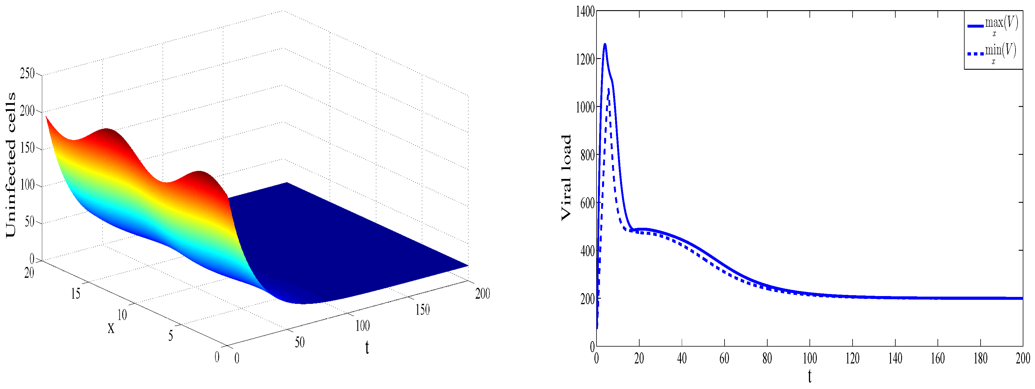
Figure 1 shows spatiotemporal dynamics of uninfected cells (left) and the maximal and the minimal values of the virus concentration in space as a function of time (right). For the values of parameters considered in this example, the basic reproduction number R 0 = 0.22 < 1 , which implies that the virus-free equilibrium is stable. Therefore, as expected, solution converges toward the equilibrium E f = ( 8.27 × 10 2 , 0 , 0 , 0 , 0 ) .
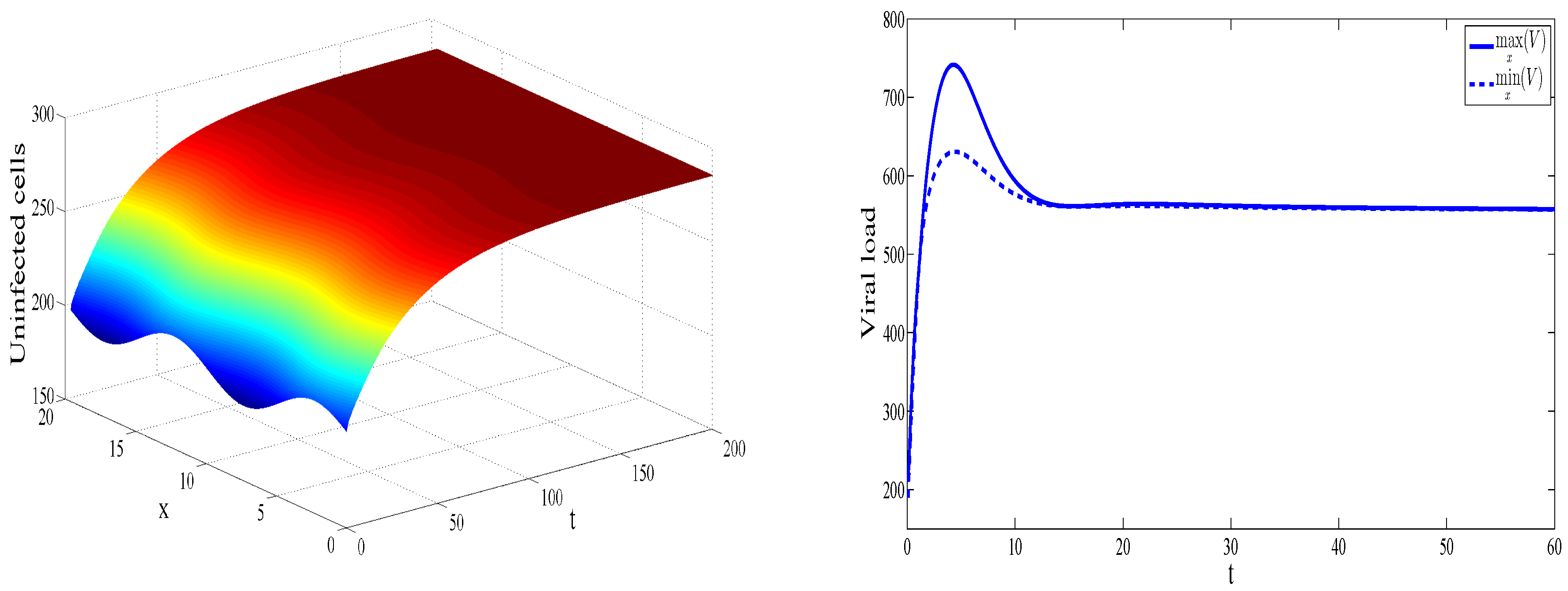
To illustrate convergence to the endemic equilibrium point E 1 , we considered the values of parameters presented in Figure 2. In this case, the basic reproduction number is greater than 1, R 0 = 11.05 > 1 , and the immune reproduction number is less than 1, R C T L = 3.596 × 10 1 < 1 . Therefore, the free-immune endemic equilibrium E 1 = ( 19.96 , 5.98 × 10 1 , 1.14 , 199.78 , 0 ) is globally stable.
In the case considered in Figure 3, we obtain R 0 = 11.05 > 1 and R C T L = 4.13 > 1 . Consequently, we observe that the endemic equilibrium E 2 = ( 285.12 , 6.55 , 3.33 , 555.55 , 660.86 ) is stable. This, numerical results support the theoretical findings.

5. Discussion and Conclusions

In this work, we study a model of viral infection in the presence of CTL cells and latently infected cells. We take into consideration not only the variation in time, but also spatial variation of virus distribution and its diffusion, where uninfected cells, latently infected cells, infected cells, and CTL cells do not exhibit any such spatial mobility. As a result, we show the stability of the free-disease equilibrium using the construction of a Lyapunov function when the reproduction number is less than one ( R 0 < 1 ) . If R 0 > 1 , then two scenarios are established. If R C T L < 1 , then the equilibrium point E 1 is globally asymptotically stable, while, for R C T L > 1 , the equilibrium point E 2 is globally asymptotically stable. We also performed numerical simulations of our model to illustrate behavior of solutions and to confirm the theoretical results. It was established that spatial diffusion of free viruses has no effect on the stability of the steady states. However, the effect appears only for the first days of infection observation.

Author Contributions

All authors contributed equally to this work. All authors have read and agreed to the published version of the manuscript.

Funding

This research was funded by Centre National de la Recherche Scientifique, grant number PICS 244832.

Acknowledgments

The work was partially supported by the France–Morocco program PICS 244832, “RUDN University Program 5-100” and the French–Russian project PRC2307.

Conflicts of Interest

The authors declare no conflict of interest.

Appendix A. The Values of Parameters Used in the Numerical Simulations

The values of parameters used in the numerical simulations are given in Table A1:
Table A1. The values, units and meaning of all used parameters.
ParametersUnitsMeaningValueReferences
λ cells μ L 1 day 1 Source rate of CD4+ T cells [ 0 , 10 ] [27]
k 1 μ L virion 1 day 1 Average of infection [ 2.5 × 10 4 , 0.5 ] [12]
d 1 day 1 Decay rate of healthy cells 0.0139 [12]
d 2 day 1 Death rate of exposed CD4+ T cells 0.0495 [12]
k 2 day 1 The rate that exposed cells become infected CD4+ T cells 1.1 [12]
d 3 day 1 Death rate of infected CD4+ T cells, not by CTL killing 0.5776 [12]
aday 1 The rate of production the virus by infected CD4+ T cells [ 2 , 1250 ] [12]
d 4 day 1 Clearance rate of virus [ 0.3466 , 2.4 ] [12]
p μ L cell 1 day 1 Clearance rate of infection 0.0024 [28]
ccells cell 1 day 1 Activation rate CTL cells 0.15 [28]
bday 1 Death rate of CTL cells 0.5 [28]
dmm 2 day 1 Diffusion coefficient 0.01

References

  1. Perelson, A.S.; Neumann, A.U.; Markowitz, M.; Leonard, J.M.; Ho, D.D. HIV-1 dynamics in vivo: Virion clearance rate, infected cell life-span, and viral generation time. Science 1996, 271, 1582–1586. [Google Scholar] [CrossRef] [Green Version]
  2. Adams, B.M.; Banks, H.T.; Davidian, M.; Kwon, H.D.; Tran, H.T.; Wynne, S.N.; Rosenberg, E.S. HIV dynamics: Modeling, data analysis, and optimal treatment protocols. J. Comput. Appl. Math. 2005, 184, 10–49. [Google Scholar] [CrossRef] [Green Version]
  3. Burchell, A.N.; Winer, R.L.; de Sanjosé, S.; Franco, E.L. Epidemiology and transmission dynamics of genital HPV infection. Vaccine 2006, 24, S52–S61. [Google Scholar] [CrossRef]
  4. Elbasha, E.H.; Dasbach, E.J.; Insinga, R.P. A multi-type HPV transmission model. Bull. Math. Biol. 2008, 70, 2126–2176. [Google Scholar] [CrossRef] [PubMed]
  5. Li, M.; Zu, J. The review of differential equation models of HBV infection dynamics. J. Virol. Methods 2019, 266, 103–113. [Google Scholar] [CrossRef]
  6. Meskaf, A.; Allali, K.; Tabit, Y. Optimal control of a delayed hepatitis B viral infection model with cytotoxic T-lymphocyte and antibody responses. Int. J. Dyn. Control. 2017, 5, 893–902. [Google Scholar] [CrossRef]
  7. Wodarz, D. Hepatitis C virus dynamics and pathology: The role of CTL and antibody responses. J. Gen. Virol. 2003, 84, 1743–1750. [Google Scholar] [CrossRef] [PubMed]
  8. Layden, J.E.; Layden, T.J. How can mathematics help us understand HCV? Gastroenterology 2001, 120, 1546–1549. [Google Scholar] [CrossRef]
  9. Nowak, M.A.; Bangham, C.R.M. Population dynamics of immune responses to persistent viruses. Science 1996, 272, 74–79. [Google Scholar] [CrossRef] [Green Version]
  10. Sun, Q.; Min, L.; Kuang, Y. Global stability of infection-free state and endemic infection state of a modified human immunodeficiency virus infection model. IET Syst. Biol. 2015, 9, 95–103. [Google Scholar] [CrossRef] [Green Version]
  11. Sun, Q.; Min, L. Dynamics Analysis and Simulation of a Modified HIV Infection Model with a Saturated Infection Rate. Comput. Math. Methods Med. 2014. [Google Scholar] [CrossRef] [PubMed]
  12. Allali, K.; Danane, J.; Kuang, Y. Global Analysis for an HIV Infection Model with CTL Immune Response and Infected Cells in Eclipse Phase. Appl. Sci. 2017, 7, 861. [Google Scholar] [CrossRef] [Green Version]
  13. Smith, H.L.; De Leenheer, P. Virus dynamics: A global analysis. SIAM J. Appl. Math. 2003, 63, 1313–1327. [Google Scholar] [CrossRef]
  14. Daar, E.S.; Moudgil, T.; Meyer, R.D.; Ho, D.D. Transient highlevels of viremia in patients with primary human immunodeficiency virus type 1. N. Engl. J. Med. 1991, 324, 961–964. [Google Scholar] [CrossRef] [PubMed]
  15. Kahn, J.O.; Walker, B.D. Acute human immunodeficiency virus type 1 infection. N. Engl. J. Med. 1998, 339, 33–39. [Google Scholar] [CrossRef] [PubMed]
  16. Bocharov, G.; Volpert, V.; Ludewig, B.; Meyerhans, A. Mathematical Immunology of Virus Infections; Springer International Publishing: Cham, Switzerland, 2018. [Google Scholar] [CrossRef]
  17. Kaufmann, G.R.; Cunningham, P.; Kelleher, A.D.; Zauders, J.; Carr, A.; Vizzard, J.; Law, M.; Cooper, D.A. The Sydney Primary HIV Infection Study Group. Patterns of viral dynamics during primary human immunodeficiency virus type 1 infection. J. Infect. Dis. 1998, 178, 1812–1815. [Google Scholar] [CrossRef]
  18. Schacker, T.; Collier, A.; Hughes, J.; Shea, T.; Corey, L. Clinical and epidemiologic features of primary HIV infection. Ann. Int. Med. 1996, 125, 257–264. [Google Scholar] [CrossRef]
  19. Britton, N.F. Essential Mathematical Biology; Springer: London, UK, 2003. [Google Scholar]
  20. Grebennikov, D.; Bouchnita, A.; Volpert, V.; Bessonov, N.; Meyerhans, A.; Bocharov, G. Spatial lymphocyte dynamics in lymph nodes predicts the CTL frequency needed for HIV infection control. Front. Immunol. 2019, 10, 1213. [Google Scholar] [CrossRef]
  21. Maziane, M.; Hattaf, K.; Yousfi, N. Dynamics of a class of HIV infection models with cure of infected cells in eclipse stage. Acta Biotheor. 2015, 63, 363–380. [Google Scholar] [CrossRef]
  22. Hattaf, K.; Yousfi, N. A numerical method for delayed partial differential equations describing infectious diseases. Comput. Math. Appl. 2016, 72, 2741–2750. [Google Scholar] [CrossRef]
  23. Trofimchuk, S.; Volpert, V. Traveling waves for a bistable reaction-diffusion equation with delay. SIAM J. Math. Anal. 2018, 50, 1175–1199. [Google Scholar] [CrossRef] [Green Version]
  24. Bocharov, G.; Meyerhans, A.; Bessonov, N.; Trofimchuk, S.; Volpert, V. Interplay between reaction and diffusion processes in governing the dynamics of virus infections. J. Theor. Biol. 2018, 457, 221–236. [Google Scholar] [CrossRef] [PubMed]
  25. Bessonov, N.; Bocharov, G.; Touaoula, T.M.; Trofimchuk, S.; Volpert, V. Delay reaction-diffusion equation for infection dynamics. Discret. Contin. Dyn. Syst.-B 2019, 24, 2073–2091. [Google Scholar] [CrossRef] [Green Version]
  26. Goudon, T.; Lagoutiere, F.; Tine, L.M. The Lifschitz-Slyozov equation with space-diffusion of monomers. Kinet. Relat. Model. 2012, 5, 325–355. [Google Scholar] [CrossRef]
  27. Wang, Y.; Zhou, Y.; Wu, J.; Heffernan, J. Oscillatory viral dynamics in a delayed HIV pathogenesis model. Math. Biosci. 2009, 219, 104–112. [Google Scholar] [CrossRef]
  28. Zhu, H.; Luo, Y.; Chen, M. Stability and Hopf bifurcation of a HIV infection model with CTL-response delay. Comput. Math. Appl. 2011, 62, 3091–3102. [Google Scholar] [CrossRef] [Green Version]
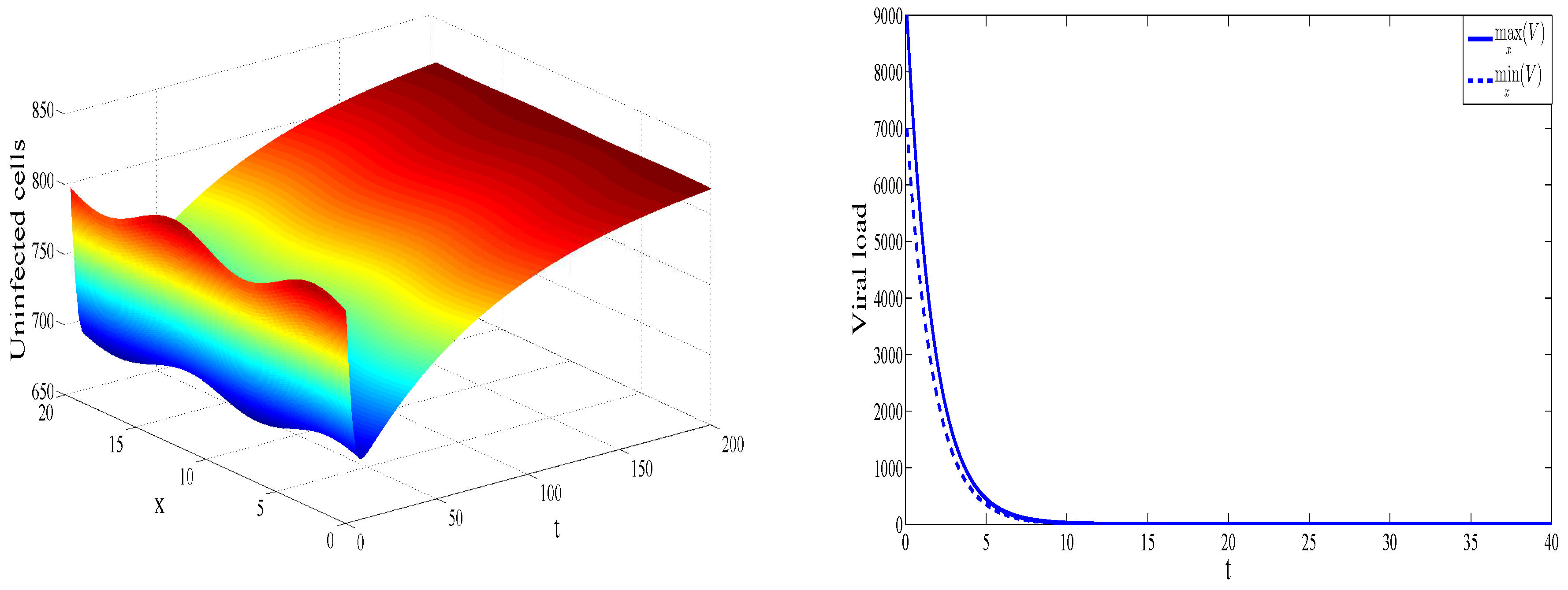
Figure 1. Dynamics of solution for λ = 10 , d 1 = 0.0139 , k 1 = 0.04 , d 2 = 0.0495 , k 2 = 1.1 , d 3 = 0.5776 , a = 2 , d 4 = 0.6 , p = 0.0024 , c = 0.15 , and b = 0.5 . The concentration of uninfected cells is shown as a function of x and t (left). The maximal and the minimal value of the virus concentration with respect to x are shown as functions of time (right).
Mathematics 08 00052 g001
Figure 2. Dynamics of solution for λ = 1 , d 1 = 0.0139 , k 1 = 0.04 , d 2 = 0.0495 , k 2 = 1.1 , d 3 = 0.5776 , a = 100 , d 4 = 0.6 , p = 0.0024 , c = 0.15 , and b = 0.5 . The concentration of uninfected cells is shown as a function of x and t (left). The maximal and the minimal value of the virus concentration with respect to x are shown as functions of time (right).
Mathematics 08 00052 g002
Figure 3. Dynamics of solution for λ = 10 , d 1 = 0.0139 , k 1 = 0.04 , d 2 = 0.0495 , k 2 = 1.1 , d 3 = 0.5776 , a = 100 , d 4 = 0.6 , p = 0.0024 , c = 0.15 , and b = 0.5 . The concentration of uninfected cells is shown as a function of x and t (left). The maximal and the minimal value of the virus concentration with respect to x are shown as functions of time (right).
Mathematics 08 00052 g003
Table 1. The parameters of the mathematical model and their descriptions.
CoefficientDescription
λ The birth rate of the uninfected cells
k 1 The rate of infection
d 1 The natural mortality of the susceptible cells
d 2 The death rate of exposed cells
k 2 The average that exposed cells become infected
d 3 The death rate of infected cells, not by CTL killing
aThe rate of production the virus by infected cells
d 4 The rate of viral clearance
pClearance rate of infection
cActivation rate CTL cells
bDeath rate of CTL cells
dDiffusion coefficient