Stability and Bifurcation of a Delayed Time-Fractional Order Business Cycle Model with a General Liquidity Preference Function and Investment Function

Abstract

In this paper, the business cycle (BC) is described by a delayed time-fractional-order model (DTFOM) with a general liquidity preference function and an investment function. Firstly, the existence and uniqueness of the DTFOM solution are proven. Then, some conditions are presented to guarantee that the positive equilibrium point of DTFOM is locally stable. In addition, Hopf bifurcation is obtained by a new method, where the time delay is regarded as the bifurcation parameter. Finally, a numerical example of DTFOM is given to verify the effectiveness of the proposed model and methods.

1. Introduction

Macroeconomics is an essential economic field that analyzes the general law of economics through macroeconomic indicators such as national income, market investment, and money supply [1]. As one of the most important issues of macroeconomics, business cycle (BC) theory has been studied by many economists because of its realistic meaning and practical value [2].

To obtain the factors involved in fluctuations in the business cycle (BC), many mathematical models are founded on nonlinear dynamics and relative theories that improve the development of BC theory. Using graph analysis, Kaldor [3] proved that a BC exists when the investment and saving function are time-varying nonlinear. Chang and Smyth [4] proved the results shown in [3] by using mathematical theory and gave the conditions required for the existence of limit cycles. J. R.Hicks and A. H. Hansen proposed the IS-LM model, which is an important tool for describing the macroeconomic analysis of the interlinked theoretical structure between the product market and the money market [5]. These early studies are of great significance to current and future BC.

Time delay is a phenomenon existing in practice that often appears in engineering applications [6,7,8]. Time delay is an important factor that also widely exists in economics. Since economics is not only affected by the present state, but also by the past state, the delayed mathematical model is more suitable for describing economic systems, and some significant results have been drawn in recent years [9,10,11]. Considering expectation and delay, Liu and Cai [12] studied a BC model and gave some conditions of stability and bifurcation. Hu and Cao [13,14] studied the Kaldor–Kalecki model of delayed BC. To summarize, time delay is an important reason for fluctuations in BC.

In recent years, the theory of fractional calculus (FC) has not only rapidly developed, but has also been widely applied in many fields [15,16,17,18,19]. In fact, most economic systems have long-term memories. Compared with integer derivatives, since fractional derivatives are related to the entire time domain of the economic process, the fractional-order systems are more suitable for describing economic systems. In the last few years, fractional calculus equations have been widely used to describe a class of economic processes with power law memory and spatial nonlocality. Some continuous-time mathematical models describing economic dynamics with long memory have been proposed [20,21], and some interesting results were obtained. Wang and Huang [22] studied a delayed fractional-order financial system and obtained some conditions of stability and chaos. Ma and Ren [23] studied a fractional-order macroeconomic system and obtained some conditions of stability and Hopf bifurcation. Considering negative parameters, Tacha and Munoz-Pacheco [24] studied a fractional-order finance system, and the cause of chaos was found. Motivated by the above considerations, a new delayed fractional-order model (DFOM) for BC with a general liquidity preference function and an investment function is considered in this paper.

The arrangements of the article are as follows: In Section 2, the model description and some definitions and lemmas are provided. Section 3 shows the main results. The existence and uniqueness of the solution and the local stability and bifurcation of the positive equilibrium point of DFOM for the BC are presented. Numerical simulations and conclusions are respectively presented in Section 4 and Section 5.

2. Preliminaries and Model Descriptions

In this paper, the Caputo form of the fractional-order derivative is used.

Definition 1.

[25] For a continuous function $f\left(t\right)$ and a positive integer n, if $\alpha \in (n-1,n)$ is satisfied, the fractional-order Caputo’s derivative is defined as:

$$D^{\alpha }f\left(t\right)=\frac{1}{\mathsf{\Gamma }(n-\alpha )}{\int }_{t_0}^t\frac{f^{\left(n\right)}\left(\tau \right)}{{(t-\tau )}^{\alpha +1-n}}d\tau ,$$

(1)

where $t_0\in \mathbf{R}$ is the initial time and $\mathsf{\Gamma }(·)$ is the Gamma function.

Definition 2.

[26] For $0<\alpha <1$, under the initial condition $x\left(t_0\right)=x_{t_0}$, $x^{*}$ is called an equilibrium point of system $D^{\alpha }x\left(t\right)=f(t,x)$ if and only if $f(t,x^{*})=0$.

Lemma 1.

[26] For $\alpha \in (0,1]$, under the initial condition $x\left(t_0\right)=x_{t_0}$, if $f(t,x)$ satisfies the local Lipschitz condition, then system $D^{\alpha }x\left(t\right)=f(t,x)$ has a unique solution for $t>t_0$.

Lemma 2.

[27] Suppose that $x^{*}$ is the equilibrium point of system $D^{\alpha }x\left(t\right)=f\left(x\right)$; if $|arg\left({\lambda }_i\right)|>\frac{\alpha \pi }{2}$ is satisfied, then $x^{*}$ is asymptotically locally stable, where ${\lambda }_i$ is any one of the eigenvalues for the Jacobian matrix $J=\partial f/\partial x$ evaluated at $x^{*}$.

We consider the augmented IS-LM BC model given by Gabisch and Lorenz [28],

$$\begin{array}{c}\dot{Y}\left(t\right)=a[I(Y\left(t\right),K\left(t\right),R\left(t\right))-S(Y\left(t\right),R\left(t\right))],\hfill \\ \dot{R}\left(t\right)=b[L(Y\left(t\right),R\left(t\right))-\overline{M}],\hfill \\ \dot{K}\left(t\right)=I(Y\left(t\right),K\left(t\right),R\left(t\right))-\delta K\left(t\right),\hfill \end{array}$$

(2)

where $Y\left(t\right)$, $R\left(t\right)$, and $K\left(t\right)$ represent the gross product, interest rate at time t, and capital stock, respectively. $I\left(Y\right(t),K(t),R(t\left)\right)$ is the investment function, $L\left(Y\right(t),R(t\left)\right)$ is the liquidity preference function, $S\left(Y\right(t),R(t\left)\right)$ is the saving function, and $\overline{M}$ is a constant money supply. $a>0$ and $b>0$ denote the adjustment coefficient of goods and the monetary market, respectively. $0<\delta <1$ represents the depreciation rate of the capital stock.

We consider an investment delay $\tau >0$, which is always encountered in capital stock, and suppose that $S(Y\left(t\right),R\left(t\right))=s_{1}Y\left(t\right)+s_{2}R\left(t\right)$. The DFOM for the BC with a general liquidity preference function and an investment function under the initial conditions $Y\left(\theta \right)={\varphi }_1\left(\theta \right)$, $R\left(\theta \right)={\varphi }_2\left(\theta \right)$, $K\left(\theta \right)={\varphi }_3\left(\theta \right)$ is described as follows:

$$\begin{array}{c}{D}^{\alpha }Y\left(t\right)=a[I(Y\left(t\right),K\left(t\right),R\left(t\right))-s_{1}Y\left(t\right)-s_{2}R\left(t\right)],\hfill \\ D^{\alpha }R\left(t\right)=b[L(Y\left(t\right),R\left(t\right))-\overline{M}],\hfill \\ D^{\alpha }K\left(t\right)=I(Y(t-\tau ),K(t-\tau ),R(t-\tau ))-\delta K\left(t\right),\hfill \end{array}$$

(3)

where $-\tau \le \theta \le 0$, $0<\alpha \le 1$ and $s_1$ and $s_2$ are positive constants.

Suppose that $I\left(Y\right(t),K(t),R(t\left)\right)$, and $L\left(Y\right(t),K(t\left)\right)$ are differentiable. $X\left(t\right)=K(t+\tau )$ is denoted as the expected capital stock. By substituting it into System (3), one obtains:

$$\begin{array}{c}{D}^{\alpha }Y\left(t\right)=a[I(Y\left(t\right),X(t-\tau ),R\left(t\right))-s_{1}Y\left(t\right)-s_{2}R\left(t\right)],\hfill \\ D^{\alpha }R\left(t\right)=b[L(Y\left(t\right),R\left(t\right))-\overline{M}],\hfill \\ D^{\alpha }X\left(t\right)=I(Y\left(t\right),X(t-\tau ),R\left(t\right))-\delta X\left(t\right).\hfill \end{array}$$

(4)

3. Main Results

We firstly prove that the solution of DFOM for BC exists and is unique. In addition, we give some conditions to guarantee that the positive equilibrium point is stable and bifurcates.

3.1. Existence and Uniqueness of the Solution

Theorem 1.

If $C=C([-\tau ,0],{\mathbf{R}}^3)$ is the continuous function of the Banach space and $Z_0\left(t\right)\in C$ is an initial condition, then System (4) has a unique solution $Z\left(t\right)$, where $Z\left(t\right)=\left(Y\right(t),R(t),X(t\left)\right)$.

Proof. 

Consider a mapping $H\left(Z\right)=(H_1\left(Z\right),H_2\left(Z\right),H_3\left(Z\right))$, where:

$$\begin{array}{c}{H}_1\left(Z\left(t\right)\right)=-s_{1}aY\left(t\right)-s_{2}aR\left(t\right)+aI(Y\left(t\right),X(t-\tau ),R\left(t\right)),\hfill \\ H_2\left(Z\left(t\right)\right)=-b\overline{M}+bL(Y\left(t\right),R\left(t\right)),\hfill \\ H_3\left(Z\left(t\right)\right)=-\delta X\left(t\right)+I(Y\left(t\right),X(t-\tau ),R\left(t\right)).\hfill \end{array}$$

(5)

The following conclusion can be made:

$$\begin{array}{cc}\hfill & \parallel H\left(Z\left(t_1\right)\right)-H\left(Z\left(t_2\right)\right)\parallel \hfill \\ \hfill \le & |H_1\left(Z\left(t_1\right)\right)-H_1\left(Z\left(t_2\right)\right)|+|H_2\left(Z\left(t_1\right)\right)-H_2\left(Z\left(t_2\right)\right)|+|H_3\left(Z\left(t_1\right)\right)-H_3\left(Z\left(t_2\right)\right)|\hfill \\ \hfill =& \left|a\right\{[I(Y\left(t_1\right),X(t_1-\tau ),R\left(t_1\right))-I(Y\left(t_2\right),X(t_2-\tau ),R\left(t_2\right))]-s_1[Y\left(t_1\right)-Y\left(t_2\right)]-s_2[R\left(t_1\right)-R\left(t_2\right)]\left\}\right|\hfill \\ \hfill & +|[I(Y\left(t_1\right),X(t_1-\tau ),R\left(t_1\right))-I(Y\left(t_2\right),X(t_2-\tau ),R\left(t_2\right))]-\delta (X\left(t_1\right)-X\left(t_2\right))|\hfill \\ \hfill & +\left|b\right[L(Y\left(t_1\right),R\left(t_1\right))-L(Y\left(t_2\right),R\left(t_2\right))\left]\right|\hfill \\ \hfill \le & |Y\left(t_1\right)-Y\left(t_2\right)\left|\right[a|s_1|+(a+1)|\frac{\partial I(Y\left(T_1\right),X(t_1-\tau ),R\left(t_1\right))}{\partial Y}|+b|\frac{\partial L(Y\left(T_2\right),R\left(t_1\right))}{\partial Y}\left|\right]\hfill \\ \hfill & +max\left\{\right|X(t_1-\tau )-X(t_2-\tau )|,|X\left(t_1\right)-X\left(t_2\right)\left|\right\}\left[\right|(a+1)\frac{\partial I(Y\left(t_2\right),X\left(T_3\right),R\left(t_1\right))}{\partial X}|+\delta ]\hfill \\ \hfill & +|R\left(t_1\right)-R\left(t_2\right)\left|\right[s_2+|(a+1)\frac{\partial I(Y\left(t_2\right),X(t_2-\tau ),R\left(T_4\right))}{\partial R}|+b|\frac{\partial L(Y\left(t_2\right),R\left(T_5\right))}{\partial R}\left|\right]\hfill \\ \hfill & \le L\Vert Z\left(t_1\right)-Z\left(t_2\right)\Vert .\hfill \end{array}$$

(6)

The constants $T_1,T_2,T_4,T_5\in [t_1,t_2]$, $T_3\in [t_1-\tau ,t_2-\tau ]$ exist, satisfying:

$$\begin{array}{cc}\hfill |\frac{\partial I(Y\left(T_1\right),X(t_1-\tau ),R\left(t_1\right))}{\partial Y}|& =\underset{t\in [t_1,t_2]}{max}|\frac{\partial I(Y\left(t\right),X(t_1-\tau ),R\left(t_1\right))}{\partial Y}|,\hfill \\ \hfill |\frac{\partial L(Y\left(T_2\right),R\left(t_1\right))}{\partial Y}|& =\underset{t\in [t_1,t_2]}{max}|\frac{\partial L(Y\left(t\right),R\left(t_1\right))}{\partial Y}|,\hfill \\ \hfill |\frac{\partial I(Y\left(t_2\right),X\left(T_3\right),R\left(t_1\right))}{\partial X}|& =\underset{t\in [t_1-\tau ,t_2-\tau ]}{max}|\frac{\partial I(Y\left(t_2\right),X\left(t\right),R\left(t_1\right))}{\partial X}|,\hfill \\ \hfill |\frac{\partial I(Y\left(t_2\right),X(t_2-\tau ),R\left(T_4\right))}{\partial R}|& =\underset{t\in [t_1,t_2]}{max}|\frac{\partial I(Y\left(t_2\right),X(t_2-\tau ),R\left(t\right))}{\partial R}|,\hfill \\ \hfill |\frac{\partial L(Y\left(t_2\right),R\left(T_5\right))}{\partial R}|& =\underset{t\in [t_1,t_2]}{max}|\frac{\partial L(Y\left(t_2\right),R\left(t\right))}{\partial R}|,\hfill \end{array}$$

(7)

where one chooses a positive constant,

$$\begin{array}{cc}\hfill L=max\{& |s_2|+|(a+1)\frac{\partial I(Y\left(t_2\right),X(t_2-\tau ),R\left(T_3\right))}{\partial R}|+b|\frac{\partial L(Y\left(t_2\right),R\left(T_5\right))}{\partial R}|,\hfill \\ \hfill & |(a+1)\frac{\partial I(Y\left(t_2\right),X\left(T_3\right),R\left(t_1\right))}{\partial X}|+\delta ,\hfill \\ \hfill & a|s_1|+(\alpha +1)|\frac{\partial I(Y\left(T_1\right),X(t_1-\tau ),R\left(t_1\right))}{\partial Y}|+b|\frac{\partial L(Y\left(T_2\right),R\left(t_2\right))}{\partial Y}\left|\right\}.\hfill \end{array}$$

(8)

It is quite clear that $H\left(Z\right)$ satisfies the Lipschitz condition. According to lemma 1, System (4) with $Z_{t_0}$ has a unique solution $Z\left(t\right)$. □

3.2. Stability and Bifurcation

Assume that System (4) contains positive equilibrium points, and let $E^{*}=(Y^{*},R^{*},X^{*})$ be one of them. For convenience, we define:

$$\begin{array}{ccc}\frac{\partial I(Y^{*},X^{*},R^{*})}{Y}=I_Y,\hfill & \frac{\partial L(Y^{*},R^{*})}{Y}=L_Y,\hfill & \hfill \\ \frac{\partial I(Y^{*},X^{*},R^{*})}{R}=I_R,\hfill & \frac{\partial L(Y^{*},R^{*})}{R}=L_R,\hfill & \hfill \\ \frac{\partial I(Y^{*},X^{*},R^{*})}{X}=I_X,\hfill & x\left(t\right)=X\left(t\right)-x^{*},\hfill & \hfill \\ y\left(t\right)=Y\left(t\right)-Y^{*},\hfill & r\left(t\right)=R\left(t\right)-R^{*}\hfill & \hfill .\end{array}$$

(9)

By substituting (9) into (4) and using linearization methods for (4), we get:

$$\begin{array}{c}{D}^{\alpha }y\left(t\right)=a[I_{Y}y\left(t\right)+I_{R}r\left(t\right)+I_{X}x(t-\tau )-s_{1}y\left(t\right)-s_{2}r\left(t\right)],\hfill \\ D^{\alpha }r\left(t\right)=b[L_{Y}y\left(t\right)+L_{R}r\left(t\right)-\overline{M}],\hfill \\ D^{\alpha }x\left(t\right)=I_{Y}y\left(t\right)+I_{R}r\left(t\right)+I_{X}x(t-\tau )-\delta x\left(t\right).\hfill \end{array}$$

(10)

The Jacobian matrix of (10) is described as:

$$J=\left[\begin{array}{ccc}a(I_Y-s_1)& a(I_R-s_2)& a{I}_X{e}^{-s\tau }\\ b{L}_Y& b{L}_R& 0\\ I_Y& I_R& I_X{e}^{-s\tau }-\delta \end{array}\right].$$

Then, the characteristic equation can be expressed as:

$$s^{3\alpha }+a_1{s}^{2\alpha }+a_2{s}^{\alpha }+a_3+(a_4{s}^{2\alpha }+a_5{s}^{\alpha }+a_6)e^{-s\tau }=0,$$

(11)

where:

$$\begin{array}{c}{a}_1=-a(I_Y-s_1)-b{L}_R+\delta ,\hfill \\ a_2=a(I_Y-s_1)(b{L}_R-\delta )-b{L}_R\delta -ab{L}_Y(I_R-s_2),\hfill \\ a_3=ab\delta [(I_Y-s_1)L_R-(I_R-s_2)L_Y],\hfill \\ a_4=I_X,\hfill \\ a_5=a(I_Y-s_1)I_X+b{L}_R{I}_X-a{I}_X{I}_Y,\hfill \\ a_6=-ab(I_Y-s_1)L_R{I}_X-ab{L}_Y{I}_R{I}_X+ab{L}_R{I}_Y{I}_X+ab(I_R-s_2)L_Y{I}_X.\hfill \end{array}$$

(12)

Theorem 2.

For $\tau =0$ and System (4), $E^{*}=(Y^{*},R^{*},X^{*})$ is one of the positive equilibrium points. If the conditions:

(1)

$\Delta \le 0$, $a_1+a_4>0$, $a_2+a_5>0$, $a_3+a_6>0$, and $(a_1+a_4)(a_2+a_5)-(a_3+a_6)>0$,

(2)

$\Delta >0$, $(A+B-\frac{a_1+a_4}{3})<0$, and $|arg(A\omega +B{\omega }^2-\frac{a_1+a_4}{3})|>\frac{\alpha \pi }{2}$,

exist, where $\Delta =\frac{q^2}{4}+\frac{p^3}{27}$, $p=\frac{3(a_2+a_5)-{(a_1+a_4)}^2}{3}$, $q=\frac{2{(a_1+a_4)}^3-9(a_1+a_4)(a_2+a_5)+27(a_3+a_6)}{27}$, $A=\sqrt[3]{-\frac{q}{2}+\sqrt{\frac{q^2}{4}+\frac{p^3}{27}}}$ and $B=\sqrt[3]{-\frac{q}{2}-\sqrt{\frac{q^2}{4}+\frac{p^3}{27}}}$, then $E^{*}$ is locally asymptotically stable.

Proof. 

If $\tau =0$, then (11) can be rewritten as:

$$s^{3\alpha }+(a_1+a_4)s^{2\alpha }+(a_2+a_5)s^{\alpha }+a_3+a_6=0.$$

(13)

Let $s^{\alpha }=\lambda$, and substitute it into (13). This produces:

$${\lambda }^3+(a_1+a_4){\lambda }^2+(a_2+a_5)\lambda +a_3+a_6=0.$$

(14)

Let ${\lambda }^{*}=\lambda +\frac{a_1+a_4}{3}$. Then, (14) can be transformed into:

$${\left({\lambda }^{*}\right)}^3+p{\lambda }^{*}+q=0,$$

(15)

where $p=\frac{3(a_2+a_5)-{(a_1+a_4)}^2}{3}$, $q=\frac{2{(a_1+a_4)}^3-9(a_1+a_4)(a_2+a_5)+27(a_3+a_6)}{27}$.

If $\Delta =\frac{q^2}{4}+\frac{p^3}{27}\le 0$, (15) has three real roots. Thus, (14) has three real roots. Then, according to the Routh–Hurwitz criterion and the theory of the equilibrium point [29,30], if:

$$\begin{array}{c}{a}_2+a_5>0,a_1+a_4>0,a_3+a_6>0,\hfill \\ (a_1+a_4)(a_2+a_5)-(a_3+a_6)>0,\hfill \end{array}$$

(16)

all three real roots are negative. Thus, $|arg\left({\lambda }_i\right)|=\pi >\frac{\alpha \pi }{2}$, and $E^{*}$ is locally asymptotically stable.

If $\Delta =\frac{q^2}{4}+\frac{p^3}{27}>0$, then ${\lambda }_1^{*}=A+B$, ${\lambda }_2^{*}=A\omega +B{\omega }^2$, and ${\lambda }_3^{*}=A{\omega }^2+B\omega$, where $A=\sqrt[3]{-\frac{q}{2}+\sqrt{\frac{q^2}{4}+\frac{p^3}{27}}}$, $B=\sqrt[3]{-\frac{q}{2}-\sqrt{\frac{q^2}{4}+\frac{p^3}{27}}}$, and $\omega =\frac{-1+\sqrt{3}i}{2}$. Thus, ${\lambda }_1=A+B-\frac{a_1+a_4}{3}$, ${\lambda }_2=A\omega +B{\omega }^2-\frac{a_1+a_4}{3}$, and ${\lambda }_3=A{\omega }^2+B\omega -\frac{a_1+a_4}{3}$. If $|arg(A\omega +B{\omega }^2-\frac{a_1+a_4}{3})|>\frac{\alpha \pi }{2}$ and $A+B-\frac{a_1+a_4}{3}<0$, $E^{*}$ is locally asymptotically stable. □

Next, we use the method in [31] to deal with the case where $\tau \ne 0$. Assume that (11) has a purely imaginary root $s=i\phi$$(\phi >0)$ and $a_4{s}^{2\alpha }+a_5{s}^{\alpha }+a_6\ne 0$. By substituting $s=i\phi$ into Equation (11), we get:

$$\begin{array}{c}\hfill a_1{\phi }^{2\alpha }(cos\alpha \pi +sin\left(\alpha \pi \right)i)+a_2{\phi }^{\alpha }(cos\frac{\alpha \pi }{2}+sin\frac{\alpha \pi }{2}i)+a_3+{\phi }^{3\alpha }(cos\frac{3\alpha \pi }{2}+sin\frac{3\alpha \pi }{2}i)\\ \hfill +(a_4{\phi }^{2\alpha }(cos\alpha \pi +isin\alpha \pi )+a_5{\phi }^{\alpha }(cos\frac{\alpha \pi }{2}+isin\frac{\alpha \pi }{2})+a_6)(cos\phi \tau -isin\phi \tau )=0.\end{array}$$

(17)

If we write the real and imaginary parts separately, then we have:

$$\left\{\begin{array}{c}{\phi }^{3\alpha }cos\frac{3\alpha \pi }{2}+a_1{\phi }^{2\alpha }cos\alpha \pi +a_2{\phi }^{\alpha }cos\frac{\alpha \pi }{2}+a_3\hfill \\ =-[a_4{\phi }^{2\alpha }cos(\alpha \pi -\phi \tau )+a_5{\phi }^{\alpha }cos(\frac{\alpha \pi }{2}-\phi \tau )+a_{6}cos\phi \tau ],\hfill \\ {\phi }^{3\alpha }sin\frac{3\alpha \pi }{2}+a_1{\phi }^{2\alpha }sin\alpha \pi +a_2{\phi }^{\alpha }sin\frac{\alpha \pi }{2}\hfill \\ =-[a_4{\phi }^{2\alpha }sin(\alpha \pi -\phi \tau )+a_5{\phi }^{\alpha }sin(\frac{\alpha \pi }{2}-\phi \tau )-a_{6}sin\phi \tau ].\hfill \end{array}\right.$$

(18)

By squaring the corresponding sides of (18) and adding them, we get:

$$\begin{array}{c}{\phi }^{6\alpha }+2a_1\cos \frac{\alpha \pi }{2}{\phi }^{5\alpha }+(a_1^2+2a_{2}cos\alpha \pi -a_4^2){\phi }^{4\alpha }+(2a_{3}cos\frac{3\alpha \pi }{2}+2a_1{a}_{2}cos\frac{\alpha \pi }{2}-2a_4{a}_{5}cos\frac{\alpha \pi }{2}){\phi }^{3\alpha }\hfill \\ +(a_2^2+2a_1{a}_{3}cos\alpha \pi -a_5^2-2a_4{a}_6\cos \alpha \pi ){\phi }^{2\alpha }+(2a_4{a}_{3}cos\frac{\alpha \pi }{2}-2a_5{a}_{6}cos\frac{\alpha \pi }{2}){\phi }^{\alpha }+a_3^2-a_6^2=0.\hfill \end{array}$$

(19)

If we let $h\left(\phi \right)={\phi }^{6\alpha }+2a_1\cos \frac{\alpha \pi }{2}{\phi }^{5\alpha }+(a_1^2+2a_{2}cos\alpha \pi -a_4^2){\phi }^{4\alpha }+(2a_{3}cos\frac{3\alpha \pi }{2}+2a_1{a}_{2}cos\frac{\alpha \pi }{2}-2a_4{a}_{5}cos\frac{\alpha \pi }{2}){\phi }^{3\alpha }+(a_2^2+2a_1{a}_{3}cos\alpha \pi -a_5^2-2a_4{a}_6\cos \alpha \pi ){\phi }^{2\alpha }+(2a_4{a}_{3}cos\frac{\alpha \pi }{2}-2a_5{a}_{6}cos\frac{\alpha \pi }{2}){\phi }^{\alpha }+a_3^2-a_6^2$, and suppose that $a_3^2-a_6^2<0$, then ${\phi }_0$ is one of the positive roots of $h\left(\phi \right)$. Using (17), we get:

$${\tau }_j=\frac{1}{{\phi }_0}\{\arccos -\frac{CE+DF}{E^2+F^2}+2j\pi \},j=0,1,2,\dots ,n,$$

(20)

where:

$$\begin{array}{c}C={\phi }_0^{3\alpha }cos\frac{3\alpha \pi }{2}+a_1{\phi }_0^{2\alpha }cos\alpha \pi +a_2{\phi }_0^{\alpha }cos\frac{\alpha \pi }{2}+a_3,\hfill \\ D={\phi }_0^{3\alpha }sin\frac{3\alpha \pi }{2}+a_1{\phi }_0^{2\alpha }sin\left(\alpha \pi \right)+a_2{\phi }_0^{\alpha }sin\frac{\alpha \pi }{2},\hfill \\ E=a_4{\phi }_0^{2\alpha }cos\alpha \pi +a_5{\phi }_0^{\alpha }cos\frac{\alpha \pi }{2}+a_6,\hfill \\ F=a_4{\phi }_0^{2\alpha }sin\alpha \pi +a_5{\phi }_0^{\alpha }sin\frac{\alpha \pi }{2}.\hfill \end{array}$$

(21)

Then, $\tau$ appears to be a bifurcation parameter. If we assume that (11) has an eigenvalue $\lambda \left(\tau \right)=\omega \left(\tau \right)+i\phi \left(\tau \right)$, then we get $\omega \left({\tau }_0\right)=0$ and $\phi \left({\tau }_0\right)={\phi }_0$, where ${\tau }_0=min\left\{{\tau }_j\right\}$.

Theorem 3.

If we assume that $a_3^2-a_6^2<0$, if $h^{{}^{\prime }}\left({\phi }_0\right)\ne 0$ is satisfied, Hopf bifurcation occurs.

Proof. 

By using the implicit function theorem and differentiating (11) with respect to $\tau$, we get:

$$\frac{ds}{d\tau }=\frac{s{P}_2\left(s\right)e^{-s\tau }}{-\tau P_2\left(s\right)e^{-s\tau }+P_2^{{}^{\prime }}\left(s\right)e^{-s\tau }+P_1^{{}^{\prime }}\left(s\right)},$$

(22)

where $P_1\left(s\right)=s^{3\alpha }+a_1{s}^{2\alpha }+a_2{s}^{\alpha }+a_3$, $P_2\left(s\right)=a_4{s}^{2\alpha }+a_5{s}^{\alpha }+a_6$. Therefore,

$$\begin{array}{cc}\hfill {\frac{ds}{d\tau }}^{-1}=& \frac{-\tau }{s}+\frac{P_2^{{}^{\prime }}\left(s\right)}{s{P}_2\left(s\right)}+\frac{P_1^{{}^{\prime }}\left(s\right)}{s{P}_2\left(s\right)e^{-s\tau }}\hfill \\ \hfill =& \frac{-\tau }{s}+\frac{P_2^{{}^{\prime }}\left(s\right)}{s{P}_2\left(s\right)}-\frac{P_1^{{}^{\prime }}\left(s\right)}{s{P}_1\left(s\right)}.\hfill \end{array}$$

(23)

Then,

$$\begin{array}{cc}\hfill {\left(Re\frac{ds}{d\tau }\right)}^{-1}{|}_{s=i{\phi }_0}=& Re[\frac{P_2^{{}^{\prime }}\left(s\right)}{s{P}_2\left(s\right)}-\frac{P_1^{{}^{\prime }}\left(s\right)}{s{P}_1\left(s\right)}]{|}_{s=i{\phi }_0}\hfill \\ \hfill =& Re[\frac{2\alpha a_4{s}^{2\alpha }+\alpha a_5{s}^{\alpha }}{s^2(a_4{s}^{2\alpha }+a_5{s}^{\alpha }+a_6)}-\frac{3\alpha s^{3\alpha }+2\alpha a_1{s}^{2\alpha }+\alpha a_2{s}^{\alpha }}{s^2(s^{3\alpha }+a_1{s}^{2\alpha }+a_2{s}^{\alpha }+a_3)}]{|}_{s=i{\phi }_0}\hfill \\ \hfill =& \frac{h^{{}^{\prime }}\left({\phi }_0\right)}{2{\phi }_0(a_4^2{\phi }_0^{4\alpha }+2a_4{a}_{5}cos\frac{\alpha \pi }{2}{\phi }_0^{3\alpha }+(a_5^2+2a_4{a}_6)\cos \alpha \pi {\phi }_0^{2\alpha }+2a_5{a}_{6}cos\frac{\alpha \pi }{2}{\phi }_0^{\alpha }+a_6^2)}.\hfill \end{array}$$

(24)

By assuming $a_4{s}^{2\alpha }+a_5{s}^{\alpha }+a_6\ne 0$, we get $2{\phi }_0(a_4^2{\phi }_0^{4\alpha }+2a_4{a}_{5}cos\frac{\alpha \pi }{2}{\phi }_0^{3\alpha }+(a_5^2+2a_4{a}_6)\cos \alpha \pi {\phi }_0^{2\alpha }+2a_5{a}_{6}cos\frac{\alpha \pi }{2}{\phi }_0^{\alpha }+a_6^2)\ne 0$. Thus, if $h^{{}^{\prime }}\left({\phi }_0\right)\ne 0$, $Re\frac{ds}{d\tau }\ne 0$, then the transversality condition holds. Therefore, Hopf bifurcation occurs at $\tau ={\tau }_0$. □

In conclusion, we have the following theorem.

Theorem 4.

If we assume that $a_3^2-a_6^2<0$, $h^{{}^{\prime }}\left({\phi }_0\right)\ne 0$ and the conditions in Theorem 2 are satisfied, we get the following results:

(1)

If $\tau <{\tau }_0$, $E^{*}$ is stable;

(2)

If $\tau >{\tau }_0$, $E^{*}$ is unstable;

(3)

A Hopf bifurcation exists at $\tau ={\tau }_0$.

Remark 1.

According to (20), it is easy to see that ${\tau }_0$ relates to the order α. Therefore, if τ is selected, the order α may be the cause of bifurcation.

4. Numerical Simulation

There are many numerical simulation methods like the Monte Carlo [19] and the predict-evaluate and correct-evaluate (PECE) method [32,33], and the PECE method is used for numerical simulation presented in this section. According to [12], the following Kaldor investment function is used:

$$I(Y\left(t\right),R\left(t\right),K\left(t\right))=\frac{e^{Y\left(t\right)}}{1+e^{Y\left(t\right)}}-cR\left(t\right)-dK\left(t\right),$$

(25)

where $c,d>0$. According to the literature [12,34], the following liquidity preference function is chosen:

$$L(Y\left(t\right),R\left(t\right))=mY\left(t\right)+\frac{n}{R\left(t\right)-\widehat{R}},$$

(26)

where $m,n,\widehat{R}>0$. The following parameter values are chosen:

$$\begin{array}{ccccccc}a=2,\hfill & b=1.5,\hfill & s_1=0.2,\hfill & s_2=0.1,\hfill & c=0.1,\hfill & & d=0.2,\\ m=0.05,\hfill & n=0.0005,\hfill & \widehat{R}=0.001,\hfill & \delta =0.1,\hfill & \overline{M}=0.05,\hfill \end{array}$$

(27)

one can get the following system:

$$\begin{array}{c}{D}^{\alpha }Y\left(t\right)=2[\frac{e^{Y\left(t\right)}}{1+e^{Y\left(t\right)}}-0.1R\left(t\right)-0.2X(t-\tau )-0.2Y\left(t\right)-0.1R\left(t\right)],\hfill \\ D^{\alpha }R\left(t\right)=1.5[0.05Y\left(t\right)+\frac{0.0005}{R\left(t\right)-0.001}-0.05],\hfill \\ D^{\alpha }X\left(t\right)=\frac{e^{Y\left(t\right)}}{1+e^{Y\left(t\right)}}-0.1R\left(t\right)-0.2X(t-\tau )-0.1X\left(t\right).\hfill \end{array}$$

(28)

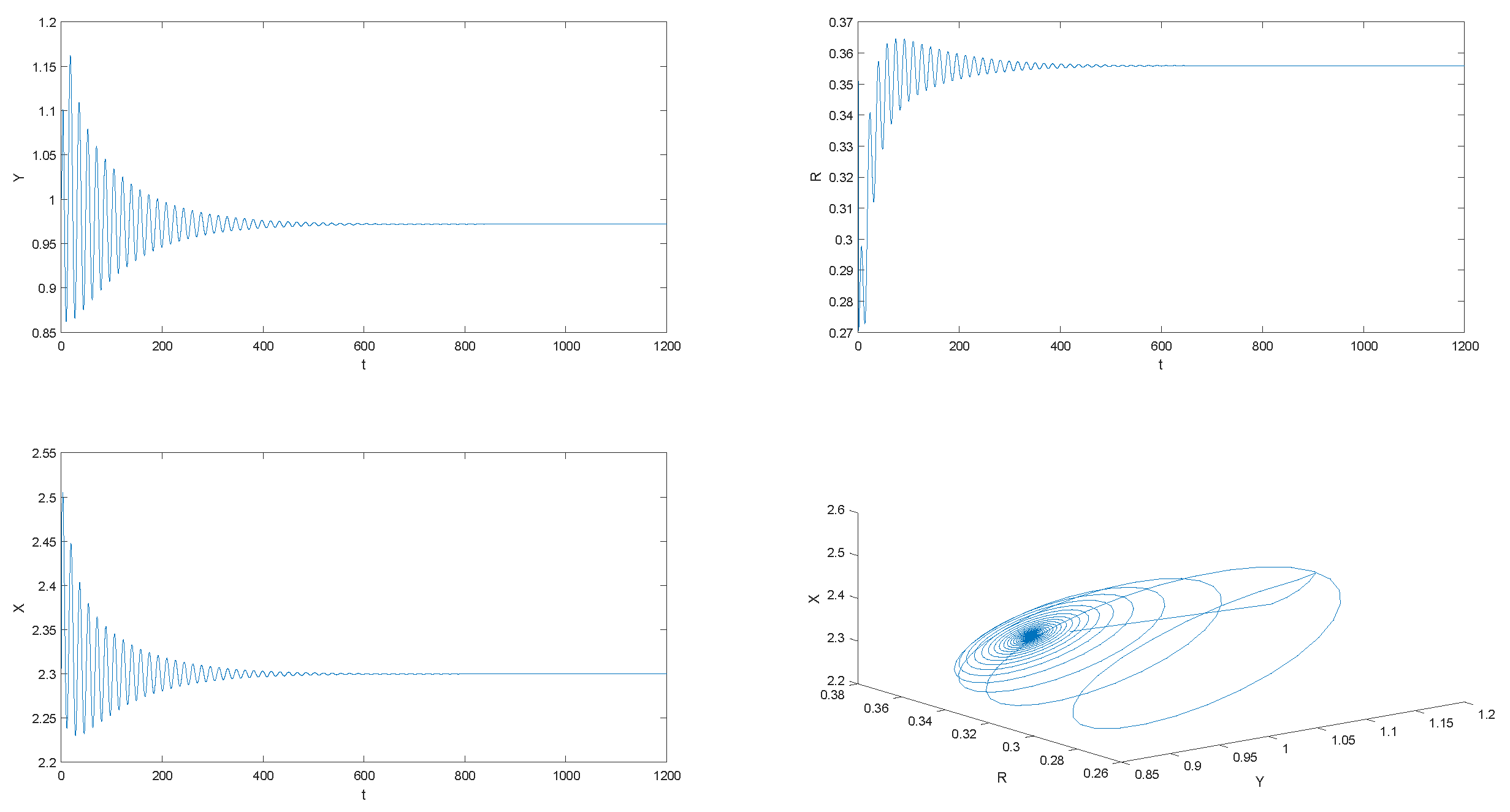
It is easy to see that $E^{*}=(0.97,0.36,2.30)$ is a positive equilibrium point of (28). In this case, $a_3^2-a_6^2<0$, $h^{{}^{\prime }}\left({\phi }_0\right)\ne 0$, and the conditions in Theorem 2 are satisfied. By calculating, the critical value of System (28) is determined to be ${\tau }_0=3.10$ when $\alpha =0.98$. The initial values are chosen to be $Y_0=1$, $R_0=0.35$, and $X\left(\theta \right)=2.3$ where $\theta \in (-\tau ,0)$. This is shown in Figure 1, Figure 2 and Figure 3.

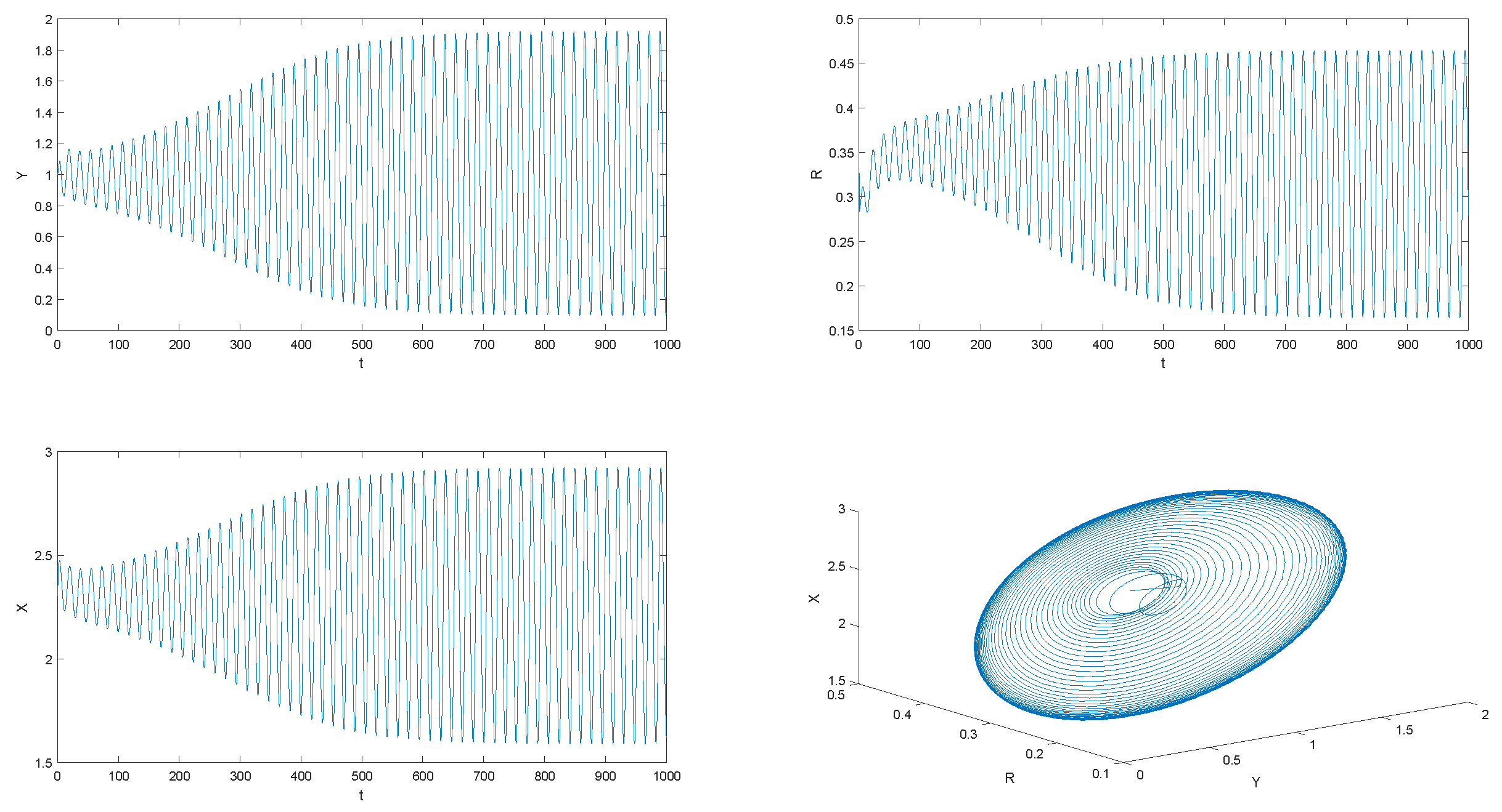
In contrast with the results shown in Figure 1 and Figure 2, if $\tau <{\tau }_0$, $E^{*}$ is stable, and if $\tau >{\tau }_0$, $E^{*}$ is unstable, which conforms to Theorem 4. When comparing Figure 2 and Figure 3, it can be seen that the order $\alpha$ is an important factor in the stability of $E^{*}$ when $\tau$ is selected, which conforms to Remark 1.

By virtue of this important discovery, it can be seen that it is necessary to establish a fractional financial model with an appropriate fractional-order. Moreover, through analyzing the current capital stock, predicting the future capital stock is beneficial to weaken the level of fluctuations.

5. Conclusions

In this paper, a DFOM for BC was established to describe the interaction of markets using the interest rate. The existence and uniqueness of the proposed model were obtained. By mathematical analysis, we found that the investment delay is an important factor in the stability and bifurcation of the economic equilibrium in dynamic macroeconomics. Moreover, we also found that the fractional-order affects the economic equilibrium’s stability and bifurcation.

In order to reduce the factors of macroeconomic instability and to promote stable development, the government can adjust its investment activities from the following aspects, according to the conclusions of this paper. On the one hand, through a series of measures, such as improving the production equipment and working efficiency to reduce investment delay, the economic fluctuations can be weakened. On the other hand, considering the output efficiency of various industries under the current macroeconomic environment, by calculating the average investment delay, the shortage of short-term capital stock in the future can be reasonably predicted, so investment policy and the expected results can be combined to restrain the economic fluctuations caused by investment delay.

References

- Sargent, T.J. Dynamic Macroeconomic Theory; Harvard University Press: Cambridge, MA, USA, 2009. [Google Scholar]
- Goodwin, R.M. The nonlinear accelerator and the persistence of business cycles. Econometrica 1951, 19, 1–17. [Google Scholar] [CrossRef]
- Kaldor, N. A model of the trade cycle. Econ. J. 1940, 50, 78–92. [Google Scholar] [CrossRef]
- Chang, W.W.; Smyth, D.J. The existence and persistence of cycles in a nonlinear model: Kaldor’s 1940 model re-examined. Rev. Econ. Stud. 1971, 38, 37–44. [Google Scholar] [CrossRef]
- Hicks, J.R. Mr. Keynes and the “Classics”: A Suggested Interpretation. Econometrica 1937, 5, 147–159. [Google Scholar] [CrossRef]
- Hu, X.H.; Xia, J.W.; Wei, Y.L.; Meng, B.; Shen, H. Passivity-based state synchronization for semi-Markov jump coupled chaotic neural networks with randomly occurring time delays. Appl. Math. Comput. 2019, 361, 32–41. [Google Scholar] [CrossRef]
- Min, H.F.; Xu, S.Y.; Zhang, B.Y.; Ma, Q. Output-feedback control for stochastic nonlinear systems subject to input saturation and time-varying delay. IEEE Trans. Autom. Control 2019, 64, 359–364. [Google Scholar] [CrossRef]
- Min, H.F.; Xu, S.Y.; Zhang, B.Y.; Ma, Q. Globally adaptive control for stochastic nonlinear time-delay systems with perturbations and its application. Automatica 2019, 102, 105–110. [Google Scholar] [CrossRef]
- Riad, D.; Hattaf, K.; Yousfi, N. Dynamics of a delayed business cycle model with general investment function. Chaos Soliton. Fract. 2016, 85, 110–119. [Google Scholar] [CrossRef]
- Hattaf, K.; Riad, D.; Yousfi, N. A generalized business cycle model with delays in gross product and capital stock. Chaos Soliton. Fract. 2017, 98, 31–37. [Google Scholar] [CrossRef]
- Zhang, X.; Zhu, H. Hopf Bifurcation and Chaos of a Delayed Finance System. Complexity 2019, 6715036. [Google Scholar] [CrossRef]
- Liu, X.; Cai, W.; Lu, J.; Wang, Y. Stability and Hopf bifurcation for a business cycle model with expectation and delay. Commun. Nonlinear Sci. 2015, 25, 149–161. [Google Scholar] [CrossRef]
- Hu, W.; Zhao, H.; Dong, T. Dynamic analysis for a Kaldor-Kalecki model of business cycle with time delay and diffusion effect. Complexity 2018, 4, 1263602. [Google Scholar] [CrossRef]
- Cao, J.Z.; Sun, H.Y. Bifurcation analysis for the Kaldor-Kalecki model with two delays. Adv. Differ. Equ. 2019, 2019, 107. [Google Scholar]
- Fan, Y.; Huang, X.; Wang, Z.; Li, Y. Nonlinear dynamics and chaos in a simplified memristor-based fractional-order neural network with discontinuous memductance function. Nonlinear Dyn. 2018, 9, 1–17. [Google Scholar] [CrossRef]
- Baitiche, Z.; Guerbati, K.; Benchohra, M.; Zhou, Y. Boundary value problems for hybrid Caputo fractional differential equations. Mathematics 2019, 7, 282. [Google Scholar] [CrossRef]
- Secer, A.; Altun, S. A new operational matrix of fractional derivatives to solve systems of fractional differential equations via legendre wavelets. Mathematics 2018, 6, 238. [Google Scholar] [CrossRef]
- Wang, Z.; Xie, Y.; Lu, J.; Li, Y. Stability and bifurcation of a delayed generalized fractional-order prey-predator model with interspecific competition. Appl. Math. Comput. 2019, 347, 360–369. [Google Scholar] [CrossRef]
- Fulger, D.; Scalas, E.; Germano, G. Monte Carlo simulation of uncoupled continuous-time random walks yielding a stochastic solution of the space-time fractional diffusion equation. Phys. Rev. E 2008, 77, 021122. [Google Scholar] [CrossRef] [PubMed]
- Aguilar, J.P.; Korbel, J.; Luchko, Y. Applications of the Fractional Diffusion Equation to Option Pricing and Risk Calculations. Mathematics 2019, 7, 796. [Google Scholar] [CrossRef]
- Tarasov, V.E. Rules for Fractional-Dynamic Generalizations: Difficulties of Constructing Fractional Dynamic Models. Mathematics 2019, 7, 554. [Google Scholar] [CrossRef]
- Wang, Z.; Huang, X.; Shi, G. Analysis of nonlinear dynamics and chaos in a fractional-order financial system with time delay. Comput. Math. Appl. 2011, 62, 1531–1539. [Google Scholar] [CrossRef]
- Ma, J.; Ren, W. Complexity and Hopf bifurcation analysis on a kind of fractional-order IS-LM macroeconomic system. Int. J. Bifurcat. Chaos 2016, 26, 1650181. [Google Scholar] [CrossRef]
- Tacha, O.I.; Munoz-Pacheco, J.M.; Zambrano-Serrano, E.; Stouboulos, I.N.; Pham, V.-T. Determining the chaotic behavior in a fractional-order finance system with negative parameters. Nonlinear Dyn. 2018, 94, 1303–1317. [Google Scholar] [CrossRef]
- Podlubny, I. Fractional Differential Equations; Academic Press: New York, NY, USA, 1999. [Google Scholar]
- Li, Y.; Chen, Y.; Podlubny, I. Stability of fractional-order nonlinear dynamic systems: Lyapunov direct method and generalized Mittag-Leffler stability. Comput. Math. Appl. 2010, 59, 1810–1821. [Google Scholar] [CrossRef]
- Yan, Y.; Kou, C. Stability analysis for a fractional differential model of HIV infection of CD4+ T-cells with time delay. Math. Comput. Simulat. 2012, 82, 1572–1585. [Google Scholar] [CrossRef]
- Gabisch, G.; Lorenz, W.H. Lorenz Business Cycle Theory-a Survey of Methods and Concepts, 2nd ed.; Springer: New York, NY, USA, 1989. [Google Scholar]
- Meng, B. Existence and convergence results of meromorphic solutions to the equilibrium system with angular velocity. Bound. Value Probl. 2019, 2019, 88. [Google Scholar] [CrossRef]
- Meng, B. Minimal thinness with respect to the Schrodinger operator and its applications on singular Schrodinger-type boundary value problems. Bound. Value Probl. 2019, 2019, 91. [Google Scholar] [CrossRef]
- Deng, W.; Li, C.; Lu, J. Stability analysis of linear fractional differential system with multiple time delays. Nonlinear Dyn. 2007, 48, 409–416. [Google Scholar] [CrossRef]
- Wang, Z. A numerical method for delayed fractional-order differential equations. J. Appl. Math. 2013, 2013, 256071. [Google Scholar] [CrossRef]
- Wang, Z.; Huang, X.; Zhou, J. A numerical method for delayed fractional-order differential equations: Based on G-L definition. Appl. Math. Inform. Sci. 2013, 7, 525–529. [Google Scholar] [CrossRef]
- Cesare, D.L.; Sportelli, M. A dynamic IS-LM model with delayed taxation revenues. Chaos Soliton. Fract. 2005, 25, 233–244. [Google Scholar] [CrossRef]
© 2019 by the authors. Licensee MDPI, Basel, Switzerland. This article is an open access article distributed under the terms and conditions of the Creative Commons Attribution (CC BY) license (http://creativecommons.org/licenses/by/4.0/).