Article

Kolmogorov-Arnold-Moser Theory and Symmetries for a Polynomial Quadratic Second Order Difference Equation

by
Tarek F. Ibrahim
1,2 and
Zehra Nurkanović
3,*
1
Department of Mathematics, Faculty of Sciences and Arts in Mahayel Aser, King Khalid University, Abha, Sarat Abida 61914, Saudi Arabia
2
Department of Mathematics, Mansoura University, Mansoura 35516, Egypt
3
Department of Mathematics, University of Tuzla, 75000 Tuzla, Bosnia and Herzegovina
*
Author to whom correspondence should be addressed.
Mathematics 2019, 7(9), 790; https://doi.org/10.3390/math7090790
Submission received: 12 June 2019 / Revised: 1 August 2019 / Accepted: 7 August 2019 / Published: 30 August 2019

Abstract

:
By using the Kolmogorov-Arnold-Moser (KAM) theory, we investigate the stability of two elliptic equilibrium points (zero equilibrium and negative equilibrium) of the difference equation t n + 1 = α t n + β t n 2 t n 1 , n = 0 , 1 , 2 , , where are t 1 , t 0 , α R , α 0 , β > 0 . By using the symmetries we find the periodic solutions with some periods. Finally, some numerical examples are given to verify our theoretical results.

1. Introduction and Preliminaries

In this paper, we investigate the behavior of the polynomial quadratic second order difference equation
t n + 1 = α t n + β t n 2 t n 1 , n = 0 , 1 , 2 , ,
where is parameter β > 0 , parameter α 0 and the initial conditions t 1 , t 0 are real numbers.
In References [1,2] the global dynamics of polynomial difference equations
x n + 1 = c x n 1 2 + d x n 1 + 1 ,
and
x n + 1 = i = 0 3 j = 0 i ζ i j x n i j x n 1 j ,
are studied, where
c > 0 , d > 0 , ζ i j 0 , x 1 0 , x 0 0 n = 0 , 1 , 2 .
In studying the global dynamics of (1) and (2), with non-negative initial conditions and non-negative parameters, the authors used the theory of monotonic maps.
There is extensive literature on polynomial difference equations in the complex domain in the last 30 years by mathematicians. First investigations on polynomial difference equations with non-negative parameters and initial conditions were for a special case
x n + 1 = B x n x n 1 + E x n 1 + F , n = 0 , 1 , 2 , .
This difference equation was the subject of many mathematical results published in papers [3,4,5]. One of open problems in mathematics known as the 16th Hilbert problem is to find the upper limit number of periodic solutions of the system of polynomial differential equations of the forms
d x d t = P ( x , y ) and d y d t = Q ( x , y )
depending on the degree and coefficients of the polynomials P ( x , y ) and Q ( x , y ) , and then determine the local character of periodic solutions. Y. Ilyashenko and J. Écalle ( 1991 / 1992 ) have shown that this number is finite in the case where d e g P = d e g Q = 2 (see [6]).
Equation (1) is a special case of the equation
x n + 1 = i = 0 2 j = 0 i ζ i j x n i j x n 1 j ,
which is equivalent to the following system of difference equations
x n + 1 = i = 0 2 j = 0 i ζ i j x n i j y n j , y n + 1 = x n .
This system is a special case of discrete version of the 16th Hilbert problem and for which, in Reference [7], the authors have shown that under certain conditions may have infinitely many periodic solutions of the period 2, which means that the discrete version of 16th Hilbert problem does not hold.
One of the most famous examples of a polynomial difference equation is the second-order Hénon difference equation
x n + 1 = 1 + B x n 1 A x n 2 , n = 0 , 1 , 2 , .
The dynamics of this equation are very complex, for which the existence of a chaotic attractor has been proven ([8]).
Note that after the substitution
t n = α 2 β α α 4 4 β u n
Equation (1) becomes
α α 4 α 2 u n 2 4 α u n 2 + 4 u n 1 + 4 u n + 1 4 = 0 .
For α 0 and α 4 we get
u n + 1 = 1 α α 4 4 u n 2 u n 1 .
If
a = α α 4 4 , b = 1 ,
we get Hénon’s mapping
u n + 1 = 1 a u n 2 + b u n 1 .
Equation (1) has very specific dynamics. Namely, we cannot find the invariant of this equation and we can use only Kolmogorov-Arnold-Moser (KAM) theory to investigate the dynamics of this equation. Some results about using KAM theory are given in References [9,10,11,12,13,14,15,16,17,18,19,20,21]. Other techniques have been used (not only KAM theory) to study the Lyness’ equation (see References [9,10,11,17,22,23,24,25,26,27]).
The definition of an area preserving map is given in Reference [21] (Definition 1). Also, for the basic results about Birkhoff normal forms and the KAM theory, see References [8,20,21,28,29,30,31] (especially see Theorems 1–4 and Remark 1 in [21]).
Assume that β > 0 . Then Equation (1) has a unique equilibrium t ¯ = 0 for α = 2 and two equilibrium points t ¯ 1 = 0 and t ¯ 2 = 2 α β , where t ¯ 2 is positive for α < 2 and t ¯ 2 is negative for α > 2 .
Equation (1) can be transformed into the system
x n + 1 = β x n 2 + α x n y n y n + 1 = x n .
The map T associated to System (8) takes the form
T x y = β x 2 + α x y x .
Jacobian matrix of map T at the point ( x , y ) is given by
J T x , y = 2 β x + α 1 1 0 .
Since det J T x , y = 1 , the map T is an area preserving map.
Remark 1.
When the equilibrium point of Equation (1) is a non-hyperbolic of elliptic type and T is an area-preserving map, we can apply KAM theory to the investigation of its stability.
Lemma 1.
Assume that β > 0 .
1.
For α , 2 2 , the equilibrium ( 0 , 0 ) is a saddle point.
2.
For α = ± 2 the equilibrium ( 0 , 0 ) is non-hyperbolic of the parabolic type.
3.
For α 2 , 2 the equilibrium ( 0 , 0 ) is non-hyperbolic of the elliptic type.
Proof. 
For x ¯ = y ¯ = 0 , α R , β > 0 :
J 0 = J T 0 , 0 = α 1 1 0 .
The characteristic equation at ( 0 , 0 ) is
λ 2 α λ + 1 = 0 ,
and we have the following cases:
  • λ 1 , 2 = α ± α 2 4 2 for α , 2 2 , , and λ 1 1 , 0 , λ 2 < 1 or λ 1 0 , 1 , λ 2 > 1 ,
  • λ 1 , 2 = 1 for α = 2 and λ 1 , 2 = 1 for α = 2 ,
  • λ 1 , 2 = α ± i 4 α 2 2 for α 2 , 2 .
  □
Lemma 2.
Assume that β > 0 .
1.
For α , 2 the positive equilibrium 2 α β , 2 α β is a saddle point.
2.
For α 2 , 6 the negative equilibrium 2 α β , 2 α β is non-hyperbolic of the elliptic type.
3.
For α = 6 the negative equilibrium 2 α β , 2 α β is non-hyperbolic of the parabolic type.
4.
For α > 6 the negative equilibrium 2 α β , 2 α β is a saddle point.
Proof. 
For x ¯ = y ¯ = 2 α β , α R , β > 0 we have
J T x ¯ , x ¯ = 4 α 1 1 0 .
The corresponding characteristic equation is:
λ 2 + α 4 λ + 1 = 0 .
So that:
  • λ 1 = 4 α α 2 α 6 2 0 , 1 , λ 2 = 4 α + α 2 α 6 2 > 1 for α , 2 .
  • λ 1 , 2 = 4 α ± i α 2 6 α 2 for α 2 , 6 and λ 1 , 2 = 1 .
  • λ 1 , 2 = 1 for α = 6 .
  • λ 1 = 4 α α 2 α 6 2 < 1 , λ 2 = 4 α + α 2 α 6 2 1 , 0 for α > 6 .
  □
This paper is organized as follows. By using KAM theorem, in Section 2, we will prove that the equilibrium points t ¯ 1 = 0 for α ( 2 , 2 ) \ 1 , 1 2 , 0 , β > 0 and t ¯ 1 = 2 α β for α ( 2 , 6 ) \ 4 , 9 2 , 5 , β > 0 are stable. In Section 3, we will prove that there exists an infinite number of periodic solutions. Also, we will study the minimal possible period (M.P.P.) for periodic orbit in the neighborhood of the equilibrium point 0 , 0 for α ( 2 , 2 ) \ 1 , 1 2 , 0 , β > 0 . By using the symmetries, in Section 4, we will find the periodic solutions with some periods and several numerical examples are given.

2. KAM Theory Applied to Equation (1)

Theorem 1.
The equilibrium point t ¯ = 0 of (1) is stable for α ( 2 , 2 ) \ 1 , 1 2 , 0 and β > 0 .
Proof. 
For α 2 , 2 the zero equilibrium is non-hyperbolic of the elliptic type. The characteristic Equation (9) at ( 0 , 0 ) has the roots λ = α + i 4 α 2 2 , λ ¯ = α i 4 α 2 2 . So,
λ 2 = α 2 2 2 + α 4 α 2 2 i , λ 3 = α ( α 2 3 ) 2 + ( α 2 1 ) 4 α 2 2 i ,
and
λ 4 = α 4 4 α 2 + 2 2 + α ( α 2 2 ) 4 α 2 2 i .
Clearly λ = 1 , λ 3 1 , λ 4 1 for α 2 , 1 1 , 0 0 , 2 .
Now, we will find the Birkhoff normal form of System (8) (see Theorem 1 in Reference [21]). The change of variables
x n y n = 1 1 λ ¯ λ u n v n = u n + v n λ ¯ u n + λ v n
transforms System (8) into
u n + 1 = λ u n + σ u n + v n 2 , v n + 1 = λ ¯ v n + σ ¯ u n + v n 2 ,
where
σ = λ β λ λ ¯ .
Also, the change of variables
u n = ξ n + k = 0 2 a 2 k ξ n 2 k η n k + k = 0 3 a 3 k ξ n 3 k η n k
v n = η n + k = 0 2 a 2 k ¯ ξ n k η n 2 k + k = 0 3 a 3 k ¯ ξ n k η n 3 k
reduces System (10) to the form
ξ n + 1 = λ ξ n + α 2 ξ n 2 η n + O 4 , η n + 1 = λ ¯ η n + α 2 ¯ ξ n η n 2 + O 4 ,
where (see Reference [14])
α 2 = 2 a 21 + a 21 ¯ σ + 2 a 20 + a 22 ¯ σ = 4 R e a 21 σ + 2 a 20 + a 22 ¯ σ ,
a 21 = 2 σ 1 λ , a 22 = σ λ ¯ 2 λ ,
σ = β 2 1 i α 4 α 2 .
Furthermore
a 20 + a 22 ¯ = β ( α 2 ) ( α + 1 ) ,
α 2 = σ 4 R e a 21 + 2 a 20 + a 22 ¯ = 2 β ( ( 2 α + 1 ) ) ( 2 α ) ( α + 1 ) σ ,
α 2 = β 2 ( ( 2 α + 1 ) ) ( 2 α ) ( α + 1 ) 1 i α 4 α 2 .
Thus
R e α 2 = β 2 ( ( 2 α + 1 ) ) ( 2 α ) ( α + 1 ) .
By using the transformation
ξ n = r n + i s n ,
η n = r n i s n ,
we obtain (see Theorem 1, for l = 4 , in Reference [21]):
cos γ 0 = R e λ = α 2 1 , 1 for α 2 , 2 ,
γ 1 = R e α 2 sin γ 0 ,
i.e.,
γ 1 = β 2 ( 2 α + 1 ) α + 1 α 2 1 α 2 / 4 .
Since α ( 2 , 2 ) \ 1 , 1 2 , 0 , this implies γ 1 0 .   □
Theorem 2.
The negative equilibrium point t ¯ = 2 α β of (1) is stable for α ( 2 , 6 ) \ 4 , 9 2 , 5 and β > 0 .
Proof. 
For the negative equilibrium t ¯ 2 = 2 α β , α ( 2 , 6 ) , we use the substitution
x n = t n t ¯ 2 = t n 2 α β , y n = x n 1 ,
and Equation (1) can be transformed into the system
x n + 1 = β x n 2 α 4 x n x n 1 , y n + 1 = x n .
The map G associated with System (14) takes the form
G x y = β x 2 α 4 x y x .
We see that
J G x , y = 2 β x α + 4 1 1 0 ,
and det J G x , y = 1 . So, the map G is an area preserving map and we will apply KAM theory to System (14).
Now, for x ¯ = y ¯ = 0 , α 2 , 6 we have
J 0 = J G 0 , 0 = 4 α 1 1 0 .
The corresponding characteristic equation at equilibrium 0 , 0 is:
λ 2 + α 4 λ + 1 = 0 ,
from which
λ = 4 α + i α 2 6 α 2 , λ ¯ = 4 α i α 2 6 α 2 ,
λ = λ ¯ = 1 ,
λ 2 = 8 α + α 2 + 14 2 + 4 α i α 2 6 α 2 , λ 3 = α 4 8 α + α 2 + 13 2 + i α 5 α 3 α 2 6 α 2 ,
λ 4 = 224 α + 92 α 2 16 α 3 + α 4 + 194 2 α 4 8 α + α 2 + 14 α 2 6 α 2 i .
Clearly λ = 1 , λ 3 1 , λ 4 1 for α 2 , 4 4 , 5 5 , 6 .
Now, the change of variables
x n y n = 1 1 λ ¯ λ u n v n = u n + v n λ ¯ u n + λ v n
transforms System (14) into System (10), where
σ = λ β λ λ ¯ .
Now, for α 2 , 4 4 , 5 5 , 6 we obtain
σ = β 2 1 + α 4 α 2 6 α i ,
and
α 2 = 2 β 2 α 9 α 2 α 5 β 2 1 + α 4 α 2 6 α i .
Thus
R e α 2 = β 2 2 α 9 α 2 α 5 .
Now, we obtain
cos γ 0 = R e λ = 4 α 2 1 , 1 for α 2 , 6 ,
γ 1 = R e α 2 sin γ 0 ,
i.e.,
γ 1 = 2 β 2 2 α 9 α 2 α 5 α 2 6 α .
This implies that γ 1 0 for α ( 2 , 6 ) \ 4 , 9 2 , 5 and β > 0 .   □
For the bifurcation diagrams (B.D.) which indicate the appearance of chaos see Figure 1, Figure 2, Figure 3 and Figure 4.

3. Periodic Points and Orbits

In this section, we study the M.P.P. for a periodic orbit in the neighborhood of the equilibrium ( 0 , 0 ) where α 2 , 1 1 , 1 2 1 2 , 0 0 , 2 and β > 0 .
Lemma 3.
M.P.P. for a periodic orbit in the neighborhood of the elliptic equilibrium ( 0 , 0 ) is 3.
Proof. 
The eigenvalues at the elliptic equilibrium are of the form λ = e ± i ϕ with c o s ( ϕ ) = α 2 , 0 < ϕ < π . Then the period of the motion around the equilibrium must be q > 2 π ϕ > 2 . So, the map T cannot have an orbit of period less than 3 in a neighborhood of the elliptic equilibrium ( 0 , 0 ) .   □
For example, if α = 0.5 , then 2 π / ϕ 4.7668 . So M.P.P. is 5 . If α = 1.5 , then 2 π / ϕ 8.6936 and M.P.P. is 9 . Figure 5 visualize M.P.P. as a function of parameter α . Figure 6 gives us some possible orbits (S.P.O.) around the elliptic equilibrium ( 0 , 0 ) for α = 0.5 and β = 1.5 and Figure 7 gives us S.P.O. around the elliptic equilibrium ( 1 , 1 ) for α = 3.5 and β = 1.5 .
Remark 2.
Equation (1) has the period-three solutions
, α α 2 4 α 4 2 β , α α 2 4 α 4 2 β , α + 2 α 2 4 α 4 2 β , ,
and
, α + α 2 4 α 4 2 β , α + α 2 4 α 4 2 β , α + 2 + α 2 4 α 4 2 β , ,
for
α , 2 2 2 2 + 2 2 , + .
See Figure 5.
Remark 3.
Notice that Equation (1) has a minimal period-two solution
, α + 2 α + 2 α 6 2 β , α + 2 + α + 2 α 6 2 β ,
for
α , 2 6 , + .
The Jacobian matrix of the map T 2 in the minimal period-two solutions is
J T 2 = α 2 + 4 α + 15 2 ± α 2 4 α 12 2 ± α + 2 α 6 1 ,
with the eigenvalues:
λ 1 , 2 = 1 2 α 2 + 2 α + 7 ± 1 2 α 6 α + 2 4 α + α 2 16 .
So, the minimal period-two solution is
1.
a saddle point for α , 2 2 5 2 + 2 5 , + ,
2.
non-hyperbolic of the parabolic type for α = 2 ± 2 5 ,
3.
non-hyperbolic of the elliptic type for
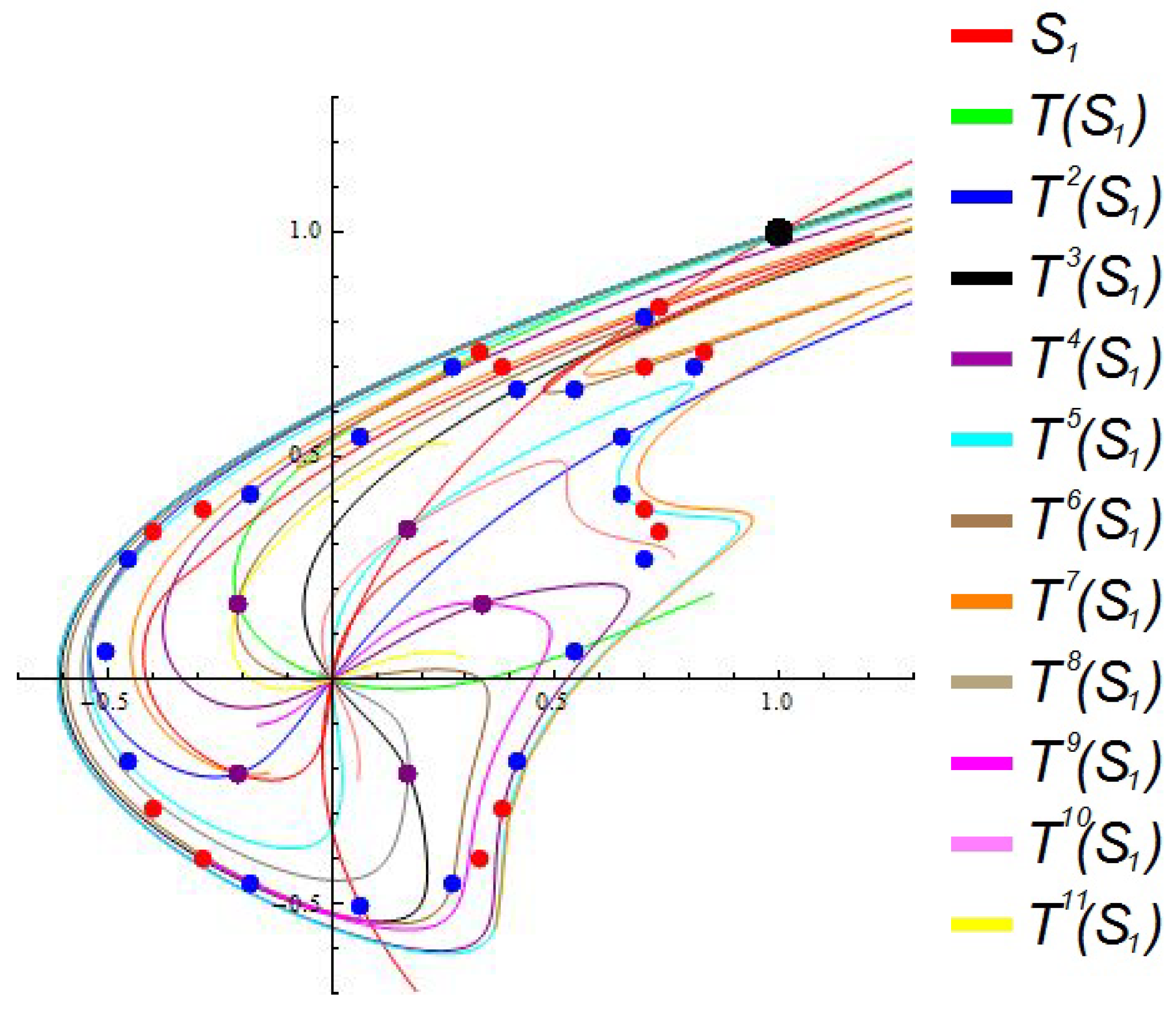
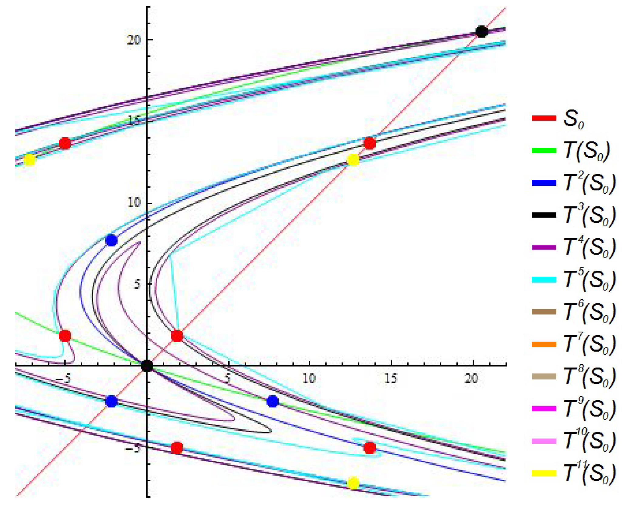
 α 2 2 5 , 2 6 , 2 + 2 5 .

4. Symmetries

It is well known that symmetries play an important role because they have special dynamic behavior. See References [12,28] and Theorem 13 in Reference [13]. Now, the map T associated with the system (8) can be rewritten as follows:
T ( x , y ) = ( β x 2 + α x y , x ) ,
and
T 1 ( x , y ) = ( y , β y 2 + α y x ) .
The involution R ( x , y ) = y , x is a reversor for the map T. Indeed,
( R T R ) ( x , y ) = ( R T ) y , x = R β y 2 + α y x , y = ( y , β y 2 + α y x ) = T 1 ( x , y ) .
Thus T = I 1 I 0 where I 0 ( x , y ) = R ( x , y ) = ( y , x ) and
I 1 ( x , y ) = T R ( x , y ) = β y 2 + α y x , y .
The symmetry lines corresponding to I 0 and I 1 are
S 0 = { ( x , y ) : x = y } , S 1 = { ( x , y ) : ( α + β y ) y = 2 x } .
Periodic orbits on the symmetry line S 0 with even period n are searched for by starting with points ( x 0 , x 0 ) S 0 and imposing that ( x n / 2 , y n / 2 ) S 0 , where
( x n / 2 , y n / 2 ) = T n / 2 ( x 0 , x 0 ) .
This reduces to a one-dimensional root finding for the equation x n / 2 = y n / 2 , where the unknown is x 0 . Also, periodic orbits on S 0 with odd period n are obtained by solving for x 0 the equation y ( n + 1 ) / 2 ( α + β y ( n + 1 ) / 2 ) = 2 x ( n + 1 ) / 2 where
( x ( n + 1 ) / 2 , y ( n + 1 ) / 2 ) = T ( n + 1 ) / 2 ( x 0 , x 0 ) .
Visualization of some periodic orbits can be seen in Figure 8, Figure 9, Figure 10, Figure 11, Figure 12 and Figure 13. For example, in Figure 8, for α = 0.5 we have cyan points
( x 1 , y 1 ) = 0.5235660872586801 , 0.5235660872586801 S 0 S 16 ,
( x 2 , y 2 ) = 0.5060816278767843 , 0.2564826010712121 S 4 S 20 ,
( x 3 , y 3 ) = 0.2564826010712121 , 0.27916534036279644 S 2 S 18 ,
where S 16 = T 8 ( S 0 ) , S 4 = T 2 ( S 0 ) , S 20 = T 10 ( S 0 ) , S 2 = T ( S 0 ) , S 18 = T 9 ( S 0 ) , and then
T 16 0 ( x 1 , y 1 ) = T 16 ( x 1 , y 1 ) = ( x 1 , y 1 ) ,
T 20 4 ( x 2 , y 2 ) = T 16 ( x 2 , y 2 ) = ( x 2 , y 2 ) ,
T 18 2 ( x 3 , y 3 ) = T 16 ( x 3 , y 3 ) = ( x 3 , y 3 ) .
Also, for α = 2.1 , in Figure 10, we have red point
( x , y ) = 13.671359641163505 , 5 . S 4 S 10 ,
where S 4 = T 2 ( S 0 ) , S 10 = T 5 ( S 0 ) , and then
T 10 4 ( x , y ) = T 6 ( x , y ) = ( x , y ) .
Remark 4.
All Figures are generated by Dynamica 3 [8].

5. Conclusions

By using KAM theory, under certain conditions on parameter α , we proved the stability of the zero equilibrium and the negative equilibrium of the difference Equation (1). Also, by using symmetries we proved the existence of periodic solutions with certain periods.

Author Contributions

Both authors have contributed equally and significantly to the contents of this paper.

Funding

This research was funded by a Deanship of scientific research in King Khalid University under grant number GRP-324-40 and by FMON Bosnia and Herzegovina grant number 01/2-5240-1/18.

Acknowledgments

The authors are grateful to two anonymous referees for a number of helpful and constructive suggestions, which improved the presentation of results.

Conflicts of Interest

The authors declare no conflict of interest.

References

  1. Bektešević, J.; Kulenović, M.R.S.; Pilav, E. Global dynamics of quadratic second order difference equation in the first quadrant. Appl. Math. Comput. 2014, 227, 50–65. [Google Scholar] [CrossRef]
  2. Bektešević, J.; Kulenović, M.R.S.; Pilav, E. Asymptotic approximations of a stable and unstable manifolds of a two-dimensional quadratic map. J. Comp. Anal. Appl. 2016, 21, 35–51. [Google Scholar]
  3. Bedford, E. Complex Hénon maps with semi-parabolic fixed points. J. Differ. Equ. Appl. 2010, 16, 425–426. [Google Scholar] [CrossRef]
  4. Bedford, E.; Smillie, J. Real polynomial diffeomorphisms with maximal entropy: Tangencies. Ann. Math. 2004, 160, 1–26. [Google Scholar] [CrossRef] [Green Version]
  5. Milnor, J. Dynamics in One Complex Variable. (AM-160), 3rd ed.; Princeton University Press: Princenton, NJ, USA; Oxford, UK, 2011; p. 160. ISBN 9781400835539. [Google Scholar]
  6. Ilyashenko, Y. Centennial history of Hilbert’s 16th problem. Bull. Am. Math. Soc. (N.S.) 2002, 39, 301–354. [Google Scholar] [CrossRef]
  7. Bektešević, J.; Kulenović, M.R.S.; Pilav, E. Global dynamics of cubic second order difference equation in the first quadrant. Adv. Differ. Equ. 2015, 176, 2015. [Google Scholar] [CrossRef]
  8. Kulenović, M.R.S.; Merino, O. Discrete Dynamical Systems and Difference Equations with Mathematica; Chapman and Hall/CRC: Boca Raton, FL, USA; London, UK, 2002. [Google Scholar]
  9. Bastien, G.; Rogalski, M. On the algebraic difference equations un+2un = ψ(un+1) in ℝ+, related to a family of elliptic quartics in the plane. Adv. Differ. Equ. 2005, 3, 227–261. [Google Scholar] [CrossRef]
  10. Bastien, G.; Rogalski, M. On the algebraic difference equations un+2 + un = ψ(un+1) in ℝ, related to a family of elliptic quartics in the plane. J. Math. Anal. Appl. 2007, 326, 822–844. [Google Scholar] [CrossRef]
  11. Cima, A.; Gasull, A.; Mańosa, V. Dynamics of rational discrete dynamical systems via first integrals. Int. J. Bifur. Chaos Appl. Sci. Eng. 2006, 16, 631–645. [Google Scholar] [CrossRef]
  12. Del-Castillo-Negrete, D.; Greene, J.M.; Morrison, E.J. Area preserving nontwist maps: periodic orbits and transition to chaos. Physica D 1996, 91, 1–23. [Google Scholar] [CrossRef]
  13. Garić-Demirović, M.; Nurkanović, M.; Nurkanović, Z. Stability, periodicity and symmetries of certain second-order fractional difference equation with quadratic terms via KAM theory. Math. Methods Appl. Sci. 2017, 40, 306–318. [Google Scholar] [CrossRef]
  14. Hrustić, S.J.; Kulenović, M.R.S.; Nurkanović, Z.; Pilav, E. Birkhoff normal forms, KAM theory and symmetries for certain second order rational difference equation with quadratic term. Int. J. Differ. Equ. 2015, 10, 181–199. [Google Scholar]
  15. Janowski, E.J.; Kulenović, M.R.S.; Nurkanović, Z. Stability of the k-th Order Lyness’ Equation with a Period-k Coefficient. Int. J. Bifur. Chaos Appl. Sci. Eng. 2007, 17, 143–152. [Google Scholar] [CrossRef]
  16. Kulenović, M.R.S. Invariants and related Liapunov functions for difference equations. Appl. Math. Lett. 2000, 13, 1–8. [Google Scholar] [CrossRef] [Green Version]
  17. Kulenović, M.R.S.; Nurkanović, Z. Stability of Lyness’ Equation with Period-three Coeffcient. Rad. Mat. 2004, 12, 153–161. [Google Scholar]
  18. Kulenović, M.R.S.; Nurkanović, Z. Stability of Lyness’ Equation with Period-two Coeficient via KAM Theory. J. Concr. Appl. Math. 2008, 6, 229–245. [Google Scholar]
  19. Kulenović, M.R.S.; Nurkanović, Z.; Pilav, E. Birkhoff Normal Forms and KAM Theory for Gumowski-Mira Equation. Sci. World J. 2014, 2014, 819290. [Google Scholar] [CrossRef] [PubMed]
  20. Ladas, G.; Tzanetopoulos, G.; Tovbis, A. On May’s host parasitoid model. J. Differ. Equ. Appl. 1996, 2, 195–204. [Google Scholar] [CrossRef]
  21. Nurkanović, M.; Nurkanović, Z. Birkhoff Normal Forms, KAM Theory, periodicity and symmetries for certain rational difference equation with cubic terms. Sarajevo J. Math. 2016, 12, 217–231. [Google Scholar] [CrossRef]
  22. Beukers, F.; Cushman, R. Zeeman’s monotonicity conjecture. J. Differ. Equ. 1998, 143, 191–200. [Google Scholar] [CrossRef]
  23. Cima, A.; Gasull, A.; Mańosa, V. Non-autonomous two-periodic Gumowski-Mira difference equation. Int. J. Bifur. Chaos Appl. Sci. Eng. 2012, 16, 14. [Google Scholar]
  24. Cima, A.; Gasull, A.; Mańosa, V. Non-integrability of measure preserving maps via Lie symmetries. arxiv 2015, arXiv:1503.05348. [Google Scholar] [CrossRef]
  25. Clark, C.A.; Janowski, E.J.; Kulenović, M.R.S. Stability of the Gumowski-Mira equation with period-two coefficient. J. Math. Anal. Appl. 2005, 307, 292–304. [Google Scholar] [CrossRef]
  26. Kocic, V.L.; Ladas, G.; Tzanetopoulos, G.; Thomas, E. On the stability of Lyness’ equation. Dynam. Contin. Discrete Impuls. Syst. 1995, 1, 245–254. [Google Scholar]
  27. Zeeman, E.C. Geometric Unfolding of a Difference Equation; Preprint; Hertford College: Oxford, UK, 1996. [Google Scholar]
  28. Gidea, M.; Meiss, J.D.; Ugarcovici, I.; Weiss, H. Applications of KAM theory to population dynamics. J. Biol. Dyn. 2011, 5, 44–63. [Google Scholar] [CrossRef] [Green Version]
  29. Hale, J.K.; Kocak, H. Dynamics and Bifurcation; Springer: New York, NY, USA, 1991. [Google Scholar]
  30. Papaschinopoulos, G.; Schinas, C.J. Stability of a class of nonlinear difference equations. J. Math. Anal. Appl. 1999, 230, 211–222. [Google Scholar] [CrossRef]
  31. Tabor, M. Chaos and Integrability in Nonlinear Dynamics: An Introduction; A Wiley-Interscience Publication, John Wiley and Sons, Inc.: New York, NY, USA, 1989. [Google Scholar]
Figure 1. B.D. in ( β x ) —plane, β between 0.8 and 1.6 , α = 0.5 and the initial conditions ( 0.2 , 035 ) .
Mathematics 07 00790 g001
Figure 2. B.D. in ( α x ) —plane, α between 0.45 and 0.55 , β = 1.5 and the initial conditions ( 0.2 , 0.35 ) .
Mathematics 07 00790 g002
Figure 3. B.D. in ( β x ) —plane, β between 0.4 and 0.5 , α = 1.9 and the initial conditions ( 0.1 , 0.2 ) .
Mathematics 07 00790 g003
Figure 4. B.D. in ( β x ) —plane, β between 0.15 and 0.215 , α = 2.1 and the initial conditions ( 0.1 , 0.2 ) .
Mathematics 07 00790 g004
Figure 5. Minimal possible period (M.P.P.) as a function of parameter α .
Mathematics 07 00790 g005
Figure 6. Some possible orbit (S.P.O.) around the elliptic equilibrium ( 0 , 0 ) for α = 0.5 and β = 1.5 .
Mathematics 07 00790 g006
Figure 7. S.P.O. around the elliptic equilibrium ( 1 , 1 ) for α = 3.5 and β = 1.5 .
Mathematics 07 00790 g007
Figure 8. Possible orbit (P.O.) of period 5—Blue, 14—Red, 16—Cyan and Green, 17 and 18—Black for α = 0.5 .
Mathematics 07 00790 g008
Figure 9. Period 5—Purple, 13—Red and 18—Blue for α = 0.5 (see Table 1).
Mathematics 07 00790 g009
Figure 10. Period 3—Yellow and Blue and period 6—Red for α = 2.1 (see Table 2).
Mathematics 07 00790 g010
Figure 11. Period 5 for α = 0.5 , t(−1) = 0.3387353751757066‘, t(0) = 0.1707400845904967‘ (see Table 1).
Mathematics 07 00790 g011
Figure 12. Period 13 for α = 0.5 , t(−1) = 0.8334938164207883‘, t(0) = 0.7294074106139652‘ (see Table 1).
Mathematics 07 00790 g012
Figure 13. Period 18 for α = 0.5 t(−1) = 0.812543579771728’, t(0) = 0.6983061967141229’ (see Table 1).
Mathematics 07 00790 g013
Table 1. List of periodical solutions of the period 5,13,14,16 and 18 for α = 0.5 , β = 1.5 .
PSolution
5 { ( 0.20963706815151129 , 0.20963706815150332 ) ,
( 0.33873537517570756 , 0.17074008459048975 ) , ( 0.17074008459048975 , 0.20963706815151129 ) ,
( 0.1707400845904967 , 0.3387353751757066 ) , ( 0.20963706815150332 , 0.1707400845904967 ) }
13 { ( 0.7294074106139652 , 0.8334938164207883 ) , ( 0.32926264487404866 , 0.7294074106139652 ) ,
( 0.40215525421276 , 0.32926264487404866 ) , ( 0.28774699924403424 , 0.40215525421276 ) ,
( 0.38247925795166227 , 0.28774699924403424 ) , ( 0.6984222023647466 , 0.38247925795166227 ) ,
( 0.6984222023647456 , 0.6984222023647466 ) , ( 0.38247925795165866 , 0.6984222023647456 ) ,
( 0.2877469992440391 , 0.38247925795165866 ) , ( 0.833493816420777 , 0.7294074106139614 ) ,
( 0.32926264487404977 , 0.40215525421275455 ) , ( 0.7294074106139614 , 0.32926264487404977 ) ,
( 0.40215525421275455 , 0.2877469992440391 ) }
14 { ( 0.7089960985742474 , 0.7089960985742474 ) , ( 0.3995151524031322 , 0.7089960985742474 ) ,
( 0.2698199868731344 , 0.3995151524031322 ) , ( 0.4252209078653717 , 0.2698199868731344 ) ,
( 0.32842876366922497 , 0.4252209078653717 ) , ( 0.7512334689079276 , 0.32842876366922497 ) ,
( 0.8937155579958962 , 0.7512334689079276 ) , ( 0.8937155579958947 , 0.8937155579958962 ) ,
( 0.7512334689079214 , 0.8937155579958947 ) , ( 0.32842876366920937 , 0.7512334689079214 ) ,
( 0.4252209078653887 , 0.32842876366920937 ) , ( 0.26981998687310554 , 0.4252209078653887 ) ,
( 0.39951515240314023 , 0.26981998687310554 ) , ( 0.7089960985742323 , 0.39951515240314023 ) }
16 { ( 0.5235660872586801 , 0.5235660872586801 ) , ( 0.1493991279617058 , 0.5235660872586801 ) ,
( 0.41538637412425006 , 0.1493991279617058 ) , ( 0.09827355531169368 , 0.41538637412425006 ) ,
( 0.380736133978804 , 0.09827355531169368 ) , ( 0.5060816278767843 , 0.380736133978804 ) ,
( 0.2564826010712122 , 0.5060816278767843 ) , ( 0.2791653403627964 , 0.2564826010712122 ) ,
( 0.27916534036279644 , 0.2791653403627964 ) , ( 0.2564826010712121 , 0.27916534036279644 ) ,
( 0.5060816278767843 , 0.2564826010712121 ) , ( 0.38073613397880407 , 0.5060816278767843 ) ,
( 0.09827355531169357 , 0.38073613397880407 ) , ( 0.4153863741242501 , 0.09827355531169357 ) ,
( 0.14939912796170576 , 0.4153863741242501 ) , ( 0.5235660872586801 , 0.14939912796170576 ) }
18 { ( 0.6983061967141229 , 0.812543579771728 ) , ( 0.2680568351393483 , 0.6983061967141229 ) ,
( 0.456496078847063 , 0.2680568351393483 ) , ( 0.1837218695587639 , 0.456496078847063 ) ,
( 0.41526573209893225 , 0.1837218695587639 ) , ( 0.6500231779917233 , 0.41526573209893225 ) ,
( 0.5435410547866188 , 0.6500231779917233 ) , ( 0.06490266675941142 , 0.5435410547866188 ) ,
( 0.5047711871781883 , 0.06490266675941142 ) , ( 0.06490266675941075 , 0.5047711871781883 ) ,
( 0.5435410547866183 , 0.06490266675941075 ) , ( 0.6500231779917228 , 0.5435410547866183 ) ,
( 0.41526573209893164 , 0.6500231779917228 ) , ( 0.18372186955876452 , 0.41526573209893164 ) ,
( 0.45649607884706234 , 0.18372186955876452 ) , ( 0.6983061967141223 , 0.2680568351393484 ) ,
( 0.2680568351393484 , 0.45649607884706234 ) , ( 0.8125435797717264 , 0.6983061967141223 ) }
Table 2. List of periodical solutions of the period 2,3,6,14 and 18 for α = 2.1 , β = 0.2 .
PSolution
2 { ( 2.0 , 2.5 ) , ( 2.5 , 2.0 ) }
3 { ( 2.170411039827144 , 2.170411039827144 ) , ( 7.6670411039824855 , 2.170411039827144 ) ,
( 2.1704110398316487 , 7.6670411039824855 ) }
3 { ( 12.670411039841001 , 12.670411039841001 ) , ( 2.170411039827144 , 12.670411039841001 ) ,
( 12.670411039841001 , 2.170411039827144 ) }
6 { ( 1.8286403588364943 , 1.8286403588364943 ) , ( 5 . , 1.8286403588364943 ) ,
( 13.671359641163505 , 5 . ) , ( 13.671359641163505 , 13.671359641163505 ) ,
( 5 . , 13.671359641163505 ) , ( 1.8286403588364948 , 5 . ) }
14 { ( 1.5939516328297656 , 1.8407502773040598 ) , ( 2.0146845131985835 , 1.5939516328297656 ) ,
( 1.825095107342817 , 2.0146845131985835 ) , ( 2.4842096423906703 , 1.825095107342817 ) ,
( 2.1574856322082345 , 2.4842096423906703 ) , ( 2.9774590358836153 , 2.1574856322082345 ) ,
( 2.32212588107436 , 2.9774590358836153 ) , ( 2.9774590358836153 , 2.32212588107436 ) ,
( 2.1574856322082345 , 2.9774590358836153 ) , ( 2.4842096423906703 , 2.1574856322082345 ) ,
( 1.8250951073428172 , 2.4842096423906703 ) , ( 2.014684513198584 , 1.8250951073428172 ) ,
( 1.5939516328297665 , 2.014684513198584 ) , ( 1.8407502773040616 , 1.5939516328297665 ) }
18 { ( 0.7387370612506275 , 0.7583266606426369 ) , ( 0.9021676571167236 , 0.7387370612506275 ) ,
( 0.9930337223849965 , 0.9021676571167236 ) , ( 1.3804263546505298 , 0.9930337223849965 ) ,
( 1.5247462382583659 , 1.3804263546505298 ) , ( 2.286510963908646 , 1.5247462382583659 ) ,
( 2.2313003083349026 , 2.286510963908646 ) , ( 3.394959896789736 , 2.2313003083349026 ) ,
( 2.592964934761428 , 3.394959896789736 ) , ( 3.3949598967897314 , 2.592964934761428 ) ,
( 2.2313003083348995 , 3.3949598967897314 ) , ( 2.2865109639086407 , 2.2313003083348995 ) ,
( 1.524746238258362 , 2.2865109639086407 ) , ( 1.380426354650525 , 1.524746238258362 ) ,
( 0.9930337223849932 , 1.380426354650525 ) , ( 0.90216765711672 , 0.9930337223849932 ) ,
( 0.7387370612506245 , 0.90216765711672 ) , ( 0.7583266606426334 , 0.7387370612506245 ) }

