Abstract
Brazil is an important player when it comes to biofuel and agricultural production. The knowledge of the price relationship between these markets has increasing importance. This paper adopts several tools, namely the Bai–Perron test of breakpoints, the Johansen cointegration test and the vector error correction model exploited by the orthogonal impulse response and the forecast error variance decomposition, for investigating the price transmission among the ethanol and the main Brazil’s agricultural commodities (sugar, cotton, arabica coffee, robusta coffee, live cattle, corn and soybean). The data series cover the period from January 2011 up to December 2018. The results suggest a stronger price transmission from the ethanol commodity to the agricultural commodities, rather than the opposite situation.
1. Introduction
Since the beginning of the 21st century Brazil is a reference in the biofuel production, with particular emphasises in the ethanol commodity. The Brazilian ethanol production began growing in the 1970’s, and continued increasing while the oil prices were significantly rising in the London and New York stock exchanges in the mid of 2000’s. Following this trend, the USA advanced in the ethanol production from corn that was subsequently approved by the Energy Policy of Act, or simply, the Energy Bill, in mid 2005 [1].
Those efforts boosted the USA ethanol production to overcome that of Brazilian in 2006. However, that same year was marked by an important discovery in the history of the Brazilian fuel market. Indeed, the pre-salt layer located in the Santos basin, on the southeastern coast of Brazil, was detected and became one of the most prolific petroleum systems in the world. In a short time after the findings, considerable investments in the oil sector start occurred and, the gasoline production gained the attention of government, companies and investors, resulting in a cutting off on the ethanol investment. As a consequence, after an initial surge of 76 ethanol plants constructed in the period 2007–2010, at least 26 ethanol plants were shut down during 2011–2014, on the state of Sao Paulo [2].
One of the strategies of Brazil’s sugarcane crop season for 2011–2012 was the commercial compromise with the USA. The deal included the exportation of Brazil’s ethanol from sugarcane to the USA since that guaranteed a premium for this biofuel [3]. On the other hand, Brazil imported corn-based ethanol from the USA, due to a sugarcane crop shortfall that resulted in an increase of the biofuel prices for consumers.
A strategy for recovering the ethanol production in 2011–2012 included the reduction of taxes for the ethanol sector and the increased amount of ethanol in the blend with gasoline, going from 20% to 25%. [4]. Simultaneously, the government offered to sugarcane producers interest-free subsidized loans in order to recover the earlier production state. This strategy brought results to the sector, since in the crop season of 2014 the ethanol production reached a record of 28.6 billion liters [5]. However, this also reflected by lowering the prices of sugar in the international market, which is usually the alternative option when producing ethanol from plants. A third strategy was to control the fuel prices in the internal market, which was later proved to be the reason for inadequate conditions in the market competition [6]. Indeed, by avoiding (artificially) the gasoline prices to fluctuate relative to the international market prices, lower costs for ethanol in the domestic market were forced, guaranteeing competitivity vis a vis the values spent with gasoline [7].
The following years (2015–2017) brought instability to the sector, since Brazil faced an economic recession and, besides, a presidential impeachment process took place leading not only to a lower consumption of ethanol in the internal market, but also to a decrease of light vehicles sales and unemployment [8,9].
In recent years, the Brazilian energy sector is recovering, and an optimistic scenario emerged, where the internal prices are again linked to those of the international market. Furthermore, a new investment cycle was recently announced for the sector until 2030, in the scope of the Renovabio program [10]. Also, the current mandatory blending of ethanol in gasoline reached 27%, but with a perspective of increasing to 30% by 2022 and 40% by 2030 [11].
Brazil is also an important player when it comes to agricultural commodities [12,13]. The country is recognized as one of the major exporters of agricultural products, primarily as a result of its strong performance in the sector. According to the Food and Agriculture Organization of the United Nations (FAO), Brazilian agriculture products contributed to about 4% of the country’s gross domestic product (GDP) [FAO Statistical Yearbook 2016, http://www.fao.org/faostat/en/, acessed June 17, 2019]. In fact, one can see exported products influencing this margin, such as the sugarcane and its derivatives (ethanol and sugar), soybean, coffee, beef, orange juice, and corn. Most of these products are negotiated in the Brazilian Stock Exchange, B3 S.A. It is important to highlight that the country’s agricultural area is increasing each year, requiring, therefore, agricultural machinery and equipment that lead to a significant impact on the energy expenditure.
The price volatility of the Brazilian ethanol is primarily influenced by the following market factors [14]: (i) the amount of sugarcane production; (ii) the percentage of sugarcane available for the production of ethanol; (iii) the consumer income; (iv) the number of the light commercial fleet vehicles; and (v) the price of the gasoline, directly influencing the ethanol prices in result to the blend of the two fuels.
Janda and Kristoufek [11] reviewed the literature in the scope of time series analysis of price transmission from food to energy commodities and vice versa. They concluded that, due to policy-induced trade barriers, there is not sufficient evidence of an integrated international biofuel market, including major producers, such as the US, European and Brazilian markets. Fowowe [15], Reboredo [16], Nazlioglu and Soytas [17] found some weak and almost neutral price transmission between the agricultural commodities and the energy prices. On the other hand, for different agricultural commodities, time periods and regions, several researchers [18,19,20,21,22,23,24,25,26,27,28,29,30,31,32,33,34] found significant evidences that the crude oil prices influence those commodities, such as for the cases of the soybean, corn, wheat, rice and sugar. Similarly, several of other studies [35,36,37,38,39,40,41,42,43,44] explored the ethanol relationship with agricultural commodities. It was found that, in general, ethanol prices dynamics are affected by sugar prices in Brazil. Besides, Capitani et al. [37] verified that there is weak linkage between the ethanol and the international prices.
The standard approach in most of these studies requires analyzing a plethora of variables. The need to understand the relationships between a large number of variables makes multivariate analysis a laborious task due to the sheer bulk of data. Indeed, all variables are considered simultaneously and their effects are not interpreted separately. In turn, bivariate analysis allows the association, correlation and analysis of two variables and, if properly applied, provides solid and useful information. One should note that is not sufficient to observe a set of variables and to apply multivariate techniques, because, if they are not linked together, one has to the bivariate analysis to obtain more significative information.
Several researchers applied different tools and concepts such as, error correction models (ECM), vector error correction models (VECM) and cointegration for studying the agricultural and energy commodities [8,9,15,24,33,34,36,43,44,45,46,47,48,49,50,51,52,53,54,55,56,57,58,59,60,61,62,63,64,65,66,67,68]. Mattos et al. [9] discussed the price transmission for the future markets of agricultural commodities using VECM. They evaluated the impact on the price transmission in the futures prices of the Chicago Mercantile Exchange and the Brazilian Stock Exchange in the spot prices of the corn in the Brazilian internal market. Mallory et al. [62] explored the topic and analyzed long-term relations between the ethanol, corn and natural gas in the USA.
The main goal of this work is to investigate the bilateral price relationship between the Brazilian ethanol (ETH) and each one of the major Brazilian agricultural commodities. For this purpose, we adopt several mathematical tools, namely the Bai-Perron test of structural changes, the Johansen cointegration test and the bivariate VECM exploited by the orthogonal impulse response (OIR) and the forecast error variance decomposition (FEVD).
2. Data and Methodology
We consider the spot prices of the ETH and seven important commodities in the Brazilian agricultural GDP, such as the sugar (SUG), cotton (COT), live cattle (LCA), Arabica coffee (ARA), Robusta coffee (ROB), corn (COR) and soybean (SOY). The work aims to measure the impact of ethanol prices against agricultural commodities and vice versa. Such evaluation is possible using multivariate models that are described in the follow-up of this paper.
The data were obtained from the Center for Advanced Studies on Applied Economics/University of Sao Paulo (CEPEA/USP) and the CEPEA methodology for the daily pricing of these products can be found in its website www.cepea.esalq.usp.br. We adopt daily spot prices TS for the ethanol and the seven agricultural commodities for a time interval between January 2011 and December 2018.
Bearing in mind that during this period many changes occurred in the Brazilian energy sector, we evaluate the presence of breakpoints in the prices of the ethanol TS by means of the Bai–Perron algorithm [69]. The main idea consists in obtaining the optimal number b of breakpoints in the TS using an information criterion, namely the Bayesian information criterion (BIC).
The Bai–Perron algorithm is a dynamic method that estimates multiple structural changes (i.e., breakpoints) as global minimizers of the residual sum of squares in a given TS [69]. This technique tests the deviations from stability in the linear regression model by assuming the existence of b breakpoints, and that the coefficients vary from one regression to the other. Therefore, we have time sub-intervals and each i-th regression model can be described as [69,70,71]
where the index i represents the time interval index for intervals, is the observed independent variable, is the vector of coefficients, and stands for the disturbance. Therefore, the algorithm estimates the breakpoints by minimizing the residual sum of squares of the equation. The estimated breakpoint values of the ethanol TS are listed in Table 1 for five tested options (denoted A to E).

Table 1.
The Bayesian information criterion (BIC) criterion, Bai–Perron test and the corresponding breakpoints options (A–E) in the daily ethanol time series (TS) based on the Center for Advanced Studies on Applied Economics/University of Sao Paulo (CEPEA) methodology.
As stated in [69], the Schwarz criterion, or simply the BIC, was applied for structural break inference by Yao [72]. The BIC value is defined as , where is the log-likelihood of the model, k is the number of independent parameters and m is the number of the TS values (e.g., the number of samples). Thus, the criterion represents the statistics that maximizes the chance of identifying the best fitting model to the TS. Then, the model with the lowest BIC value is chosen as the best model [73]. This is commonly applied for selecting the model dimension by estimating the number of breaks. Therefore, for the ethanol TS breakpoints, we obtained from the algorithm five possible options A-E, where A and E are the minimum and maximum values corresponding to one BP and five BP, respectively. The BIC values and the estimated b values are listed in Table 1.
From Table 1 we verify that is the optimal number of breakpoints in the TS since the BIC shows a slightly lower value. By other words, leads to the best fitting and involves five sub-periods denoted as to in the follow-up. Therefore, we have: (i) from January/2011 to May/2012, (ii) from May/2012 to November/2013, (iii) from November/2013 to September/2015, (iv) from September/2015 to October/2017, and (v) from October/2017 to December/2018. The TS of the eight commodities and the corresponding sub-periods are illustrated in Figure 1.
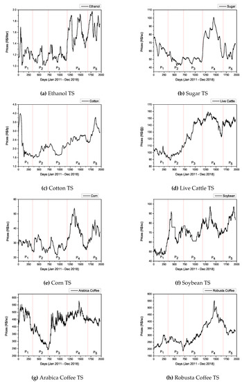
Figure 1.
Spot prices time series (TS) of the eight commodities and the corresponding sub-periods to .
Costa and Burnquist [74] listed different factors that help to understand the four breakpoints in option D. Concerning , we observe a peak price for the ethanol at the beginning of this period. After, the price tends to reduce pointing the first breakpoint found. During the price is maintaining lower than at the beginning of achieving the lowest price at the end of the . This was due to the price control politics in the energy sector of Brazil influencing directly the ethanol prices. Besides, the gradual decreasing of the so-called “Contribution of Intervention in the Economic Domain tax” for gasoline, completely removed at the end of 2012, also affected the ethanol price that became less competitive in the domestic market. Nonetheless, in the final of the price increased again leading to another breakpoint. The sub-period ended in September of 2015 when the ethanol prices were skyrocketing due to the corruption scandals in Brazil’s energy state firm Petrobras that affected the whole sector and produced another breakpoint. The last breakpoint is due to the new pricing policy adopted by Petrobras in the sector. For this reason, ethanol prices may again fluctuate more freely in the internal market.
2.1. Cointegration of Time Series
The cointegration relation between two TS was firstly introduced by Granger [75]. Later, Engle and Granger [76] explored an error correction model. A simple way for explaining a cointegration relation was proposed by Murray [77] under the title “the metaphor of the drunk and her dog”. In order to investigate the price transmission process among the ethanol and other agricultural commodities, the cointegration hypothesis is considered. The process of adjustment was pointed by Murray [77] as the error correction model.
For non-stationary TS, the distance between two series can be stationary, since the adjustment occurs for each step. In this case, the TS are said to be cointegrated of order zero. For a cointegration process to be presented in two TS, both must have the same integration order n, where n is the number of times that a non-stationary TS needs to be differentiate in order to become stationary [77]. Therefore, considering the error correction terms c and d one can write
where t stands for the discrete-time sampling instants, and are the cointegrated variables, and are the white noise stationary steps and is the cointegration relation between the variables x and y.
Aaron Smith and Robin Harrison [78] formulated an extension of the original metaphor by exploring the multiple cointegration with 3 or more cointegrated variables, with the work entitled “A drunk, her dog and a boyfriend: an illustration of multiple cointegration and error correction”.
Often, we observe some confusion between the terms “cointegration” and “correlation”. Alexander [79] points that a cointegration process takes into account both the concepts of integration and stationarity, while that is not considered in a correlation measure. Additionally, the correlation calculates a linear association between two TS. The cointegration of two or more TS can be studied, while a correlation is simply a coefficient in the range []. However, a cointegration process cannot be quantified, since, instead, it is identified.
In this work, we evaluate the cointegration process among the 7 agricultural commodities prices, namely the sugar, cotton, live cattle, corn, soybean, Arabica coffee and Robusta coffee, with respect to the ethanol prices. The cointegration is calculated using the Johansen test, and the VECM model is estimated when the cointegration between a particular commodity with respect to the ethanol is verified.
The Johansen Test for Cointegration
Johansen [80] proposed a statistical test to determine the cointegration relation between two TS. It is known that the cointegration process is directly linked to the VECM since the test is based on the matrix coefficients and that compose the model. The parameters are related to the long-run equilibrium. The parameters (so-called “speed adjustment parameters”) are related to how fast the series tends to return the equilibrium after some perturbation. We can determine how many steps are required for the series to come back to the equilibrium by using the relation .
The Johansen test [81,82] is applied to verify if the rank (r) of the matrix is equal to zero (null hypothesis). If this implicates a the non-existence of the error correction term (ECT). Otherwise, if , then the null hypothesis is rejected and there is a cointegration relation between the analyzed TS. Johansen proposed two possibles tests, namely, the Max-Eigen and the Trace tests, that are based on the assumption of a pure unit root. In contrast to the method for cointegration validation of Engle-Granger [76], the test purposed by Johansen allows the study of more than one cointegration relation among the variables. For this reason, the Johansen test was applied in this work in view of analyzing possible cointegration processes involving the prices of agricultural commodities versus the ethanol.
2.2. The Vector Error Correction Model
The ECM was introduced by Sargan [83]. Later the idea was employed by Davidson [84], evolving toward the VECM methodology. The VECM is based on the generalized vector autoregression (VAR), that allows an adjustment of a regression model between multiple variables to evaluate its relationship.
Let us consider and as two non-cointegrated and stationary TS. Then, the approach from the VAR(j) model is possible as [85,86]
where and are the equation autoregressive terms of and , respectively, and and denote white-noise disturbances. On the other hand, if the TS were not initialy stationary, then we had the VAR(j) in the differences given by [85,86]:
If a cointegration process was found among two or more TS, then the ECT can be implemented and the VAR model becomes a VECM. Note that for implementing the VECM it was not needed that both TS are stationary. Indeed, once the values are calculated from the ECT modeling they are adjusted, so that a stationary ECT is returned, and then applied in the regression equation. Thus, the ECT is expressed in the VECM as , for each price equation, where represents the equilibrium equation between the prices. A VECM is expressed as [9,46,87,88]
3. Results and Discussion
In this section, the results for the cointegration test are presented and discussed. Moreover, the VECM model is estimated for the cointegrated pairs by means of the VECM equation, OIR and FEVD. Section 3.1 analyses the results of the Johansen test in the different sub-periods. Section 3.2 discusses the VECM results adjusted for the sub-periods where the cointegration process occurs, that is, where a price transmission between the ethanol and the agricultural commodities, and vice versa, was found.
3.1. Cointegration from Johansen Test
The Johansen test is applied based on the max-migen and trace tests as mentioned Section 2.1. The cointegration process is evaluated for the full period (2011–2018) and for the five sub-periods determined by means of the Bai–Perron test for breakpoints. In the follow-up, the results are divided into those sub-periods and the cointegration relations are discussed based on the energy and agricutural market historical record of the time.
3.1.1. Full Period (2011–2018)
The test results for the full period are listed in Table A1 and Figure 2a. We observed the cointegration process between the sugar, cotton and Robusta coffee with the ethanol, which is described by the rejection of the null hypothesis of the Johansen test. This is different from the results obtained by [62] for the US ethanol, not considering structural breaks, where long-run relationships were not observed between agricultural and energy prices. In fact, such price transmission is expected from the Brazilian ethanol and sugar [13,36,38,43], since the markets are directly related and the SUG becomes an option against the ethanol production. For example, when the currency ratio between the Brazilian reals (R$) and the American dollar (US$) is high, the ethanol plants tend to choose the sugar production with the primary intention of exporting, and this increases the ethanol prices in the domestic market.
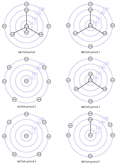
Figure 2.
The observed cointegration processes between the considered pairs, and its corresponding significance levels (1%, 5%, 10% and null) for the studied periods. The double-headed arrows represent the cointegration process between the commodity pairs.
Likewise, for the expected price transmission between the ethanol and corn in the American market, the Brazilian prices of ethanol and corn also show a cointegration for both tests. However, this behavior was not expected, since the Brazilian ethanol is primarily produced from sugarcane, while corn-based ethanol is in an initial state of production in the country. Agricultural production demands a considerable amount of energy, and this is reflected in the fuel consumption. The results suggest that ethanol prices and the markets of corn, cotton and Robusta coffee are linked, despite its production processes not being explicitly related.
3.1.2. Sub-Period 1 (January of 2011–May of 2012)
Table A2 and Figure 2b summarize the cointegration relation between the pairs of ethanol and each of the agricultural commodities during . It is possible to note that for the first sub-period, the cointegrations of ethanol with the sugar, cotton and Robusta coffee are still considered, and possibly influence the results in a macroscopic scale.
The Robusta coffee prices reached maximum values in the spot internal market, despite a good crop season during 2011/2012. Indeed, the Robusta coffee had an increase of 150% in export if compared with 2010. However, the same behavior was not observed for the Arabica coffee. From Table A1, Table A2, Table A3, Table A4, Table A5 and Table A6, we verify that for both coffees (Arabica and Robusta), the cointegration process with ethanol is only visible in the years of high production, since the coffee production alternates from a high to a low crop every year.
During , Brazil imported a significant volume of ethanol from the USA, due to a crop shortfall and an increase in the sugar international prices. This resulted in an increase in the prices for both commodities during the period.
In terms of the cotton commodity, one can note that its spot prices had the same pattern as those of the ethanol, with a higher peak at the beginning of the period, followed by an equilibrium during the middle of the TS and, finally, a bull market at the last year (see Figure 1).
3.1.3. Sub-Period 2 (May of 2012–November of 2013)
The cointegration test results during are summarized in Table A3 and Figure 2c. No cointegration process is observed for the tested pairs. One of the factors that help to describe this behavior is the currency exchange of the American dollar on this date. The prices of agricultural commodities usually have a negative correlation with the price of the dollar. Therefore, when the dollar gains force, the commodities become more expensive in other currencies, influencing negatively the demand. Alternatively, when the dollar becomes weaker, the commodities prices decrease in other currencies and then, as increasing demand occurs in the countries that import these commodities.
Brazil is an exporting country for the most part of these commodities. Thus, an increase in the R$ and US$ ratio increases the export, and the volume offered of the commodity in the internal market reduce, increasing their spot price.
3.1.4. Sub-Period 3 (November of 2013–September of 2015)
The sub-period is related to one difficult Brazilian socio–political cycle since it covers the presidential impeachment process. This process had important effects on several economy issues, namely in the energy sector. Figure 2d, shows the influence of corn and soybean commodities in the cattle market since the feed provided to the animals is mainly based on these products. Therefore, it is expected that the spot prices of the corn, soybean and live cattle may be cointegrated. From the Table A4 results, it is possible to note a cointegration between corn and ethanol. This effect can be transmitted to a cointegration process between the live cattle and the ethanol as well, since in the cattle production is not expected such a strong influence of an energy commodity as occurs for the cultivable commodities, namely the corn and soybean. The relation among the corn, live cattle and ethanol can be explained by its winter crop season production, since these products have a smaller volume of exports and, as a result, most of the production is directed for the internal market for animal consumption.
A cointegration between ethanol and soybean was not identified in any of the sub-periods. This can be explained by the relation between the spot and futures prices of the soybean in Brazil that are influenced by the international prices negotiated in the CME.
One can also observe a cointegration process involving the ETH-ARA pair during , that can be explained by the Arabica coffee production dynamics pointed out previously.
3.1.5. Sub-Period 4 (September of 2015–October of 2017)
The sub-period results for the cointegration test are listed in Table A5 and Figure 2e. For example, for , the demonstrates no cointegration processes among the pairs under analysis. On the other hand, this sub-period is related to political instability that affected directly the energy sector and may explain the no-cointegration relation among the pairs.
3.1.6. Sub-Period 5 (October of 2017–December of 2018)
The results obtained for point toward a price transmission in the ETH-ROB pair as it is shown in Table A6 and Figure 2f. Despite the dominance of the Arabica coffee production worldwide, the entrance of new countries offering Robusta coffee induced some price instability for the price of the two commodities. Additionaly, the same pattern of cointegration in the periods of large values for coffee commodities is observed for the ETH-ROB pair.
3.2. VECM Results
In this section, the VECM results are analyzed for the five sub-periods and the commodity pairs that revealed a cointegration process in the Johansen test (see Section 3.1), that is, , and . A plot scale adjustment to the FEVD model is applied to obtain a better visualization of the influence of the residuals of one variable in the forecast of the other.
3.2.1. Sub-Period 1
Here we cover the VECM results of the ETH-SUGAR, ETH-COT and ETH-ROB pairs.
Ethanol vs. Sugar
Equations (12) and (13) describe the ethanol price equation in the returns and the sugar price equation in the returns:
Table 2 shows the coefficients of the VECM adjusted for these equations. From the results in Table 2 we note that the adjustment coefficient () is statistically distinguishable from zero, which implies larger adjustments of the ethanol prices in disequilibrium, as we can confirm in Figure 3. Besides, the commodity tends to reach an equilibrium in steps. Therefore, the equation that allows the analysis of the long-run equilibrium relationship between the ETH-SUG prices can be formulated as:
Table 2.
The VECM for the ETH-SUG pair in . Significance levels: 10% (*), 5% (**), 1% (***) and 0.1% (****).
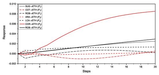
Figure 3.
The responses of the ethanol prices from an orthogonal impulse (OIR) in the agricultural commodities prices.
Then we applied the FEVD tool to measure the variance of the forecast error regarding the price shocks of the variables in the ethanol and sugar equations. It is possible to see small residuals from the ethanol prices in the sugar equation in Figure 5, with a decreasing influence along with the steps. The sugar commodity residuals are also present in the ethanol, but they increase along with the steps. It is reasonable to consider that similar to what was concluded in some studies [13,36,38,43] the sugar prices affect those of the ethanol in long-run for , but this co-movement relation is not observed in further periods considering structural breaks.
Ethanol vs. Cotton
Table 3 shows the VECM coefficients estimated for ETH-COT pair during , and one can note that the adjustment coefficient of the ethanol () is significantly different from zero. This means that the ethanol prices return back to equilibrium after a shock in the cotton prices within steps. The equation that describes the long-run relation between the variables can be written as:
Table 3.
The vector error correction models (VECM) for the ethanol (ETH)-cotton (COT) pair in . Significance levels: 10% (*), 5% (**), 1% (***) and 0.1% (****).
Figure 4 shows the stronger response of the cotton resulting from impulses (shocks) in the ethanol commodity when compared to the inverse case. This is confirmed by the parameter for the cotton equation, since it represents the autoregressive term of the ethanol on lag . Likewise, the FEVD in Figure 3 confirms a significant influence of ethanol residuals in the cotton prices forecast errors.
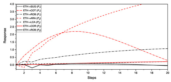
Figure 4.
The responses of the agricultural commodities prices from an orthogonal impulse (OIR) in the ethanol prices.
Ethanol vs. Robusta Coffee
The prices model of the ethanol and Robusta coffee are presented in Equations (17) and (18), respectively:
Table 4 presents the adjusted VECM for the ETH-ROB pair in . We can note that is also statistically different to zero for the ETH-ROB pair and the ethanol prices tend to return in equilibrium after steps. The term would indicate a short-run relation for the Robusta coffee (≈ 1 step). Nonetheless, the parameter is not significantly different from zero. Figure 3 and Figure 4 show that the impulse responses are different from those expected by the adjustment terms and , since the ethanol shows a short-run equilibrium to the shocks in the Robusta coffee prices. It also can be explained by the significant autoregressive terms and related to the Robusta coffee in the ethanol equation for the steps and , respectively. On the other hand, it was not possible to observe a short-run equilibrium in the Robusta coffee equation expected from the adjustment term. In fact, we merely verify that the Robusta coffee prices are influenced by shocks in the ethanol prices.
Table 4.
The VECM for the ETH-Robusta coffee (ROB) pair in . Significance levels: 10% (*), 5% (**), 1% (***) and 0.1% (****).
Figure 5 and Figure 6 depict the FEVD results validating this analysis, since we observe significant and increasing residuals in the forecast erros variance of the Robusta coffee. The following equation shows the long-run equilibrium between the pair:
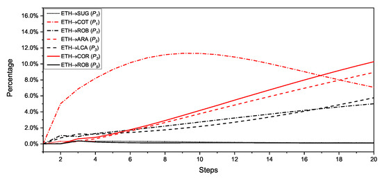
Figure 5.
The forecast error variance decomposition (FEVD) of the ethanol prices in the agricultural commodities prices.
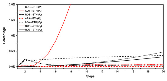
Figure 6.
The FEVD of the agricultural commodities prices in the ethanol prices.
3.2.2. Sub-Period 3
During the ETH-ARA, ETH-LCA and ETH-COR pairs resulting from the cointegration test are considered.
Ethanol vs. Arabica Coffee
Equations (20) and (21) present the VECM parameters adjusted for the ethanol and Arabica equations, respectively, as follows:
The VECM coefficients for the ethanol and Arabica coffee equations are listed in Table 5. The adjusted VECM reveal the high significance both for the adjustment coefficients and . Neverthless, is a positive large value, which is not usual for the VECM and can lead to a biased result, since may be interpreted as a strong significant influence of the ethanol prices (1st lag) in the Arabica coffee prices. Besides, in the Arabica coffee equation, is also a large value and its statistical significance could mean that the past values of the ethanol prices () result in significant weights in the Arabica coffee price at time t. The long-run relation between the prices is described by the Equation (22). Additionally, Figure 3, Figure 4, Figure 5 and Figure 6, representing the OIR and FEVD, demonstrate that shocks and residuals from the ethanol prices are transmitted to those of the Arabica coffee.
Table 5.
The VECM for the ETH-ARA pair in . Significance levels: 10% (*), 5% (**), 1% (***) and 0.1% (****).
Ethanol vs. Live Cattle
Equations (23) and (24) describe the ethanol and the live cattle price equations in the returns, respectively, as follows:
Table 6 shows the VECM adjusted parameters for the ETH-LCA pair equation. The VECM adjusted to the ETH-LCA pair shows an adjustment coefficient for live cattle commodity () statistically distinguishable from zero, instead of the significance that was common in the other pairs. Then, the live cattle prices tends to equilibrium after steps. The long-run equation is:
Table 6.
The VECM for the ETH-LCA pair in . Significance levels: 10% (*), 5% (**), 1% (***) and 0.1% (****).
On the contrary, the OIR and FEVD results evidenced from Figure 3, Figure 4, Figure 5 and Figure 6 point out a significant imbalance between the two prices. The OIR is similar to a step response (constant) for the ethanol resulting from an imbalance in live cattle price. On the other hand, we note a linear behavior for the live cattle after an impulse in the ethanol price. Differently from the dynamics observed for the US ethanol, cattle and field crops [41], the FEVD suggests a higher influence from the ethanol in the forecast error variances of the live cattle prices. By other words, in the Brazilian scenario, the ethanol prices are likely to describe live cattle prices forecasts than the opposite.
Ethanol vs. Corn
The adjusted VECM parameters are reported in Table 7. The cointegration of the ethanol and corn reflect the live cattle commodity. It is possible to note a mutual relation between the pair prices, so that the ethanol influences the corn prices and vice versa. Firstly, this is revealed by the significance of and and, therefore, we can assume that imbalances in the prices of the two commodities influence each one. The plots of the OIR in Figure 3 and Figure 4 suggest a similar imbalance pattern between the commodities. The intensity level of the corn prices imbalance is higher than the inverse situation. From the autoregressive terms of the prices equations, it is shown a significance for (ethanol term for lag ) and (corn term for lag ). This means that ethanol prices of one day in the past influence the corn prices in the present and the corn prices of three days in the past influence the ethanol prices in the present. The FEVD suggests mutual residual impact pattern in intensity level over the steps. Besides, this result differs from those observed in the US ethanol and corn relation (1994–2010) described in [40], concluding that the shocks in the US ethanol prices do not spill over those of the corn. The long-run relation between the pair follows the equation:
Table 7.
The VECM for the ETH-COR pair in . Significance levels: 10% (*), 5% (**), 1% (***) and 0.1% (****).
3.2.3. Sub-Period 5
The sub-period covers the ethanol vs. Robusta coffee VECM estimation, since it is the only pair that showed a cointegration process in the interval. It is worth highlighting that the ETH-ROB pair is the only one that showed cointegrated relation for differents sub-periods namely, and .
Ethanol vs. Robusta Coffee
The Equations (29) and (30) represent the ethanol and Robusta coffee equations, respectively, and Equation (31) denote the long-run equilibrium relation of the two TS as follows:
Table 8 lists the values of the VECM coefficients. Comparing these results with those obtained previously for the cointegration relation in for the same pair, we note that they reveal divergence in the price dynamics. Similarly to the ETH-LCA relation in and to the ETH-ROB previous results in Table 4, the ETH-ROB pair in demonstrates a non statistically significance for . Instead, we observe a significant , as well as statistically distinguishable from zero autoregressive terms related to ethanol prices in the past, in the Robusta coffee price equation ( and ). In addition, the OIR and FEVD applied to the pair suggest a lower imbalance for both commodities if compared to the adjusted model in . Besides, the FEVD shows a smaller influence of the residuals of the ethanol prices in the coffee prices, in terms of forecasting.
Table 8.
The VECM for the ETH-ROB pair in . Significance levels: 10% (*), 5% (**), 1% (***) and 0.1% (****).
4. Conclusions
This paper employed the bivariate analysis to investigate the ethanol prices transmission to the main Brazilian’s agricultural commodities by means of cointegration tests. The VECM estimation is evaluated whenever a cointegration process between the ethanol and a particular commodity is verified.
The results suggest a higher price transmission from the ethanol commodity to the agricultural commodities, than the opposite. The achieved results can be explained by the fact that agricultural commodities consume energy during their production stages. Therefore, important deviations or shocks in the prices of the ethanol can be transmitted significantly to the agricultural commodities. On the other hand, the ETH-SUG pair in the sub-period 1 and the ETH-COR pair in the sub-period 3 revealed mutual relations in their prices, where imbalances are mutually transmitted. Also, the soybean is the only agricultural commodity not showing cointegration with the ethanol in any of the sub-periods.
Author Contributions
These authors contributed equally to this work.
Funding
The authors wish to acknowledge the FAPESP (Sao Paulo Research Foundation), grants 2017/13815-3 and 2017/15517-0, for funding support.
Conflicts of Interest
The authors declare no conflict of interest.
Abbreviations
The following abbreviations are used in this manuscript:
| TS | Time series |
| VECM | Vector error correction model |
| VAR | Vector autoregression |
| OIR | Orthogonal impulse response |
| FEVD | Forecast error variance decomposition |
| CEPEA | Center for Advanced Studies on Applied Economics/University of Sao Paulo |
| GDP | Gross domestic product |
| FAO | Food and Agriculture Organization of the United Nations |
| CME | Chicago Mercantile Exchange |
| BMF/B3 | Brazilian Stock Exchange |
| ECM | Error correction model |
| ECT | Error correction term |
| ETH | Brazilian ethanol |
| SUG | Sugar |
| COT | Cotton |
| LCA | Live cattle |
| ARA | Arabica coffee |
| ROB | Robusta coffee |
| COR | Corn |
| SOY | Soybean |
| BP | Breakpoints |
| BIC | Bayesian information criterion |
| Sub-period 1 | |
| Sub-period 2 | |
| Sub-period 3 | |
| Sub-period 4 | |
| Sub-period 5 | |
| R$ | Brazilian reals |
| US$ | American dollar |
Appendix A
The following tables list the results of the Johansen cointegration test, orthogonal impulse response and forecast error variance decomposion.
Table A1.
The Johansen test for the full period. Significance levels: 10% (*), 5% (**) and 1% (***).
Table A1.
The Johansen test for the full period. Significance levels: 10% (*), 5% (**) and 1% (***).
| Pair | January of 2011–December of 2018 | ||
|---|---|---|---|
| Max-Eigen | Trace | ||
| ETH-SUG | 13.90 * | 17.67 | |
| 3.76 | 3.76 | ||
| ETH-COT | 21.1 *** | 26.6 *** | |
| 5.5 | 5.5 | ||
| ETH-LCA | 11.43 | 14.23 | |
| 2.81 | 2.81 | ||
| ETH-COR | 14.05 * | 18.05 * | |
| 4.0 | 4.0 | ||
| ETH-SOY | 10.63 | 15.43 | |
| 4.8 | 4.8 | ||
| ETH-ARA | 9.88 | 13.56 | |
| 3.67 | 3.67 | ||
| ETH-ROB | 14.30 * | 17.47 | |
| 3.17 | 3.17 | ||
Table A2.
The Johansen test for . Significance levels: 10% (*), 5% (**) and 1% (***).
Table A2.
The Johansen test for . Significance levels: 10% (*), 5% (**) and 1% (***).
| Pair | January of 2011–May of 2012 | ||
|---|---|---|---|
| Max-Eigen | Trace | ||
| ETH-SUG | 11.52 | 18.61 * | |
| 7.09 | 7.09 | ||
| ETH-COT | 14.87 * | 19.24 * | |
| 4.37 | 4.37 | ||
| ETH-LCA | 12.65 | 14.51 | |
| 1.86 | 1.86 | ||
| ETH-COR | 12.02 | 16.99 | |
| 4.97 | 4.97 | ||
| ETH-SOY | 11.57 | 13.08 | |
| 1.51 | 1.51 | ||
| ETH-ARA | 10.34 | 11.34 | |
| 1.00 | 1.00 | ||
| ETH-ROB | 15.18 * | 18.94 * | |
| 3.75 | 3.75 | ||
Table A3.
The Johansen test for .
Table A3.
The Johansen test for .
| Pair | May of 2012–November of 2013 | ||
|---|---|---|---|
| Max-Eigen | Trace | ||
| ETH-SUG | 6.80 | 10.37 | |
| 3.57 | 3.57 | ||
| ETH-COT | 5.57 | 7.95 | |
| 2.39 | 2.39 | ||
| ETH-LCA | 8.40 | 10.47 | |
| 2.08 | 2.08 | ||
| ETH-COR | 7.31 | 10.77 | |
| 3.46 | 3.46 | ||
| ETH-SOY | 7.54 | 11.38 | |
| 3.85 | 3.85 | ||
| ETH-ARA | 4.27 | 7.56 | |
| 3.29 | 3.29 | ||
| ETH-ROB | 3.81 | 5.25 | |
| 1.44 | 1.44 | ||
Table A4.
The Johansen test for . Significance levels: 10% (*), 5% (**) and 1% (***).
Table A4.
The Johansen test for . Significance levels: 10% (*), 5% (**) and 1% (***).
| Pair | November of 2013–September of 2015 | ||
|---|---|---|---|
| Max-Eigen | Trace | ||
| ETH-SUG | 13.34 | 15.51 | |
| 2.17 | 2.17 | ||
| ETH-COT | 8.63 | 9.35 | |
| 0.72 | 0.72 | ||
| ETH-LCA | 13.72 | 20.75 *** | |
| 7.03 | 7.03 | ||
| ETH-COR | 15.02 * | 17.92 * | |
| 2.89 | 2.89 | ||
| ETH-SOY | 8.70 | 9.57 | |
| 0.87 | 0.87 | ||
| ETH-ARA | 9.61 | 18.75 * | |
| 9.14 | 9.14 | ||
| ETH-ROB | 8.33 | 12.82 | |
| 4.49 | 4.49 | ||
Table A5.
The Johansen test for .
Table A5.
The Johansen test for .
| Pair | September of 2015–October of 2017 | ||
|---|---|---|---|
| Max-Eigen | Trace | ||
| ETH-SUG | 7.72 | 8.60 | |
| 0.88 | 0.88 | ||
| ETH-COT | 7.61 | 10.85 | |
| 3.23 | 3.23 | ||
| ETH-LCA | 5.58 | 6.64 | |
| 1.06 | 1.06 | ||
| ETH-COR | 4.88 | 6.51 | |
| 1.63 | 1.63 | ||
| ETH-SOY | 8.94 | 13.14 | |
| 4.20 | 4.20 | ||
| ETH-ARA | 11.66 | 14.55 | |
| 2.89 | 2.89 | ||
| ETH-ROB | 6.88 | 10.24 | |
| 3.35 | 3.35 | ||
Table A6.
The Johansen test for . Significance levels: 10% (*), 5% (**) and 1% (***).
Table A6.
The Johansen test for . Significance levels: 10% (*), 5% (**) and 1% (***).
| Pair | October of 2017–December of 2018 | ||
|---|---|---|---|
| Max-Eigen | Trace | ||
| ETH-SUG | 8.55 | 11.13 | |
| 2.58 | 2.58 | ||
| ETH-COT | 10.51 | 14.95 | |
| 4.43 | 4.43 | ||
| ETH-LCA | 7.33 | 10.39 | |
| 3.06 | 3.06 | ||
| ETH-COR | 11.03 | 14.45 | |
| 3.42 | 3.42 | ||
| ETH-SOY | 7.41 | 9.47 | |
| 2.06 | 2.06 | ||
| ETH-ARA | 9.87 | 14.56 | |
| 4.70 | 4.70 | ||
| ETH-ROB | 13.15 | 19.16 * | |
| 6.01 | 6.01 | ||
References
- Vedenov, D.; Wetzstein, M. Toward an optimal U.S. ethanol fuel subsidy. Energy Econ. 2008, 30, 2073–2090. [Google Scholar] [CrossRef]
- Bistafa, R.C. Impactos Econmicos da Nova Realidade da Exploração do Pré-Sal. Existe uma Ameaça ao Etanol? Master’s Thesis, Fundação Getulio Vargas—Escola de Economia de São Paulo, São Paulo, Brazil, 2016. [Google Scholar]
- Goldemberg, J. Ethanol for a sustainable energy future. Science 2007, 315, 808–810. [Google Scholar] [CrossRef] [PubMed]
- EPE. Análise de Conjuntura dos Biocombustíveis—Ano 2013; Technical Report; Empresa de Pesquisa Energética (EPE): Rio de Janeiro, Brazil, 2014. [Google Scholar]
- EPE. Análise de Conjuntura dos Biocombustíveis—Ano 2014; Technical Report; Empresa de Pesquisa Energética (EPE): Rio de Janeiro, Brazil, 2015. [Google Scholar]
- Oliveira, P.; Almeida, E. Determinants of fuel price control in Brazil and price policy options. In Proceedings of the 5th Latin American Energy Economics Meeting, Medellin, Colombia, 16–18 March 2015. [Google Scholar]
- Santos, G.R.; Garcia, E.A.; Shikida, P.F.A. A Crise na Produção do Etanol e as Interfaces com as Políticas Públicas. IPEA/DISET 2015, 39, 27–38. [Google Scholar]
- Quintino, D.; David, S.; Vian, C. Analysis of the relationship between ethanol spot and futures prices in Brazil. Int. J. Financ. Stud. 2017, 5, 11. [Google Scholar] [CrossRef]
- Mattos, F.L.; Franco da Silveira, R.L. The expansion of the Brazilian winter corn crop and its impact on price transmission. Int. J. Financ. Stud. 2018, 6, 45. [Google Scholar] [CrossRef]
- Farina, E.; Rodrigues, L. A Política Nacional de Biocombustíveis e os Ganhos de Eficincia no Setor Produtivo; Technical Report; FGV ENERGIA: Sao Paulo, Brazil, 2018. [Google Scholar]
- Janda, K.; Kristoufek, L. The Relationship between fuel and food prices: Methods, outcomes, and lessons for commodity price risk management. CAMA Work. Pap. 2019, 2019, 1–58. [Google Scholar] [CrossRef]
- David, S.A.; Machado, J.A.T.; Trevisan, L.R.; Inácio, C.M.C., Jr.; Lopes, A.M. Dynamics of commodities prices: Integer and fractional models. Fundam. Inform. 2017, 151, 389–408. [Google Scholar] [CrossRef]
- Serra, T.; Zilberman, D.; Gil, J. Price volatility in ethanol markets. Eur. Rev. Agric. Econ. 2010, 38, 259–280. [Google Scholar] [CrossRef]
- David, S.A.; Quintino, D.D.; Inacio, C.M.C., Jr.; Machado, J.A.T. Fractional dynamic behavior in ethanol prices series. J. Comput. Appl. Math. 2018, 339, 85–93. [Google Scholar] [CrossRef]
- Fowowe, B. Do oil prices drive agricultural commodity prices? Evidence from South Africa. Energy 2016, 104, 149–157. [Google Scholar] [CrossRef]
- Reboredo, J.C. Do food and oil prices co-move? Energy Policy 2012, 49, 456–467. [Google Scholar] [CrossRef]
- Nazlioglu, S.; Soytas, U. World oil prices and agricultural commodity prices: Evidence from an emerging market. Energy Econ. 2011, 33, 488–496. [Google Scholar] [CrossRef]
- Baffes, J. Oil spills on other commodities. Resour. Policy 2007, 32, 126–134. [Google Scholar] [CrossRef]
- Cha, K.S.; Bae, J.H. Dynamic impacts of high oil prices on the bioethanol and feedstock markets. Energy Policy 2011, 39, 753–760. [Google Scholar] [CrossRef]
- Chang, T.H.; Su, H.M. The substitutive effect of biofuels on fossil fuels in the lower and higher crude oil price periods. Energy 2010, 35, 2807–2813. [Google Scholar] [CrossRef]
- Chen, S.T.; Kuo, H.I.; Chen, C.C. Modeling the relationship between the oil price and global food prices. Appl. Energy 2010, 87, 2517–2525. [Google Scholar] [CrossRef]
- De Nicola, F.; Pace, P.D.; Hernandez, M.A. Co-movement of major energy, agricultural, and food commodity price returns: A time-series assessment. Energy Econ. 2016, 57, 28–41. [Google Scholar] [CrossRef]
- Koirala, K.H.; Mishra, A.K.; D’Antoni, J.M.; Mehlhorn, J.E. Energy prices and agricultural commodity prices: Testing correlation using copulas method. Energy 2015, 81, 430–436. [Google Scholar] [CrossRef]
- Obadi, S.; Korcek, M. Are food prices affected by crude oil price: Causality investigation. Rev. Integr. Bus. Econ. 2014, 3, 411–427. [Google Scholar]
- Ibrahim, M.H. Oil and food prices in Malaysia: A nonlinear ARDL analysis. Agric. Food Econ. 2015, 3, 2. [Google Scholar] [CrossRef]
- Pal, D.; Mitra, S.K. Diesel and soybean price relationship in the USA: Evidence from a quantile autoregressive distributed lag model. Empir. Econ. 2017, 52, 1609–1626. [Google Scholar] [CrossRef]
- Rafiq, S.; Bloch, H. Explaining commodity prices through asymmetric oil shocks: Evidence from nonlinear models. Resour. Policy 2016, 50, 34–48. [Google Scholar] [CrossRef]
- Zhang, C.; Qu, X. The effect of global oil price shocks on China’s agricultural commodities. Energy Econ. 2015, 51, 354–364. [Google Scholar] [CrossRef]
- Nazlioglu, S. World oil and agricultural commodity prices: Evidence from nonlinear causality. Energy Policy 2011, 39, 2935–2943. [Google Scholar] [CrossRef]
- Zafeiriou, E.; Arabatzis, G.; Karanikola, P.; Tampakis, S.; Tsiantikoudis, S. Agricultural commodities and crude oil prices: An empirical investigation of their relationship. Sustainability 2018, 10, 1199. [Google Scholar] [CrossRef]
- Ji, Q.; Bouri, E.; Roubaud, D.; Shahzad, S.J.H. Risk spillover between energy and agricultural commodity markets: A dependence-switching CoVaR-copula model. Energy Econ. 2018, 75, 14–27. [Google Scholar] [CrossRef]
- Hasanov, A.S.; Do, H.X.; Shaiban, M.S. Fossil fuel price uncertainty and feedstock edible oil prices: Evidence from MGARCH-M and VIRF analysis. Energy Econ. 2016, 57, 16–27. [Google Scholar] [CrossRef]
- Balcombe, K.; Bailey, A.; Brooks, J. Threshold effects in price transmission: The case of Brazilian wheat, maize, and soya prices. Am. J. Agric. Econ. 2007, 89, 308–323. [Google Scholar] [CrossRef]
- Baffes, J.; Gardner, B. The transmission of world commodity prices to domestic markets under policy reforms in developing countries. J. Policy Reform 2003, 6, 159–180. [Google Scholar] [CrossRef]
- Al-Maadid, A.; Caporale, G.M.; Spagnolo, F.; Spagnolo, N. Spillovers between food and energy prices and structural breaks. Int. Econ. 2017, 150, 1–18. [Google Scholar] [CrossRef]
- Bentivoglio, D.; Finco, A.; Bacchi, M. Interdependencies between biofuel, fuel and food prices: The case of the Brazilian ethanol market. Energies 2016, 9, 464. [Google Scholar] [CrossRef]
- Capitani, D.H.D.; Cruz, J.C., Jr.; Tonin, J.M. Integration and hedging efficiency between Brazilian and U.S. ethanol markets. Revista Contemporanea de Economia e Gestao 2018, 16, 93–117. [Google Scholar] [CrossRef]
- Dutta, A. Cointegration and nonlinear causality among ethanol-related prices: Evidence from Brazil. GCB Bioenerg. 2018, 10, 335–342. [Google Scholar] [CrossRef]
- Saghaian, S.H.; Nemati, M.; Walters, C.; Chen, B. Asymmetric price volatility transmission between U.S. biofuel, corn, and oil markets. J. Agric. Resour. Econ. 2018, 43, 46–60. [Google Scholar]
- Qiu, C.; Colson, G.; Escalante, C.; Wetzstein, M. Considering macroeconomic indicators in the food before fuel nexus. Energy Econ. 2012, 34, 2021–2028. [Google Scholar] [CrossRef]
- Bastianin, A.; Galeotti, M.; Manera, M. Causality and predictability in distribution: The ethanol–food price relation revisited. Energy Econ. 2014, 42, 152–160. [Google Scholar] [CrossRef]
- Bastianin, A.; Galeotti, M.; Manera, M. Ethanol and field crops: Is there a price connection? Food Policy 2016, 63, 53–61. [Google Scholar] [CrossRef]
- Kristoufek, L.; Janda, K.; Zilberman, D. Comovements of ethanol-related prices: Evidence from Brazil and the USA. GCB Bioenerg. 2016, 8, 346–356. [Google Scholar] [CrossRef]
- Serra, T.; Zilberman, D.; Gil, J.M.; Goodwin, B.K. Nonlinearities in the U.S. corn-ethanol-oil-gasoline price system. Agric. Econ. 2011, 42, 35–45. [Google Scholar] [CrossRef]
- Cabrera, B.L.; Schulz, F. Volatility linkages between energy and agricultural commodity prices. Energy Econ. 2016, 54, 190–203. [Google Scholar] [CrossRef]
- Bekiros, S.D.; Diks, C.G. The relationship between crude oil spot and futures prices: Cointegration, linear and nonlinear causality. Energy Econ. 2008, 30, 2673–2685. [Google Scholar] [CrossRef]
- He, L.; Xie, W. Who has the final say?: Market power versus price discovery in China’s sugar spot and futures markets. China Agric. Econ. Rev. 2012, 4, 379–390. [Google Scholar] [CrossRef]
- Ke, Y.; Li, C.; McKenzie, A.M.; Liu, P. Risk Transmission between Chinese and U.S. agricultural commodity futures markets—A CoVaR approach. Sustainability 2019, 11, 239. [Google Scholar] [CrossRef]
- Esposti, R.; Listorti, G. Agricultural price transmission across space and commodities during price bubbles. Agric. Econ. 2013, 44, 125–139. [Google Scholar] [CrossRef]
- Liu, Q.; An, Y. Information transmission in informationally linked markets: Evidence from US and Chinese commodity futures markets. J. Int. Money Finance 2011, 30, 778–795. [Google Scholar] [CrossRef]
- Campiche, J.L.; Bryant, H.L.; Richardson, J.W.; Outlaw, J.L. Examining the Evolving Correspondence Between Petroleum Prices and Agricultural Commodity Prices; Technical Report; Agricultural and Food Policy Center Department of Agricultural Economics: College Station, TX, USA, 2007. [Google Scholar]
- Ciaian, P.; d’Artis, K. Interdependencies in the energy–bioenergy–food price systems: A cointegration analysis. Resour. Energy Econ. 2011, 33, 326–348. [Google Scholar] [CrossRef]
- Ciaian, P.; d’Artis, K. Food, energy and environment: Is bioenergy the missing link? Food Policy 2011, 36, 571–580. [Google Scholar] [CrossRef]
- Natanelov, V.; Alam, M.J.; McKenzie, A.M.; Huylenbroeck, G.V. Is there co-movement of agricultural commodities futures prices and crude oil? Energy Policy 2011, 39, 4971–4984. [Google Scholar] [CrossRef]
- Nazlioglu, S.; Soytas, U. Oil price, agricultural commodity prices, and the dollar: A panel cointegration and causality analysis. Energy Econ. 2012, 34, 1098–1104. [Google Scholar] [CrossRef]
- Peri, M.; Baldi, L. Vegetable oil market and biofuel policy: An asymmetric cointegration approach. Energy Econ. 2010, 32, 687–693. [Google Scholar] [CrossRef]
- Peri, M.; Baldi, L. The effect of biofuel policies on feedstock market: Empirical evidence for rapeseed oil prices in EU. Resour. Energy Econ. 2013, 35, 18–37. [Google Scholar] [CrossRef]
- Rosa, F.; Vasciaveo, M. Volatility in US and Italian agricultural markets, interactions and policy evaluation. In Proceedings of the European Association of Agricultural Economists 123rd Seminar, Dublin, Ireland, 23–24 February 2012. [Google Scholar]
- Ziegelback, M.; Kastner, G. European rapeseed and fossil diesel: Threshold cointegration analysis and possible implications. In Proceedings of the 51st Annual Meeting of Gewisola, Corporative Agriculture: Between Market Needs and Social Expectations, Halle, Germany, 28–30 September 2011. [Google Scholar]
- Myers, R.J.; Johnson, S.R.; Helmar, M.; Baumes, H. Long-run and short-run co-movements in energy prices and the prices of agricultural feedstocks for biofuel. Am. J. Agric. Econ. 2014, 96, 991–1008. [Google Scholar] [CrossRef]
- Zhang, Z.; Lohr, L.; Escalante, C.; Wetzstein, M. Food versus fuel: What do prices tell us? Energy Policy 2010, 38, 445–451. [Google Scholar] [CrossRef]
- Mallory, M.L.; Hayes, D.J.; Irwin, S.A. How market efficiency and the theory of storage link corn and ethanol markets. Energy Econ. 2012, 34, 2157–2166. [Google Scholar] [CrossRef]
- Natanelov, V.; McKenzie, A.M.; Huylenbroeck, G.V. Crude oil–corn–ethanol–nexus: A contextual approach. Energy Policy 2013, 63, 504–513. [Google Scholar] [CrossRef]
- Saghaian, S.H. The impact of the oil sector on commodity prices: Correlation or causation? J. Agric. Appl. Econ. 2010, 42, 477–485. [Google Scholar] [CrossRef]
- Balcombe, K.; Rapsomanikis, G. Bayesian estimation and selection of nonlinear vector error correction models: The case of the sugar-ethanol-oil nexus in Brazil. Am. J. Agric. Econ. 2008, 90, 658–668. [Google Scholar] [CrossRef]
- Rajeaniova, M.; Pokriveak, J. The impact of biofuel policies on food prices in the European Union. J. Econ. (Ekonomicky Casopis) 2011, 59, 459–471. [Google Scholar]
- Wixson, S.E.; Katchova, A.L. Price asymmetric relationships in commodity and energy markets. In Proceedings of the 123rd EAAE Seminar Price Volatility and Farm Income Stabilisation, Modelling Outcomes and Assessing Market and Policy Based Responses, Dublin, Ireland, 23–24 February 2012. [Google Scholar]
- Pokriveak, J.; Rajeaniova, M. Crude oil price variability and its impact on ethanol prices. Agric. Econ. Czech 2011, 57, 394–403. [Google Scholar] [CrossRef]
- Bai, J.; Perron, P. Computation and analysis of multiple structural change models. J. Appl. Econ. 2003, 18, 1–22. [Google Scholar] [CrossRef]
- Zeileis, A.; Leisch, F.; Hornik, K.; Kleiber, C. Strucchange: An R Package for Testing for Structural Change in Linear Regression Models. J. Stat. Softw. 2002, 7, 1–38. [Google Scholar] [CrossRef]
- Zeileis, A.; Kleiber, C.; Krämer, W.; Hornik, K. Testing and dating of structural changes in practice. Comput. Stat. Data Anal. 2003, 44, 109–123. [Google Scholar] [CrossRef]
- Yao, Y.C. Estimating the number of change-points via Schwarz’ criterion. Stat. Probab. Lett. 1988, 6, 181–189. [Google Scholar] [CrossRef]
- Kingdom, F.A.; Prins, N. Chapter 9—Model comparisons. In Psychophysics, 2nd ed.; Kingdom, F.A., Prins, N., Eds.; Academic Press: San Diego, CA, USA, 2016; pp. 247–307. [Google Scholar]
- Da Costa, C.C.; Burnquist, H.L. Impactos do controle do preço da gasolina sobre o etanol biocombustível no Brasil. Estudos Econmicos (São Paulo) 2016, 46, 1003–1028. [Google Scholar] [CrossRef][Green Version]
- Granger, C.W.J. Some properties of time series data and their use in econometric model specification. J. Econ. 1981, 16, 121–130. [Google Scholar] [CrossRef]
- Engle, R.F.; Granger, C.W.J. Cointegration and error correction: Representation, estimation and testing. Econometrica 1987, 55, 251–276. [Google Scholar] [CrossRef]
- Murray, M.P. A Drunk and her dog: An illustration of cointegration and error correction. Am. Stat. 1994, 48, 37–39. [Google Scholar]
- Smith, A.; Harrison, R. A Drunk, Her Dog, and a Boyfriend: An Illustration of Multiple Cointegration and Error Correction; University of Canterbury, Department of Economics and Operations Research: Christchurch, New Zealand, 1994. [Google Scholar]
- Alexander, C. Correlation and Cointegration in Energy Markets. In Managing Energy Price Risk, Number 2; Risk Books: London, UK, 1999; pp. 291–304. [Google Scholar]
- Johansen, S. Statistical analysis of cointegration vectors. J. Econ. Dyn. Control 1988, 12, 231–254. [Google Scholar] [CrossRef]
- Johansen, S. Estimation and hypothesis testing of cointegration vectors in gaussian vector autoregressive models. Econometrica 1991, 59, 1551–1580. [Google Scholar] [CrossRef]
- Breitung, J.; Hassler, U. Inference on the cointegration rank in fractionally integrated processes. J. Econ. 2002, 110, 167–185. [Google Scholar] [CrossRef]
- Sargan, J.D. Wages and prices in the United Kingdom: A study in econometric methodology. Econom. Anal. Natl. Econ. Plan. 1964, 16, 25–54. [Google Scholar]
- Davidson, J.E.H.; Hendry, D.F.; Srba, F.; Yeo, S. Econometric modelling of the aggregate time-series relationship between consumers’ expenditure and income in the United Kingdom. Econ. J. 1978, 88, 661–692. [Google Scholar] [CrossRef]
- Cologni, A.; Manera, M. Oil prices, inflation and interest rates in a structural cointegrated VAR model for the G-7 countries. Energy Econ. 2008, 30, 856–888. [Google Scholar] [CrossRef]
- Juselius, K. The Cointegrated VAR Model: Methodology and Applications (Advanced Texts in Econometrics); Number 2; Oxford University Press: Oxford, UK, 2007; p. 477. [Google Scholar]
- Baillie, R.T.; Booth, G.G.; Tse, Y.; Zabotina, T. Price discovery and common factor models. J. Financ. Mark. 2002, 5, 309–321. [Google Scholar] [CrossRef]
- Mahadevan, R.; Asafu-Adjaye, J. Energy consumption, economic growth and prices: A reassessment using panel VECM for developed and developing countries. Energy Policy 2007, 35, 2481–2490. [Google Scholar] [CrossRef]


© 2019 by the authors. Licensee MDPI, Basel, Switzerland. This article is an open access article distributed under the terms and conditions of the Creative Commons Attribution (CC BY) license (http://creativecommons.org/licenses/by/4.0/).