Three-Step Projective Methods for Solving the Split Feasibility Problems

Abstract

In this paper, we focus on studying the split feasibility problem (SFP) in Hilbert spaces. Based on the CQ algorithm involving the self-adaptive technique, we introduce a three-step iteration process for approximating the solution of SFP. Then, the convergence results are established under mild conditions. Numerical experiments are provided to show the efficiency in signal processing. Some comparisons to various methods are also provided in this paper.

1. Introduction

In the present work, we aim to study the split feasibility problem (SFP), which is to find a point

$$x^{\ast }\in C\mathrm{such}\mathrm{that}A{x}^{\ast }\in Q,$$

(1)

where C and Q are non-empty, closed, and convex subsets of ${\mathbb{R}}^M$ and ${\mathbb{R}}^N$, and A is an $M\times N$ matrix. The SFP was first investigated in 1994 by Censor-Elfving [1]. Subsequently, Xu [2,3] also studied this problem in finite dimensional Hilbert spaces. There have also been real-world applications, such as image processing and signal recovery.

Censor et al. [4] (see also [5]) introduced the Split Inverse Problem (SIP). In this, let X and Y be two vector spaces and $A:X\to Y$ be a linear operator, such that two inverse problems are involved. Denote IP1 and IP2 by such inverse problems in X and Y, respectively. Given these data, the SIP is formulated as follows: find a point $x^{\ast }\in X$ that solves IP1, and such that the point $y^{\ast }=A{x}^{\ast }\in Y$ solves IP2.

It is known that the special case of the SFP can be reformulated to the following constrained minimization:

$${\displaystyle \underset{x\in C}{min}\parallel P_Q(Ax)-Ax\parallel .}$$

(2)

Due to this reformulation, it can be seen as the following linear equation:

$$x^{\ast }\in C\mathrm{and}A{x}^{\ast }=b.$$

(3)

In 2002, Byrne [6,7] introduced a new projection algorithm for the SFP. It was defined as follows:

$$x_{n+1}=P_C(x_n-{\tau }_n{A}^{\ast }(I-P_Q)A{x}_n)$$

(4)

where $P_C$ and $P_Q$ are projections onto C and Q, and $A^{\ast }$ denotes the adjoint operator of A. This method is often called the CQ algorithm. In this case, the convergence is guaranteed when the step-size ${\tau }_n$ is in $(0,\frac{2}{{\parallel A\parallel }^2})$, where ${\parallel A\parallel }^2$ is the spectral radius of the operator $A^{\ast }A$ and I stands for the identity operator. However, it should be noted that projections are not easy to be calculated, and also come with costs of computation.

In practical applications, the sets C and Q are usually defined by

$$C=\{x\in H_1:c(x)\le 0\}\mathrm{and}Q=\{y\in H_2:q(y)\le 0\},$$

(5)

where $c:H_1\to \mathbb{R}$ and $q:H_2\to \mathbb{R}$ are convex and sub-differential functions on $H_1$ and $H_2$. We always assume that $\partial c$ and $\partial q$ are bounded operators.

In 2004, Yang [8] presented the relaxed CQ algorithm, which follows from the idea of Fukushima [9]. The relaxed CQ algorithm, $P_C$ and $P_Q$, has been replaced by $P_{C_n}$ and $P_{Q_n}$, respectively, where $C_n$ and $Q_n$ are defined by

$$C_n=\{x\in H_1:c(x_n)\le \langle {\xi }_n,x_n-x\rangle \},$$

(6)

where ${\xi }_n\in \partial c(x_n)$ and

$$Q_n=\{y\in H_2:q(A{x}_n)\le \langle {\zeta }_n,A{x}_n-y\rangle \},$$

(7)

where ${\zeta }_n\in \partial q(A{x}_n)$. It is easily seen that $C_n\supset C$ and $Q_n\supset Q$ for all $n\ge 1$. Next, we set

$${\displaystyle f_n(x)=\frac{1}{2}{\parallel (I-P_{Q_n})Ax\parallel }^2,n\ge 1.}$$

(8)

In this case, we get

$$\nabla f_n(x)=A^{\ast }(I-P_{Q_n})Ax.$$

(9)

Since these sets are half-spaces, the computation for these projections is easy. However, if the step-size depends on the norm of operators, it is not an easy task to undertake. In fact, the relaxed CQ algorithm in a finite-dimentional Hilbert space was introduced by Yang [8] as follows:

$$x_{n+1}=P_{C_n}(x_n-{\tau }_n\nabla f_n(x_n)),$$

(10)

where ${\tau }_n{\in (0,2/\parallel A\parallel }^2)$. We note that the norm of A turned out to be costly in the computation. In particular, A is a dense matrix and has a large dimension.

To overcome this difficultly, in 2012, López et al. [10] presented a new step-size ${\tau }_n$ as follows:

$${\displaystyle {\tau }_n=\frac{{\rho }_n{f}_n(x_n)}{\parallel \nabla f_n(x_n){\parallel }^2},}$$

(11)

where $\{{\rho }_n\}$ is a sequence in $(0,4)$ such that ${\displaystyle \underset{n\in \mathbb{N}}{inf}{\rho }_n(4-{\rho }_n)>0}$. It was shown that $\{x_n\}$, with the step-size (11), converged weakly to a solution of SFP.

Another algorithm that can produce strong convergence is the Halpern-type algorithm. It is defined by

$$x_{n+1}={\alpha }_{n}u+(1-{\alpha }_n)P_{C_n}(x_n-{\tau }_n\nabla f_n(x_n)),$$

(12)

where $u\in H_1$ is fixed and ${\tau }_n$ is defined by (11). It was claimed that $\{x_n\}$ converges strongly to $P_{S}u$ when ${\alpha }_n\to 0$ and ${\displaystyle \sum _{n=1}^{\infty }{\alpha }_n=\infty .}$

Recently, in 2005, Qu-Xiu [11] suggested the relaxed CQ algorithm by using Armijo-linesearch in Euclidean spaces, and then Gibali et al. [12] generalized the results of Qu-Xiu [11] to real Hilbert spaces as follows:

$$\begin{array}{ccc}\hfill x_{n+1}& =& P_{C_n}(x_n-{\tau }_n\nabla f_n(y_n))\hfill \\ \hfill y_n& =& P_{C_n}(x_n-{\tau }_n\nabla f_n(x_n)),\hfill \end{array}$$

(13)

where $\sigma >0$, $\rho ,\mu \in (0,1)$, ${\tau }_n=\sigma {\rho }^{{\mu }_n}$, and ${\mu }_n$ is the smallest non-negative integer, such that

$${\tau }_n\parallel \nabla f_n(x_n)-\nabla f_n(y_n)\parallel \le \mu \parallel x_n-y_n\parallel .$$

(14)

It was shown that $\{x_n\}$ converges weakly to a solution of SFP. Various iterative methods have been established to solve the SFP and some related problems—see, for example, [2,3,4,5,13,14,15,16,17].

We aim to suggest a new three-step iteration process by using the CQ algorithm with step-sizes that employ the self-adaptive terminology. We remark that our assumptions do not depend on the operator norms, which is an easy task in practice. We then establish weak and strong convergence results under suitable conditions. Finally, we apply our results to compressed sensing. Some comparisons are also given to those of Yang [8], Gibali et al. [12], and López et al. [10].

Moreover, based on the three-step iterative methods, some convergence results, including its efficiency, have been established—see, for example, [18,19,20,21,22,23].

2. Basic Concepts

We next recall some useful basic concepts that will be used in our proof. Let H be a real Hilbert space. Let $T:H\to H$ be a nonlinear mapping. Then, T is called

(i)

nonexpansive if

$$\parallel Tx-Ty\parallel \le \parallel x-y\parallel ,forallx,y\in H.$$

(15)

(ii)

firmly nonexpansive if, for all $x,y\in H$,

$${\parallel Tx-Ty\parallel }^2\le \langle x-y,Tx-Ty\rangle .$$

(16)

A function $f:H\to \mathbb{R}$ is convex if

$$f(\lambda x+(1-\lambda )y)\le \lambda f(x)+(1-\lambda )f(y),forall\lambda \in (0,1),forallx,y\in H.$$

(17)

A function $f:H\to \mathbb{R}$ is weakly lower semi-continuous (w-lsc) at x if $x_n\rightharpoonup x$ implies

$${\displaystyle f(x)\le \underset{n\to \infty }{lim\; inf}f(x_n).}$$

(18)

The projection of a non-empty, closed, and convex set C onto H is defined by

$${\displaystyle P_{C}x:=arg\underset{y\in C}{min}{\parallel x-y\parallel }^2,x\in H.}$$

(19)

We note that $P_C$ and $I-P_C$ are firmly non-expansive. From [7], we know that if

$${\displaystyle f(x)=\frac{1}{2}{\parallel (I-P_Q)Ax\parallel }^2,}$$

then $\nabla f$ is ${\parallel A\parallel }^2$-Lipschitz continuous. Moreover, in real Hilbert spaces, we know that [24]

(i)

$\langle x-P_{C}x,z-P_{C}x\rangle \le 0$ for all $z\in C$;

(ii)

$\parallel P_{C}x-P_C{y\parallel }^2\le \langle P_{C}x-P_{C}y,x-y\rangle$ for all $x,y\in H$;

(iii)

$\parallel P_C{x-z\parallel }^2\le {\parallel x-z\parallel }^2-{\parallel P_{C}x-x\parallel }^2$ for all $z\in C$.

Lemma 1.

[25] Let H be a real Hilbert space and S be a non-empty, closed, and convex subset of H. Let $\{x_n\}$ be a sequence in H that satisfies the following conditions:

(i) 

For each $x\in S$, ${\displaystyle \underset{n\to \infty }{lim}\parallel x_n-x\parallel }$ exists;

(ii) 

${\omega }_w(x_n)\subset S$.

Then, $\{x_n\}$ converges weakly to a point in S.

Lemma 2.

[26] Let $\{s_n\}$ be a non-negative real sequence, such that

$$\begin{array}{ccc}\hfill s_{n+1}& \le & (1-{\alpha }_n)s_n+{\alpha }_n{\mu }_n,n\ge 1,\hfill \\ \hfill s_{n+1}& \le & s_n-{\lambda }_n+{\upsilon }_n,n\ge 1,\hfill \end{array}$$

(20)

where $\{{\alpha }_n\}\subseteq (0,1)$, $\{{\lambda }_n\}$ is a non-negative, real sequence, and $\{{\mu }_n\}$ and $\{{\upsilon }_n\}$ are real sequences such that

(i) 

${\displaystyle \sum _{n=1}^{\infty }{\alpha }_n=\infty }$;

(ii) 

${\displaystyle \underset{n\to \infty }{lim}{\upsilon }_n=0}$;

(iii) 

${lim}_{k\to \infty }{\lambda }_{n_k}=0$ implies ${\displaystyle \underset{k\to \infty }{lim\; sup}{\mu }_{n_k}\le 0}$ for any subsequence $\{n_k\}$ of $\{n\}$.

Then, ${\displaystyle \underset{n\to \infty }{lim}{s}_n=0}$.

Next, we propose Algorithms 1 and 2 for solving the split feasibility problem in Hilbert spaces.

3. Weak Convergence Result

We next introduce a new CQ algorithm and derive the weak convergence of the proposed method.

Algorithm 1: The proposed algorithm for weak convergence.

Choose $x_0\in H_1$. Let $x_{n+1}$ be iteratively generated by $$\begin{array}{ccc}\hfill z_n& =& x_n-{\tau }_n\nabla f_n(x_n)\hfill \\ \hfill y_n& =& z_n-{\gamma }_n\nabla f_n(z_n)\hfill \\ \hfill x_{n+1}& =& P_{C_n}(y_n-{\delta }_n\nabla f_n(y_n))\hfill \end{array}$$ (21) where $C_n$ is given as (6), $${\displaystyle {\tau }_n=\frac{{\rho }_n{f}_n(x_n)}{\parallel \nabla f_n(x_n){\parallel }^2},{\gamma }_n=\frac{{\rho }_n{f}_n(z_n)}{\parallel \nabla f_n(z_n){\parallel }^2}\mathrm{and}{\delta }_n=\frac{{\rho }_n{f}_n(y_n)}{\parallel \nabla f_n(y_n){\parallel }^2},0<{\rho }_n<4.}$$ (22)

Remark 1.

We see that Algorithm 1 is defined as the iterates $z_n$ and $y_n$ by a gradient method with the step-size ${\tau }_n$ and ${\gamma }_n$, respectively, and the iterate $x_{n+1}$ is defined by a relaxed CQ algorithm with the step-size ${\delta }_n$.

In this paper, we denote S by the solution set of SFP and assume that S is non-empty. Next, we prove its weak convergence theorem as follows:

Theorem 1.

Suppose ${\displaystyle \underset{n}{inf}{\rho }_n(4-{\rho }_n)>0}$. Then, $\{x_n\}$, defined by Algorithm 1, converges weakly to a point of S.

Proof. 

Let $\widehat{x}\in S$. Because $C\subseteq C_n$ and $Q\subseteq Q_n$, we have $\widehat{x}=P_C(\widehat{x})=P_{C_n}(\widehat{x})$ and $A\widehat{x}=P_Q(A\widehat{x})=P_{Q_n}(A\widehat{x})$. It follows that $\nabla f_n(\widehat{x})=0$. Then we obtain

$$\begin{array}{lll}\parallel x_{n+1}-\widehat{x}{\parallel }^2\hfill & =& \parallel P_{C_n}(y_n-{\delta }_n\nabla f_n(y_n))-\widehat{x}{\parallel }^2\hfill \\ & \le & \parallel y_n-{\delta }_n\nabla f_n(y_n)-\widehat{x}{\parallel }^2-{\parallel x_{n+1}-y_n+{\delta }_n\nabla f_n(y_n)\parallel }^2\hfill \\ & =& \parallel y_n-\widehat{x}{\parallel }^2+{\delta }_n^2{\parallel \nabla f_n(y_n)\parallel }^2-2{\delta }_n\langle y_n-\widehat{x},\nabla f_n(y_n)\rangle \hfill \\ & & -\parallel x_{n+1}-y_n+{\delta }_n\nabla f_n(y_n){\parallel }^2.\hfill \end{array}$$

(23)

From (23) and $\nabla f_n(\widehat{x})=0$, we see that

$$\begin{array}{ccc}\hfill \langle y_n-\widehat{x},\nabla f_n(y_n)\rangle & =& \langle y_n-\widehat{x},\nabla f_n(y_n)-\nabla f_n(\widehat{x})\rangle \hfill \\ & =& \langle y_n-\widehat{x},A^{\ast }(I-P_{Q_n})A{y}_n-A^{\ast }(I-P_{Q_n})A\widehat{x}\rangle \hfill \\ & =& \langle A{y}_n-A\widehat{x},(I-P_{Q_n})A{y}_n-(I-P_{Q_n})A\widehat{x}\rangle \hfill \\ & \ge & \parallel (I-P_{Q_n})A{y}_n{\parallel }^2\hfill \\ & =& 2f_n(y_n).\hfill \end{array}$$

(24)

We can also show that

$$\langle x_n-\widehat{x},\nabla f_n(x_n)\rangle \ge 2f_n(x_n)$$

(25)

and

$$\langle z_n-\widehat{x},\nabla f_n(z_n)\rangle \ge 2f_n(z_n).$$

(26)

So, by (26), it follows that

$$\begin{array}{ccc}\hfill \parallel y_n-\widehat{x}{\parallel }^2& =& \parallel z_n-{\gamma }_n\nabla f_n(z_n)-\widehat{x}{\parallel }^2\hfill \\ & =& \parallel z_n-\widehat{x}{\parallel }^2+{\gamma }_n^2{\parallel \nabla f_n(z_n)\parallel }^2-2{\gamma }_n\langle z_n-\widehat{x},\nabla f_n(z_n)\rangle \hfill \\ & \le & \parallel z_n-\widehat{x}{\parallel }^2+{\gamma }_n^2{\parallel \nabla f_n(z_n)\parallel }^2-4{\gamma }_n{f}_n(z_n).\hfill \end{array}$$

(27)

Moreover, by (25), we obtain

$$\begin{array}{ccc}\hfill \parallel z_n-\widehat{x}{\parallel }^2& =& \parallel x_n-{\tau }_n\nabla f_n(x_n)-\widehat{x}{\parallel }^2\hfill \\ & =& \parallel x_n-\widehat{x}{\parallel }^2+{\tau }_n^2{\parallel \nabla f_n(x_n)\parallel }^2-2{\tau }_n\langle x_n-\widehat{x},\nabla f_n(x_n)\rangle \hfill \\ & \le & \parallel x_n-\widehat{x}{\parallel }^2+{\tau }_n^2{\parallel \nabla f_n(x_n)\parallel }^2-4{\tau }_n{f}_n(x_n).\hfill \end{array}$$

(28)

Combining (23)–(28), we have

$$\begin{array}{lll}\parallel x_{n+1}-\widehat{x}{\parallel }^2& \le & \parallel x_n-\widehat{x}{\parallel }^2+{\tau }_n^2\parallel \nabla f_n(x_n){\parallel }^2-4{\tau }_n{f}_n(x_n)+{\gamma }_n^2{\parallel \nabla f_n(z_n)\parallel }^2\\ & & -4{\gamma }_n{f}_n(z_n)+{\delta }_n^2\parallel \nabla f_n(y_n){\parallel }^2-4{\delta }_n{f}_n(y_n)-{\parallel x_{n+1}-y_n+{\delta }_n\nabla f_n(y_n)\parallel }^2\\ & =& {\displaystyle \parallel x_n-\widehat{x}{\parallel }^2+\frac{{\rho }_n^2{f}_n^2(x_n)}{(\parallel \nabla f_n(x_n){{\parallel }^2)}^2}{\parallel \nabla f_n(x_n)\parallel }^2-\frac{4{\rho }_n{f}_n^2(x_n)}{\parallel \nabla f_n(x_n){\parallel }^2}}\\ & & +\frac{{\rho }_n^2{f}_n^2(z_n)}{(\parallel \nabla f_n(z_n){{\parallel }^2)}^2}\parallel \nabla f_n(z_n){\parallel }^2-\frac{4{\rho }_n{f}_n^2(z_n)}{\parallel \nabla f_n(z_n){\parallel }^2}+\frac{{\rho }_n^2{f}_n^2(y_n)}{(\parallel \nabla f_n(y_n){{\parallel }^2)}^2}{\parallel \nabla f_n(y_n)\parallel }^2\\ & & -\frac{4{\rho }_n{f}_n^2(y_n)}{\parallel \nabla f_n(y_n){\parallel }^2}-{\parallel x_{n+1}-y_n+{\delta }_n\nabla f_n(y_n)\parallel }^2\\ & =& {\displaystyle \parallel x_n-\widehat{x}{\parallel }^2+\frac{{\rho }_n^2{f}_n^2(x_n)}{\parallel \nabla f_n(x_n){\parallel }^2}-\frac{4{\rho }_n{f}_n^2(x_n)}{\parallel \nabla f_n(x_n){\parallel }^2}+\frac{{\rho }_n^2{f}_n^2(z_n)}{\parallel \nabla f_n(z_n){\parallel }^2}-\frac{4{\rho }_n{f}_n^2(z_n)}{\parallel \nabla f_n(z_n){\parallel }^2}}\\ & & +\frac{{\rho }_n^2{f}_n^2(y_n)}{\parallel \nabla f_n(y_n){\parallel }^2}-\frac{4{\rho }_n{f}_n^2(y_n)}{\parallel \nabla f_n(y_n){\parallel }^2}-{\parallel x_{n+1}-y_n+{\delta }_n\nabla f_n(y_n)\parallel }^2\\ & =& {\displaystyle \parallel x_n-\widehat{x}{\parallel }^2-{\rho }_n(4-{\rho }_n)\frac{f_n^2(x_n)}{\parallel \nabla f_n(x_n){\parallel }^2}-{\rho }_n(4-{\rho }_n)\frac{f_n^2(z_n)}{\parallel \nabla f_n(z_n){\parallel }^2}}\\ & & -{\rho }_n(4-{\rho }_n)\frac{f_n^2(y_n)}{\parallel \nabla f_n(y_n){\parallel }^2}-{\parallel x_{n+1}-y_n+{\delta }_n\nabla f_n(y_n)\parallel }^2.\end{array}$$

(29)

This implies that, since $0<{\rho }_n<4$,

$$\parallel x_{n+1}-\widehat{x}\parallel \le \parallel x_n-\widehat{x}\parallel .$$

(30)

Thus, ${\displaystyle \underset{n\to \infty }{lim}\parallel x_n-\widehat{x}\parallel }$ exists and $\{x_n\}$ is bounded. Since ${\displaystyle \underset{n\in \mathbb{N}}{inf}{\rho }_n(4-{\rho }_n)>0,}$ there is a $\rho$ such that ${\rho }_n(4-{\rho }_n)\ge \rho (4-\rho )>0.$ Again, from (29), it yields

$$\begin{array}{ccc}\hfill \parallel x_n-\widehat{x}{\parallel }^2-{\parallel x_{n+1}-\widehat{x}\parallel }^2& \ge & {\displaystyle \rho (4-\rho )\frac{f_n^2(x_n)}{\parallel \nabla f_n(x_n){\parallel }^2}+\rho (4-\rho )\frac{f_n^2(z_n)}{\parallel \nabla f_n(z_n){\parallel }^2}+\rho (4-\rho )\frac{f_n^2(y_n)}{\parallel \nabla f_n(y_n){\parallel }^2}}\hfill \\ & & +\parallel x_{n+1}-y_n+{\delta }_n\nabla f_n(y_n){\parallel }^2.\hfill \end{array}$$

(31)

So, we obtain

$$\begin{array}{ccc}\hfill {\displaystyle 0=\underset{n\to \infty }{lim}\parallel x_{n+1}-\widehat{x}{\parallel }^2-{\parallel x_n-\widehat{x}\parallel }^2}& \ge & {\displaystyle \underset{n\to \infty }{lim}[\rho (4-\rho )\frac{f_n^2(x_n)}{\parallel \nabla f_n(x_n){\parallel }^2}+\rho (4-\rho )\frac{f_n^2(z_n)}{\parallel \nabla f_n(z_n){\parallel }^2}}\hfill \\ & & +\rho (4-\rho )\frac{f_n^2(y_n)}{\parallel \nabla f_n(y_n){\parallel }^2}+\parallel x_{n+1}-y_n+{\delta }_n\nabla f_n(y_n){\parallel }^2]\hfill \\ & \ge & 0.\hfill \end{array}$$

(32)

This shows that

$$\begin{array}{c}\hfill {\displaystyle \underset{n\to \infty }{lim}\frac{f_n^2(x_n)}{\parallel \nabla f_n(x_n){\parallel }^2}=0,}\\ \hfill {\displaystyle \underset{n\to \infty }{lim}\frac{f_n^2(z_n)}{\parallel \nabla f_n(z_n){\parallel }^2}=0,}\\ \hfill {\displaystyle \underset{n\to \infty }{lim}\frac{f_n^2(y_n)}{\parallel \nabla f_n(y_n){\parallel }^2}=0,}\\ \hfill \underset{n\to \infty }{lim}{\parallel x_{n+1}-y_n+{\delta }_n\nabla f_n(y_n)\parallel }^2=0.\end{array}$$

(33)

We can check that $\{\parallel \nabla f_n(x_n)\parallel \}$ is bounded. So ${\displaystyle \underset{n\to \infty }{lim}{f}_n(x_n)=0}$. This means ${\displaystyle \underset{n\to \infty }{lim}\parallel (I-P_{Q_n})A{x}_n\parallel =0}$. Also ${\displaystyle \underset{n\to \infty }{lim}{f}_n(z_n)=\underset{n\to \infty }{lim}\parallel (I-P_{Q_n})A{z}_n\parallel =0}$ and ${\displaystyle \underset{n\to \infty }{lim}{f}_n(y_n)=\underset{n\to \infty }{lim}\parallel (I-P_{Q_n})A{y}_n\parallel =0}$.

Furthermore, from (33), we get

$${\displaystyle \underset{n\to \infty }{lim}\parallel x_{n+1}-y_n+{\delta }_n\nabla f_n(y_n)\parallel =0.}$$

(34)

We note that

$${\displaystyle {\delta }_n\parallel \nabla f_n(y_n)\parallel =\frac{{\rho }_n{f}_n(y_n)}{\parallel \nabla f_n(y_n){\parallel }^2}\parallel \nabla f_n(y_n)\parallel \to 0,\mathrm{as}n\to \infty .}$$

(35)

Hence, by (34) and (35), ${\displaystyle \underset{n\to \infty }{lim}\parallel x_{n+1}-y_n\parallel =0}$. Further, by (21) and ${\tau }_n\parallel \nabla f_n(x_n)\parallel \to 0$ as $n\to \infty$, we get ${\displaystyle \underset{n\to \infty }{lim}\parallel z_n-x_n\parallel =0}$. Since ${\gamma }_n\parallel \nabla f_n(x_n)\parallel \to 0$ as $n\to \infty$, we also get ${\displaystyle \underset{n\to \infty }{lim}\parallel y_n-z_n\parallel =0.}$ Hence ${\displaystyle \underset{n\to \infty }{lim}\parallel x_{n+1}-x_n\parallel =0}$.

By the boundedness of $\{x_n\}$, the set ${\omega }_w(x_n)$ is non-empty. Let $x^{\ast }\in {\omega }_w(x_n)$. Then, there is a subsequence $\{x_{n_k}\}$ of $\{x_n\}$ that $x_{n_k}\rightharpoonup x^{\ast }\in H_1$.

Next, we show that $x^{\ast }$ is in S. Since $x_{n_k+1}\in C_{n_k}$, by the definition of $C_{n_k}$, we get

$$c(x_{n_k})\le \langle {\xi }_{n_k},x_{n_k}-x_{n_k+1}\rangle$$

(36)

where ${\xi }_{n_k}\in \partial c(x_{n_k})$. It follows, by the boundedness of $\partial c$, that

$$\begin{array}{ccc}\hfill c(x_{n_k})& \le & \parallel {\xi }_{n_k}\parallel \parallel x_{n_k}-x_{n_k+1}\parallel \hfill \\ & \to & 0,\mathrm{as}k\to \infty .\hfill \end{array}$$

(37)

By the w-lsc of c, $x_{n_k}\rightharpoonup x^{\ast }$ and (37), we see that

$${\displaystyle c(x^{\ast })\le \underset{k\to \infty }{lim\; inf}c(x_{n_k})\le 0.}$$

(38)

Thus, $x^{\ast }\in C$.

Next, we will show that $A{x}^{\ast }\in Q$. Since $P_{Q_{n_k}}(A{x}_{n_k})\in Q_{n_k}$,

$$q(A{x}_{n_k})\le \langle {\eta }_{n_k},A{x}_{n_k}-P_{Q_{n_k}}(A{x}_{n_k})\rangle$$

(39)

where ${\eta }_{n_k}\in \partial q(A{x}_{n_k})$. So, we obtain

$$\begin{array}{ccc}\hfill q(A{x}_{n_k})& \le & \parallel {\eta }_{n_k}\parallel \parallel A{x}_{n_k}-P_{Q_{n_k}}(A{x}_{n_k})\parallel \hfill \\ & \to & 0,\mathrm{as}k\to \infty .\hfill \end{array}$$

(40)

The w-lsc of q and (40) give that

$${\displaystyle q(A{x}^{\ast })\le \underset{k\to \infty }{lim\; inf}q(A{x}_{n_k})\le 0.}$$

(41)

Thus, $A{x}^{\ast }\in Q$. By Lemma 1, we can deduce that $\{x_n\}$ converges weakly to a point in S. □

4. Strong Convergence Result

We next discuss the strong convergence of the sequence generated by the Halpern-type iteration.

Algorithm 2: The proposed algorithm for strong convergence.

Choose $x_0\in H_1$. Assume $x_n$, $z_n$ and $y_n$ have been constructed. Compute the sequence $x_{n+1}$ by $$\begin{array}{ccc}\hfill z_n& =& x_n-{\tau }_n\nabla f_n(x_n)\hfill \\ \hfill y_n& =& z_n-{\gamma }_n\nabla f_n(z_n)\hfill \\ \hfill x_{n+1}& =& {\alpha }_{n}u+(1-{\alpha }_n)P_{C_n}(y_n-{\delta }_n\nabla f_n(y_n))\hfill \end{array}$$ (42) where $u\in H_1$ and $\{{\alpha }_n\}\subset (0,1)$, $C_n$ is given as (6), $${\displaystyle {\tau }_n=\frac{{\rho }_n{f}_n(x_n)}{\parallel \nabla f_n(x_n){\parallel }^2},{\gamma }_n=\frac{{\rho }_n{f}_n(z_n)}{\parallel \nabla f_n(z_n){\parallel }^2}\mathrm{and}{\delta }_n=\frac{{\rho }_n{f}_n(y_n)}{\parallel \nabla f_n(y_n){\parallel }^2},0<{\rho }_n<4.}$$ (43)

Theorem 2.

Assume that $\{{\alpha }_n\}$ and $\{{\rho }_n\}$ satisfy the conditions:

(a) 

${\displaystyle \underset{n\to \infty }{lim}{\alpha }_n=0}$ and ${\displaystyle \sum _{n=1}^{\infty }{\alpha }_n=\infty }$;

(b) 

${\displaystyle \underset{n}{inf}{\rho }_n(4-{\rho }_n)>0.}$

Then, $\{x_n\}$, defined by Algorithm 2, converges strongly to $P_{S}u$.

Proof. 

Set $\widehat{x}=P_{S}u$. By using the same argument as in Theorem 1, we can show that

$$\begin{array}{ccc}\hfill \parallel P_{C_n}(y_n-{\delta }_n\nabla f_n(y_n))-\widehat{x}{\parallel }^2& \le & {\displaystyle \parallel y_n-\widehat{x}{\parallel }^2-{\rho }_n(4-{\rho }_n)\frac{f_n^2(y_n)}{\parallel \nabla f_n(y_n)\parallel }}\hfill \\ & & -\parallel P_{C_n}(y_n-{\delta }_n\nabla f_n(y_n))-y_n+{\delta }_n\nabla f_n(y_n){\parallel }^2.\hfill \end{array}$$

(44)

So,

$$\begin{array}{c}\hfill {\displaystyle \parallel y_n-\widehat{x}{\parallel }^2\le {\parallel z_n-\widehat{x}\parallel }^2-{\rho }_n(4-{\rho }_n)\frac{f_n^2(z_n)}{\parallel \nabla f_n(z_n){\parallel }^2}}\end{array}$$

(45)

and

$${\displaystyle \parallel z_n-\widehat{x}{\parallel }^2\le {\parallel x_n-\widehat{x}\parallel }^2-{\rho }_n(4-{\rho }_n)\frac{f_n^2(x_n)}{\parallel \nabla f_n(x_n){\parallel }^2}.}$$

(46)

Also, we obtain

$$\begin{array}{ccc}\hfill \parallel x_{n+1}-\widehat{x}{\parallel }^2& =& \parallel {\alpha }_n(u-\widehat{x})+(1-{\alpha }_n)(P_{C_n}(y_n-{\delta }_n\nabla f_n(y_n))-\widehat{x}){\parallel }^2\hfill \\ & \le & (1-{\alpha }_n){\parallel P_{C_n}(y_n-{\delta }_n\nabla f_n(y_n))-\widehat{x}\parallel }^2+2{\alpha }_n\langle u-\widehat{x},x_{n+1}-\widehat{x}\rangle .\hfill \end{array}$$

(47)

Combining (44)–(47), we obtain

$$\begin{array}{ccc}\hfill \parallel x_{n+1}-\widehat{x}{\parallel }^2& \le & {\displaystyle (1-{\alpha }_n){\parallel x_n-\widehat{x}\parallel }^2-(1-{\alpha }_n){\rho }_n(4-{\rho }_n)\frac{f_n^2(x_n)}{\parallel \nabla f_n(x_n){\parallel }^2}}\hfill \\ & & {\displaystyle -(1-{\alpha }_n){\rho }_n(4-{\rho }_n)\frac{f_n^2(z_n)}{\parallel \nabla f_n(z_n){\parallel }^2}-(1-{\alpha }_n){\rho }_n(4-{\rho }_n)\frac{f_n^2(y_n)}{\parallel \nabla f_n(y_n){\parallel }^2}}\hfill \\ & & -(1-{\alpha }_n){\parallel P_{C_n}(y_n-{\delta }_n\nabla f_n(y_n))-y_n+{\delta }_n\nabla f_n(y_n)\parallel }^2\hfill \\ & & +2{\alpha }_n\langle u-\widehat{x},x_{n+1}-\widehat{x}\rangle .\hfill \end{array}$$

(48)

Next, we will show that $\{x_n\}$ is bounded. Again, using (44)–(46), we get

$$\begin{array}{ccc}\hfill \parallel x_{n+1}-\widehat{x}\parallel & =& \parallel {\alpha }_{n}u+(1-{\alpha }_n)P_{C_n}(y_n-{\delta }_n\nabla f_n(y_n))-\widehat{x}\parallel \hfill \\ & \le & {\alpha }_n\parallel u-\widehat{x}\parallel +(1-{\alpha }_n)\parallel y_n-\widehat{x}\parallel \hfill \\ & \le & {\alpha }_n\parallel u-\widehat{x}\parallel +(1-{\alpha }_n)\parallel z_n-\widehat{x}\parallel \hfill \\ & \le & {\alpha }_n\parallel u-\widehat{x}\parallel +(1-{\alpha }_n)\parallel x_n-\widehat{x}\parallel .\hfill \end{array}$$

(49)

This shows that $\{x_n\}$ is bounded. From Lemma 2 and (48), we set

$$\begin{array}{ccc}\hfill s_n& =& \parallel x_n-\widehat{x}{\parallel }^2;\hfill \\ \hfill {\upsilon }_n& =& 2{\alpha }_n\langle u-\widehat{x},x_{n+1}-\widehat{x}\rangle ;\hfill \\ \hfill {\mu }_n& =& 2\langle u-\widehat{x},x_{n+1}-\widehat{x}\rangle ;\hfill \\ \hfill {\lambda }_n& =& {\displaystyle (1-{\alpha }_n){\parallel P_{C_n}(y_n-{\delta }_n\nabla f_n(y_n))-y_n+{\delta }_n\nabla f_n(y_n)\parallel }^2+(1-{\alpha }_n){\rho }_n(4-{\rho }_n)\frac{f_n^2(x_n)}{\parallel \nabla f_n(x_n){\parallel }^2}}\hfill \\ & & {\displaystyle +(1-{\alpha }_n){\rho }_n(4-{\rho }_n)\frac{f_n^2(y_n)}{\parallel \nabla f_n(y_n){\parallel }^2}+(1-{\alpha }_n){\rho }_n(4-{\rho }_n)\frac{f_n^2(z_n)}{\parallel \nabla f_n(z_n){\parallel }^2}.}\hfill \end{array}$$

(50)

So (48) can be transformed to the inequalities

$$\begin{array}{ccc}\hfill s_{n+1}& \le & (1-{\alpha }_n)s_n+{\alpha }_n{\mu }_n,n\ge 1\hfill \\ \hfill s_{n+1}& \le & s_n-{\lambda }_n+{\upsilon }_n.\hfill \end{array}$$

(51)

Let $\{n_k\}$ be a subsequence of $\{n\}$, such that

$${\displaystyle \underset{k\to \infty }{lim}{\lambda }_{n_k}=0.}$$

(52)

Then, we have

$$\begin{array}{ll}{\displaystyle \underset{k\to \infty }{lim}}& (1-{\alpha }_{n_k}){\parallel P_{C_{n_k}}(y_{n_k}-{\delta }_{n_k}\nabla f_{n_k}(y_{n_k}))-y_{n_k}+{\delta }_{n_k}\nabla f_{n_k}(y_{n_k})\parallel }^2\\ & {\displaystyle +(1-{\alpha }_{n_k}){\rho }_{n_k}(4-{\rho }_{n_k})\frac{f_{n_k}^2(x_{n_k})}{\parallel \nabla f_{n_k}(x_{n_k}){\parallel }^2}+(1-{\alpha }_{n_k}){\rho }_{n_k}(4-{\rho }_{n_k})\frac{f_{n_k}^2(z_{n_k})}{\parallel \nabla f_{n_k}(z_{n_k}){\parallel }^2}}\\ & {\displaystyle +(1-{\alpha }_{n_k}){\rho }_{n_k}(4-{\rho }_{n_k})\frac{f_{n_k}^2(y_{n_k})}{\parallel \nabla f_{n_k}(y_{n_k}){\parallel }^2}=0}\end{array}$$

(53)

which implies by our assumptions that

$${\displaystyle \begin{array}{c}\frac{f_{n_k}^2(x_{n_k})}{\parallel \nabla f_{n_k}(x_{n_k}){\parallel }^2}\to 0,\frac{f_{n_k}^2(z_{n_k})}{\parallel \nabla f_{n_k}(z_{n_k}){\parallel }^2}\to 0,\frac{f_{n_k}^2(y_{n_k})}{\parallel \nabla f_{n_k}(y_{n_k}){\parallel }^2}\to 0\mathrm{and}\\ \parallel P_{C_{n_k}}(y_{n_k}-{\delta }_{n_k}\nabla f_{n_k}(y_{n_k}))-y_{n_k}+{\delta }_{n_k}\nabla f_{n_k}(y_{n_k})\parallel \to 0\end{array}}$$

as $k\to \infty$. Since $\{\parallel \nabla f_{n_k}(x_{n_k})\parallel \}$, $\{\parallel \nabla f_{n_k}(z_{n_k})\parallel \}$ and $\{\parallel \nabla f_{n_k}(y_{n_k})\parallel \}$ are bounded, it follows that $f_{n_k}(x_{n_k})\to 0$, $f_{n_k}(z_{n_k})\to 0$ and $f_{n_k}(y_{n_k})\to 0$ as $k\to \infty$. We also get ${\displaystyle \underset{k\to \infty }{lim}\parallel (I-P_{Q_{n_k}})A{x}_{n_k}\parallel =0}$, ${\displaystyle \underset{k\to \infty }{lim}\parallel (I-P_{Q_{n_k}})A{z}_{n_k}\parallel =0}$ and ${\displaystyle \underset{k\to \infty }{lim}\parallel (I-P_{Q_{n_k}})A{y}_{n_k}\parallel =0}$.

As in Theorem 1, we can show that ${\omega }_w(x_{n_k})\subset S$. Hence, there is a subsequence $\{x_{n_{k_i}}\}$ of $\{x_{n_k}\}$, such that $x_{n_{k_i}}\rightharpoonup x^{\ast }\in S$. So, we obtain

$$\begin{array}{ccc}\hfill {\displaystyle \underset{k\to \infty }{lim\; sup}\langle u-\widehat{x},x_{n_k}-\widehat{x}\rangle }& =& {\displaystyle \underset{i\to \infty }{lim}\langle u-\widehat{x},x_{n_{k_i}}-\widehat{x}\rangle }\hfill \\ & =& \langle u-\widehat{x},x^{\ast }-\widehat{x}\rangle \hfill \\ & \le & 0.\hfill \end{array}$$

(54)

On the other hand, we see that

$$\begin{array}{ccc}\hfill \parallel x_{n_k+1}-y_{n_k}\parallel & =& \parallel {\alpha }_{n_k}u+(1-{\alpha }_{n_k})P_{C_{n_k}}(y_{n_k}-{\delta }_{n_k}\nabla f_{n_k}(y_{n_k}))-y_{n_k}\parallel \hfill \\ & \le & {\alpha }_{n_k}\parallel u-y_{n_k}\parallel +(1-{\alpha }_{n_k})\parallel P_{C_{n_k}}(y_{n_k}-{\delta }_{n_k}\nabla f_{n_k}(y_{n_k}))-y_{n_k}\parallel \hfill \\ & \le & {\alpha }_{n_k}\parallel u-y_{n_k}\parallel +(1-{\alpha }_{n_k})\parallel P_{C_{n_k}}(y_{n_k}-{\delta }_{n_k}\nabla f_{n_k}(y_{n_k}))-y_{n_k}+{\delta }_{n_k}\nabla f_{n_k}(y_{n_k})\parallel \hfill \\ & & +(1-{\alpha }_{n_k}){\delta }_{n_k}\parallel \nabla f_{n_k}(y_{n_k})\parallel \hfill \\ & \to & 0\mathrm{as}k\to \infty .\hfill \end{array}$$

(55)

We see that

$${\displaystyle \underset{k\to \infty }{lim}\parallel z_{n_k}-x_{n_k}\parallel =0\mathrm{and}\underset{k\to \infty }{lim}\parallel y_{n_k}-z_{n_k}\parallel =0.}$$

Hence, we obtain

$$\begin{array}{ccc}\hfill \parallel x_{n_k+1}-x_{n_k}\parallel & \le & \parallel x_{n_k+1}-y_{n_k}\parallel +\parallel y_{n_k}-z_{n_k}\parallel +\parallel z_{n_k}-x_{n_k}\parallel \hfill \\ & \to & 0\mathrm{as}k\to \infty .\hfill \end{array}$$

(56)

By (54) and (56), we obtain

$${\displaystyle \underset{k\to \infty }{lim\; sup}\langle u-\widehat{x},x_{n_k+1}-\widehat{x}\rangle \le 0.}$$

(57)

Hence, we get

$${\displaystyle \underset{k\to \infty }{lim\; sup}{\mu }_{n_k}\le 0.}$$

(58)

By Lemma 2, we can deduce that $\{x_n\}$ converges strongly to $\widehat{x}=P_{S}u$. □

5. Numerical Examples

Finally, we provide numerical experiments of the compressed sensing in signal recovery. We demonstrate the performance of the relaxed CQ algorithms defined by Yang [8], López et al. [10], Gibali et al. [12] and our CQ algorithms. The compressed sensing can be modeled as the linear equation:

$$y=Ax+\epsilon ,$$

(59)

where $x\in {\mathbb{R}}^N$ is a recovered vector with m non-zero components, $y\in {\mathbb{R}}^M$ is the observed data with noisy $\epsilon$, and $A:{\mathbb{R}}^N\to {\mathbb{R}}^M$$(M<N)$. It is noted that (59) can be seen as solving the LASSO problem:

$${\displaystyle \underset{x\in {\mathbb{R}}^N}{min}\frac{1}{2}{\parallel y-Ax\parallel }^2\mathrm{subject}\mathrm{to}{\parallel x\parallel }_1\le t,}$$

(60)

where $t>0$. In particular, in case $C=\{x\in {\mathbb{R}}^N:\parallel x{\parallel }_1\le t\}$ and $Q=\{y\}$, the LASSO problem can be considered as the SFP (1). From this point of view, we can apply the CQ algorithm to solve (60).

In our experiment, one matrix $A\in {\mathbb{R}}^{M\times N}$ is generated from a normal distribution with mean zero and invariance one. The sparse vector $x\in {\mathbb{R}}^N$ is generated from uniform distribution in the interval $[-1,1]$ with m nonzero elements. The observation y is generated by white Gaussian noise with signal-to-noise ratio SNR=40. Let $t=m$ and $x_1=0$.

The stopping criterion is defined by the mean square error (MSE):

$${\displaystyle \mathrm{MSE}=\frac{1}{N}{\parallel \widehat{x}-x\parallel }_2^2<{10}^{-5},}$$

(61)

where $\widehat{x}$ is an approximated signal of x.

In what follows, let ${\displaystyle {\tau }_n=\frac{1}{{\parallel A\parallel }^2}}$ in the CQ algorithm (10) by Yang [8], ${\displaystyle {\tau }_n=\frac{{\rho }_n{\parallel Ax-y\parallel }^2}{2\parallel A^T{(Ax-y)\parallel }^2}}$ with ${\rho }_n=2$ in (11) of López et al. [10], ${\tau }_n$ defined by (14) with $\sigma =1$, $\rho =\mu =0.5$ in that of Gibali et al. [12] and ${\tau }_n,{\gamma }_n$,${\delta }_n$ defined by (22) with ${\rho }_n=2$. The numerical results are reported as follows.

From

Table 1. Number of iterations for Algorithm 1.

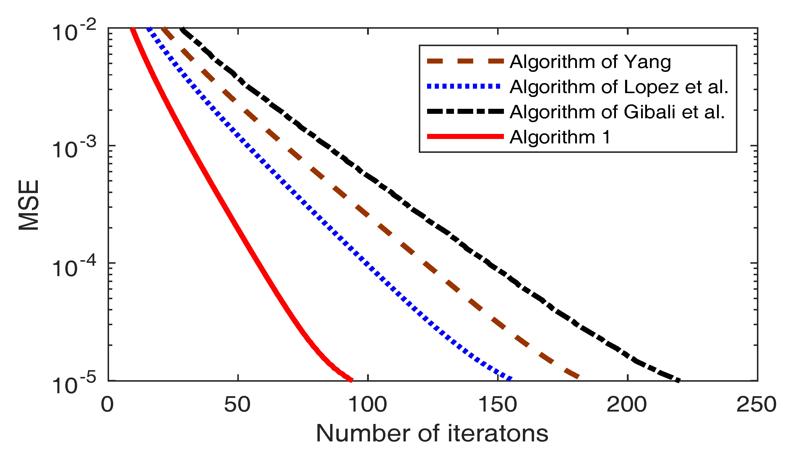
Case 1: $\mathit{N}=512$, $\mathit{M}=256$	Yang (10)	López et al. (11)	Gibali et al. (13)	Algorithm 1
$m=10$	74	65	106	39
$m=20$	217	184	246	111
Case 2: $N=4096$, $M=2048$	Yang (10)	López et al. (11)	Gibali et al. (13)	Algorithm 1
$m=100$	87	77	117	48
$m=200$	184	156	220	94

and Figure 1 and Figure 2, we observe that the convergence behavior of Algorithm 1 outperforms those of Yang [8], López et al. [10], Gibali et al. [12]. Indeed, Algorithm 1 has less number of iterations than other methods.

Next, we discuss the strong convergence of the relaxed CQ algorithm (12) by López et al. [10] and Algorithm 2. We set each step-sizes ${\tau }_n$ as in the weak convergence and let ${\displaystyle {\alpha }_n=\frac{1}{100n+1}}$. The initial vector $x_1=0$ and u is generated randomly. Then, we have the following numerical results.

From

Table 2. Number of iterations for Algorithm 2.

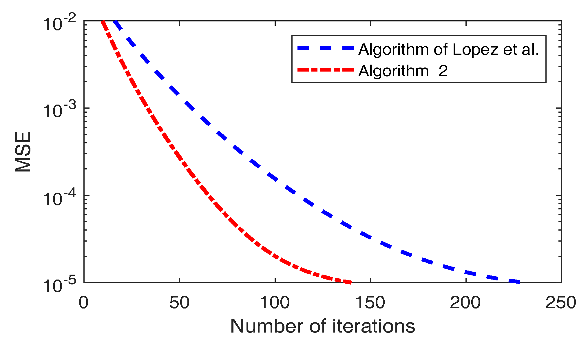
Case 1: $\mathit{N}=512$, $\mathit{M}=256$	López et al. (12)	Algorithm 2
$m=10$	85	43
$m=20$	119	64
Case 2: $N=4096$, $M=2048$	López et al. (12)	Algorithm 2
$m=100$	85	48
$m=200$	230	140

and Figure 3 and Figure 4, it is observed that Algorithm 2 has a smaller number of iterations than that of López et al. [10].

We provide the numerical examples in $L_2$-space, which is an infinite Hilbert space, by using Algorithm 2. Let $H_1=H_2=L_2[0,1]$ with the inner product given by

$$\langle f,g\rangle ={\int }_0^{1}f(t)g(t)dt.$$

Let $C=\{x\in L_2[0,1]:\parallel x{\parallel }_{L_2}\le 1\}$ and $Q=\{x\in L_2[0,1]:\langle x,\frac{t}{2}\rangle \le 0\}$. Find $x\in C$ such that $Ax\in Q$, where $(Ax)(t)=\frac{x(t)}{2}$. We take ${\alpha }_n={\displaystyle \frac{1}{10n+1}}$, ${\rho }_n=1.75$. The stopping criterion is defined by

$$E_n={\displaystyle \frac{1}{2}}{\parallel A{x}_n-P_{Q}A{x}_n\parallel }_{L_2}^2<{10}^{-4}.$$

From

Table 3. Numberof iterations for Algorithm 2 in $L_2$-space.

		López et al. (12)	Algorithm 2
$u=t$	No. of Iter.	9	4
$x_1=7t^2+2$	cpu (time)	6.3707	4.0171
$u=t+1$	No. of Iter.	9	4
$x_1=4t^2+t+3$	cpu (time)	6.5169	4.1789
$u=t^2$	No. of Iter.	10	4
$x_1=2t^2+3e^t$	cpu (time)	9.4818	5.5274
$u=t^3$	No. of Iter.	6	3
$x_1=5t^3+sin(t)+1$	cpu (time)	3.7478	2.9404

and Figure 5, we see that our algorithm is better than that of López et al. [10] in terms of number of iterations and CPU time.

6. Conclusions

In this work, we have introduced new three-step iterative methods involving the self-adaptive technique for the SFP in Hilbert spaces. Weak and strong convergence was discussed under suitable conditions. Preliminary numerical experiments showed that our proposed methods outperform those of Yang [8], López et al. [10], and Gibali et al. [12]. In future work, we aim to investigate the SFP in Banach spaces, and to also establish its convergence under suitable conditions.

References

- Censor, Y.; Elfving, T. A multiprojection algorithms using Bregman projection in a product space. Numer. Algor. 1994, 8, 221–239. [Google Scholar] [CrossRef]
- Wang, F.; Xu, H.K. Approximating curve and strong convergence of the CQ algorithm for the split feasibility problem. J. Inequal. Appl. 2010, 2010, 102085. [Google Scholar] [CrossRef]
- Xu, H.K. Iterative methods for the split feasibility problem in infinite-dimensional Hilbert spaces. Inverse Probl. 2010, 26, 105018. [Google Scholar] [CrossRef]
- Censor, Y.; Gibali, A.; Reich, S. Algorithms for the split variational inequality problem. Numer. Algor. 2012, 59, 301–323. [Google Scholar] [CrossRef]
- Gibali, A. A new split inverse problem and application to least intensity feasible solutions. Pure Appl. Funct. Anal. 2017, 2, 243–258. [Google Scholar]
- Byrne, C. Iterative oblique projection onto convex sets and the split feasibility problem. Inverse Probl. 2002, 18, 441–453. [Google Scholar] [CrossRef]
- Byrne, C. A unified treatment of some iterative algorithms in signal processing and image reconstruction. Inverse Probl. 2004, 20, 103–120. [Google Scholar] [CrossRef]
- Yang, Q. The relaxed CQ algorithm for solving the split feasibility problem. Inverse Probl. 2004, 20, 1261–1266. [Google Scholar] [CrossRef]
- Fukushima, M. A relaxed projection method for variational inequalities. Math. Program. 1986, 35, 58–70. [Google Scholar] [CrossRef]
- López, G.; Martín-Márquez, V.; Wang, F.; Xu, H.K. Solving the split feasibility problem without prior knowledge of matrix norms. Inverse Probl. 2012, 28, 085004. [Google Scholar] [CrossRef]
- Qu, B.; Xiu, N. A note on the CQ algorithm for the split feasibility problem. Inverse Probl. 2005, 21, 1655–1665. [Google Scholar] [CrossRef]
- Gibali, A.; Liu, L.W.; Tang, Y.C. Note on the modified relaxation CQ algorithm for the split feasibility problem. Optim. Lett. 2017, 12, 1–14. [Google Scholar] [CrossRef]
- Ćirić, L.; Rafiq, A.; Radenović, S.; Rajović, M.; Ume, J.S. On Mann implicit iterations for strongly accretive and strongly pseudo-contractive mappings. Appl. Math. Comput. 2008, 198, 128–137. [Google Scholar] [CrossRef]
- Ćirić, L. Some Recent Results in Metrical Fixed Point Theory; University of Belgrade: Belgrade, Serbia, 2003. [Google Scholar]
- Dang, Y.; Gao, Y. The strong convergence of a KM-CQ-like algorithm for a split feasibility problem. Inverse Probl. 2011, 27, 015007. [Google Scholar] [CrossRef]
- Yang, Q. On variable-step relaxed projection algorithm for variational inequalities. J. Math. Anal. Appl. 2005, 302, 166–179. [Google Scholar] [CrossRef]
- Zhao, J.; Zhang, Y.; Yang, Q. Modified projection methods for the split feasibility problem and multiple-sets feasibility problem. Appl. Math. Comput. 2012, 219, 1644–1653. [Google Scholar] [CrossRef]
- Bnouhachem, A.; Noor, M.A. Three-step projection method for general variational inequalities. Int. J. Mod. Phys. B. 2012, 26, 1250066. [Google Scholar] [CrossRef]
- Cordero, A.; Hueso, J.L.; Martinez, E.; Torregrosa, J.R. Efficient three-step iterative methods with sixth order convergence for nonlinear equations. Numer. Algorithms 2010, 53, 485–495. [Google Scholar] [CrossRef]
- Noor, M.A.; Noor, K.I. Three-step iterative methods for nonlinear equations. Appl. Math. Comput. 2006, 183, 322–327. [Google Scholar]
- Noor, M.A.; Yao, Y. Three-step iterations for variational inequalities and nonexpansive mappings. Appl. Math. Comput. 2007, 190, 1312–1321. [Google Scholar] [CrossRef]
- Phuengrattana, W.; Suantai, S. On the rate of convergence of Mann, Ishikawa, Noor and SP-iterations for continuous functions on an arbitrary interval. J. Comput. Appl. Math. 2011, 235, 3006–3014. [Google Scholar] [CrossRef]
- Rafiq, A.; Hussain, S.; Ahmad, F.; Awais, M.; Zafar, F. An efficient three-step iterative method with sixth-order convergence for solving nonlinear equations. Int. J. Comput. Math. 2007, 84, 369–375. [Google Scholar] [CrossRef]
- Bauschke, H.H.; Combettes, P.L. Convex Analysis and Monotone Operator Theory in Hilbert Spaces; Springer: London, UK, 2011. [Google Scholar]
- Bauschke, H.H.; Combettes, P.L. A weak-to-strong convergence principle for Fejér-monotone methods in Hilbert spaces. Math. Oper. Res. 2001, 26, 248–264. [Google Scholar] [CrossRef]
- He, S.; Yang, C. Solving the variational inequality problem defined on intersection of finite level sets. Abstr. Appl. Anal. 2013. [Google Scholar] [CrossRef]