A New Class of 2q-Point Nonstationary Subdivision Schemes and Their Applications

Abstract

The main objective of this study is to introduce a new class of $2q$-point approximating nonstationary subdivision schemes (ANSSs) by applying Lagrange-like interpolant. The theory of asymptotic equivalence is applied to find the continuity of the ANSSs. These schemes can be nicely generalized to contain local shape parameters that allow the user to locally adjust the shape of the limit curve/surface. Moreover, many existing approximating stationary subdivision schemes (ASSSs) can be obtained as nonstationary counterparts of the proposed ANSSs.

1. Introduction

The importance of subdivision schemes (SSs) cannot be denied because it plays an important role in computer aided geometric design (CAGD), geometric modeling, computer graphics, image processing, visualization and engineering, etc. Nowadays, SSs can be distinguished in various types: Range from uniform to non-uniform, binary to an arbitrary arity, interpolatory to approximating, and stationary to nonstationary. It seems that stationary subdivision schemes (SSSs) have interesting features, but reconstruction of special types of limit curves of various shapes—including polynomial functions and conic sections such as circles, ellipses, and spiral curves—could not be accomplished without the nonstationary subdivision schemes (NSSs). First of all, De Rham [1] constructed approximating SSS and, later on, Chaikin [2] introduced the corners cutting SSS. Further, Deslauriers and Dubuc [3] established a four-point interpolating SSS.

In literature, several articles have been published during the last couple of decades in the field of SSs. The initiative research in the case of univariate SSs were limited to SSSs. In 1991, Dyn and Levin [4] introduced the 1st NSS. In 2003, Jena et al. [5] constructed a four-point interpolating NSS generating limit curves of $C^1$-continuity. In 2005, Curve subdivision schemes on manifolds and in Lie groups [6] were constructed from linear subdivision schemes by first representing the rules of affinely invariant linear schemes in terms of repeated affine averages, and then replacing the operation of affine average either by a geodesic average, or by projection of the affine averages onto a surface. In 2007, Beccari et al. [7] derived a nonstationary binary four-point uniform tension controlled interpolating SS reproducing conics and they also proposed another ternary four-point $C^2$-continuous interpolating NSS with tension control [8] in the same year. In 2007, Daniel and Shunmugaraj [9] introduced some four-point ternary interpolating nonstationary schemes. In 2009, Daniel and Shunmugaraj [10] introduced six-point binary interpolating NSS that is $C^2$ limit curve. Conti and Romani [11] presented and investigated a six-point interpolatory NSS capable of reproducing important curves. In 2009, Dyn et al. [12] investigated a four-point curve SS based on iterated chordal and centripetal parameterizations. In 2013, Li et al. [13] developed a new technique to establish NSS that can generate functions in a finite-dimensional subspace of exponential polynomials. In 2014, Siddiqi and Younis [14] introduced an algorithm to produce a family of ternary ANSSs for curve design. In 2015, Conti et al. [15] established a new equivalence notion between NSSs, termed asymptotic similarity, which is weaker than asymptotic equivalence. In 2016, Salam et al. [16] presented two nonstationary forms of Chaikin perturbation SS, and Tan et al. [17] derived a three-point ANSS. In 2017, Hameed and Mustafa [18] presented a generalized Refine–Smooth algorithm to design a family of a-point b-ary approximating SS with a bell-shaped mask, where $a\ge 3$ and $b\ge 2$. In 2018, Zhang et al. [19] proposed a new combined approximating and interpolating ternary four-point SS with multiple parameters. For more details about the generalizations of SSSs, readers can refer to [18,20,21,22,23,24,25,26,27,28].

This motivated us to present a new class of binary ANSSs with high smoothness and more degrees of freedom for the curve design. The proposed schemes not only provide the mask of even-point NSSs, but also generalize and unify several well-known SSs. In order to show the performance of the these schemes, we compare continuity, shape of limit curves, curvature, and torsion numerically. Sufficient conditions on the shape control parameter $u_0$ are developed that allow us to generate curvature and torsion after a finite number of subdivision steps. Moreover, the limit curves with specific value of shape control parameter $u_0$ are depicted by significant application of derived conditions on the initial data. It is observed that the limit curves of our approximating schemes are near the initial control polygons and—for a certain range of parameters—limit curves pass through the initial polygons.

The paper is organized as follows: In Section 1, we present preliminaries and establish some lemmas. In Section 2, we offer an algorithm to produce a new family of $2q$-point binary ANSSs. Smoothness and convergence of the $2q$-point binary ANSSs are discussed in Section 3. The results and discussion are given in Section 4, while Section 5 is devoted to the conclusion.

2. Preliminaries

A general form of univariate binary subdivision scheme S which maps a polygon $t^j={\left\{t_i^j\right\}}_{i\in \mathbb{Z}}$ to a refined polygon $t^{j+1}={\left\{t_i^{j+1}\right\}}_{i\in \mathbb{Z}}$ is defined by

$$t_{2i+l}^{j+1}=\sum _{k=-(q-1)}^q{a}_{2i+l}^j{t}_{i+j}^j,l=0,1,$$

(1)

where $q>0$ and $\mathbb{Z}$ are the set of integers. The set of coefficients $\{a_{2i+l}^j,l=0,1\}$ is called the subdivision mask. This scheme (1) is formally denoted by $t^{j+1}=S_j{t}^j.$

A necessary condition for uniform convergence of the subdivision scheme (1) is

$$\sum _{i\in \mathbb{Z}}{a}_{2i}^j=\sum _{i\in \mathbb{Z}}{a}_{2i+1}^j=1.$$

(2)

If the mask $a^j$ is independent of j, the subdivision scheme $S_{a^j}$ corresponding to the mask $a^j$ is called stationary; otherwise it is called nonstationary.

Theorem 1.

[29] Two binary SSs, $S_a^j$ and $S_b^j$, are asymptotically equivalent if

$$\begin{array}{c}\hfill \sum _{j=1}^{\infty }∥S_a^j-S_b^j∥<\infty ,\end{array}$$

where

$$\begin{array}{c}\hfill \parallel S_{a^j}\parallel =max\left\{\sum _{i\in z}\left|a_{2i}^j\right|,\sum _{i\in z}\left|a_{2i+1}^j\right|\right\}.\end{array}$$

Theorem 2.

[29] Let $S_a^j$ and $S_a$ be binary nonstationary and stationary SSs, respectively, which are said to be asymptotically equivalent if they have finite masks of the same support. If stationary scheme $S_a$ is $C^m$ and

$$\begin{array}{c}\hfill \sum _{j=0}^{\infty }{2}^{mj}{\parallel S_a^j-S_a\parallel }_{\infty }<\infty ,\end{array}$$

then the nonstationary scheme $S_a^j$ is also $C^m$.

Construction of SSs using Lagrange interpolation was presented by Deslauriers and Dubuc [21]. We also use the Lagrange polynomial to construct a class of nonstationary SSs.

Consider the Lagrange polynomial of degree $(2q-1)$, for any integer $q\le 2$, corresponding to node ${\left\{p\right\}}_{-(q-1)}^q$,

$$L_p^{2q-1}\left(y\right)=\prod _{k=-(q-1),p\ne k}^q\frac{y-k}{p-k},p=-(q-1),-(q-2),\cdots ,\left(q\right).$$

(3)

First, we present some preliminary identities which play an important role in this Section.

Lemma 1.

If $p=-(q-1),...,\left(q\right)$ and q is integer, then the following implication holds:

$$\begin{array}{c}\hfill A_p:=\prod _{k=-(q-1),k\ne p}^q(p-k)={(-1)}^{q-p}(q+p-1)!(q-p)!.\end{array}$$

(4)

Proof. 

Now, we prove the above result for each value of p. Here, for $p=-(q-1)$, we get

$$\begin{array}{ccc}\hfill \prod _{k=-(q-1),k\ne p}^q(p-k)& =& (-1)(-2)(-3)\cdots (-2q+2)(-2q+1).\hfill \end{array}$$

⇒

$$\begin{array}{ccc}\hfill \prod _{k=-(q-1),k\ne p}^q(p-k)& =& 0!{(-1)}^{2q-1}(2q-1)!.\hfill \end{array}$$

Since $p=-(q-1)$, then the above equation can be expressed in the form of (4). Similarly for $p=-(q-2),\cdots ,0,\cdots ,q$, we have (4). This completes the proof. □

Lemma 2.

If $L_p^{2q-1}\left(y\right)$ is a Lagrange fundamental polynomial of degree $(2q-1)$ defined by (3), corresponding to the nodes ${\left\{p\right\}}_{-(q-1)}^q,$ then we have

$$\begin{array}{c}\hfill B_p:=L_p^{2q-1}\left(\frac{1}{4}\right)=\frac{{(-1)}^p(4q-1)(4q-3)!}{2^{6q-4}(1-4p)(2q-2)!(q+p-1)!(q-p)!}.\end{array}$$

(5)

Proof. 

Since

$$\begin{array}{ccc}\hfill \prod _{k=-(q-1)}^q\left(\frac{1}{4}-k\right)& =& {\left(\frac{1}{4}\right)}^{2q}\left\{(4q-3)(4q-7)(4q-11)\cdots \left(5\right)\left(1\right)(-3)\cdots \right.\hfill \\ & & \left.(-4q+13)(-4q+9)(-4q+5)(-4q+1)\right\},\hfill \end{array}$$

then

$$\begin{array}{ccc}\hfill \prod _{k=-(q-1),k\ne k}^q\left(\frac{1}{4}-k\right)& =& \frac{1}{4^{2q-1}(1-4k)}\prod _{k=-q+1}^q\left(1-4k\right).\hfill \end{array}$$

This implies

$$\begin{array}{ccc}\hfill \prod _{k=-(q-1),k\ne p}^q\left(\frac{1}{4}-k\right)& =& \frac{{(-1)}^q}{4^{2q-1}(1-4p)}\left\{(4q-3)\frac{(4q-4)}{(4q-4)}\frac{(4q-5)}{(4q-5)}\frac{(4q-6)}{(4q-6)}\right.\hfill \\ & & (4q-7)\frac{(4q-8)}{(4q-8)}\frac{(4q-9)}{(4q-9)}\frac{(4q-10)}{(4q-10)}(4q-11)\frac{(4q-12)}{(4q-12)}\hfill \\ & & \cdots \left(\frac{8}{8}\right)\left(\frac{7}{7}\right)\left(\frac{6}{6}\right)\left(5\right)\left(\frac{4}{4}\right)\left(\frac{3}{3}\right)\left(\frac{2}{2}\right)\left(1\right)\left(\frac{2}{2}\right)\left(3\right)\hfill \\ & & \left(\frac{4}{4}\right)\left(\frac{5}{5}\right)\left(\frac{6}{6}\right)\left(7\right)\cdots (4q-13)\frac{(4q-12)}{(4q-12)}\frac{(4q-11)}{(4q-11)}\hfill \\ & & \frac{(4q-10)}{(4q-10)}(4q-9)\frac{(4q-8)}{(4q-8)}\frac{(4q-7)}{(4q-7)}\frac{(4q-6)}{(4q-6)}\hfill \\ & & \left.(4q-5)\frac{(4q-4)}{(4q-4)}\frac{(4q-3)}{(4q-3)}\frac{(4q-2)}{(4q-2)}(4q-1)\right\}.\hfill \end{array}$$

This leads to

$$\begin{array}{c}\hfill \prod _{k=-(q-1),k\ne p}^q\left(\frac{1}{4}-k\right)=\frac{{(-1)}^q(4q-3)!(4q-1)}{2^{6q-4}(1-4p)(2q-2)!}.\end{array}$$

This completes the proof. □

3. The Even-Point ANSSs

In this section, we present general explicit formulae to construct the mask of $2q$-point nonstationary binary approximating subdivision schemes.

If we construct a binary ANSS with

$$a_k\left(z\right)={(1+z)}^{2q-1}\sum _{i=0}^{2q}\left(\genfrac{}{}{0pt}{}{2q}{i}\right)u_i{x}^i,k=-q+1,\dots ,q,$$

(6)

where

$$\sum _{i=0}^{2q}\left(\genfrac{}{}{0pt}{}{2q}{i}\right)u_i=0,u_k=u_{2q-k},k=0,1,\cdots ,2q-1.$$

(7)

From (6) and (7), we get new vertex position

$$t_{2i+\alpha }^{j+1}=\sum _{k=-(q-1)}^q{a}_k{t}_{i+k}^j\alpha =0,1,$$

(8)

where $i\in \mathbb{Z}$ and $j\in {\mathbb{Z}}^{+}$.

For $q=1$ in (6), we have

$$\begin{array}{cc}\hfill a_k\left(z\right)& =(1+z)\sum _{i=0}^2\left(\genfrac{}{}{0pt}{}{2}{i}\right)u_i{z}^i\hfill \\ & =(1+z)\left(\left(\genfrac{}{}{0pt}{}{2}{0}\right)u_0{z}^0+\left(\genfrac{}{}{0pt}{}{2}{1}\right)u_1{z}^1+\left(\genfrac{}{}{0pt}{}{2}{2}\right)u_2{z}^2\right)\hfill \\ & =(1+z)(u_0+2u_{1}z+u_2{z}^2).\hfill \end{array}$$

(9)

For $q=1$ in (7), we have

$$\begin{array}{c}\sum _{i=0}^2\left(\genfrac{}{}{0pt}{}{2}{i}\right)u_i=0\hfill \\ \mathrm{This}\mathrm{implies}\hfill \\ \left(\genfrac{}{}{0pt}{}{2}{0}\right)u_0+\left(\genfrac{}{}{0pt}{}{2}{1}\right)u_1+\left(\genfrac{}{}{0pt}{}{2}{2}\right)u_2=(u_0+2u_1+u_2)=0\hfill \end{array}$$

(10)

and

$$\begin{array}{c}{u}_0=u_2,u_1=u_1,\hfill \end{array}$$

putting in (10), we get $u_0+2u_1+u_0=0$ or $u_1=-u_0$.

Putting in (9), we have

$$\begin{array}{c}\hfill a_k\left(z\right)=(1+z)(u_0-2u_{0}z+u_0{x}^2)=(u_0-u_{0}z-u_0{x}^2+u_0{z}^3).\end{array}$$

(11)

From the above mask, we get

$$t_{2i}^{j+1}=-u_0{t}_i^j+u_0{t}_{i+1}^j,t_{i+1}^j=u_0{t}_i^j-u_0{t}_{i+1}^j,$$

(12)

where $a_0=u_0$ and $a_1=-u_0$.

For $q=2$ in (6), we have

$$\begin{array}{cc}\hfill a_k\left(z\right)& ={(1+z)}^3\sum _{i=0}^4\left(\genfrac{}{}{0pt}{}{4}{i}\right)u_i{z}^i\hfill \\ & ={(1+z)}^3\left(\left(\genfrac{}{}{0pt}{}{4}{0}\right)u_0{z}^0+\left(\genfrac{}{}{0pt}{}{4}{1}\right)u_1{z}^1+\left(\genfrac{}{}{0pt}{}{4}{2}\right)u_2{z}^2+\left(\genfrac{}{}{0pt}{}{4}{3}\right)u_3{z}^3+\left(\genfrac{}{}{0pt}{}{4}{4}\right)u_4{z}^4\right)\hfill \\ & ={(1+z)}^3(u_0+4u_{1}z+6u_2{z}^2+4u_3{z}^3+u_4{z}^4).\hfill \end{array}$$

(13)

Applying the same process, we have

$$\begin{array}{cc}\hfill a_k\left(z\right)& ={(1+z)}^3(u_0-2u_0{z}^2+u_0{z}^4)\hfill \\ & =(u_0+u_{0}z+3u_0{z}^2-5u_0{z}^3-5u_0{z}^4+3u_0{z}^5+u_0{z}^6+u_0{z}^7).\hfill \end{array}$$

(14)

From the above mask, we get

$$\left\{\begin{array}{c}{t}_{2i}^{j+1}=u_0{t}_{i-1}^j-5u_0{t}_i^j+3u_0{t}_{i+1}^j+u_0{t}_{i+2}^j,\hfill \\ t_{2i+1}^{j+1}=u_0{t}_{i-1}^j+3u_0{t}_i^j-5u_0{t}_{i+1}^j+u_0{t}_{i+2}^j.\hfill \end{array}\right.$$

(15)

$$\left\{\begin{array}{c}{t}_{2i}^{j+1}={\displaystyle \sum _{k=-q}^{q-1}}{a}_{-k}{t}_{i+k}^j,\hfill \\ t_{2i+1}^{j+1}={\displaystyle \sum _{k=-(q-1)}^q}{a}_k{t}_{i+k}^j,\hfill \end{array}\right.$$

(16)

where $a_{-1}=u_0$, $a_0=3u_0$, $a_1=-5u_0$, and $a_2=u_0$.

Given $q\ge 1$, the $2q$-point nonstationary approximating schemes are defined by

$$\left\{\begin{array}{c}{t}_{2i}^{j+1}={\displaystyle \sum _{k=-q}^{q-1}}{\lambda }_{-k}^j{t}_{i+k}^j,\hfill \\ t_{2i+1}^{j+1}={\displaystyle \sum _{k=-(q-1)}^q}{\lambda }_k^j{t}_{i+k}^j,\hfill \end{array}\right.$$

(17)

where

$$\begin{array}{c}\hfill {\lambda }_k^j=\frac{sin\left(\frac{\theta }{2^{j+1}}{B}_p\right)}{sin\left(\frac{\theta }{2^{j+1}}{A}_p\right)}+\frac{sin\left(\frac{\theta }{2^{j+1}}{a}_k\right)}{sin\left(\frac{\theta }{2^{j+1}}{4}^{2q-1}\right)},p=-q+1,\dots ,q\&0<\theta <\frac{\pi }{2},\end{array}$$

$A_p$, $B_p$, and $a_k$ are defined by (5) and (8), respectively.

Examples:

• Using $q=1$ in (17) and (18), we get a new 2-point symmetric binary ANSS with free parameter $u_0$

  $$\begin{array}{ccc}\hfill t_{2i}^{j+1}& =& {\lambda }_0^j{t}_i^j+{\lambda }_1^j{t}_{i+1}^j,\hfill \\ \hfill t_{2i+1}^{j+1}& =& {\lambda }_1^j{t}_i^j+{\lambda }_0^j{t}_{i+1}^j,\hfill \end{array}$$

  (18)

  where

  $$\begin{array}{c}{\lambda }_0^j=\frac{sin\left(\frac{3\theta }{2^{j+1}}\right)-sin\left(\frac{\theta u_0}{2^{j+1}}\right)}{sin\left(\frac{\theta }{2^{j-1}}\right)},\hfill \\ {\lambda }_1^j=\frac{sin\left(\frac{\theta }{2^{j+1}}\right)+sin\left(\frac{\theta u_0}{2^{j+1}}\right)}{sin\left(\frac{\theta }{2^{j-1}}\right)}.\hfill \end{array}$$

  In fact, the sum of the stencils of scheme at the jth level are

  $${\lambda }^j=\sum _{p=-q+1}^q{\lambda }_p^j.$$

  Now for $q=1$, we define the normalized ANSS (corresponding to (18)). Observe that

  $$\begin{array}{ccc}\hfill {\lambda }^j& =& {\lambda }_0^j+{\lambda }_1^j=\frac{sin\left(\frac{3\theta }{2^{j+1}}\right)-sin\left(\frac{\theta u_0}{2^{j+1}}\right)}{sin\left(\frac{\theta }{2^{j-1}}\right)}+\frac{sin\left(\frac{\theta }{2^{j+1}}\right)+sin\left(\frac{\theta u_0}{2^{j+1}}\right)}{sin\left(\frac{\theta }{2^{j-1}}\right)}\hfill \\ & =& \frac{1}{sin\left(\frac{\theta }{2^{j-1}}\right)}\left(sin\left(\frac{3\theta }{2^{j+1}}\right)+sin\left(\frac{\theta }{2^{j+1}}\right)\right)\hfill \\ & =& \frac{1}{sin\left(\frac{\theta }{2^{j-1}}\right)}\left(2sin\left(\frac{2\theta }{2^{j+1}}\right)cos\left(\frac{\theta }{2^{j+1}}\right)\right)=\frac{cos\left(\frac{\theta }{2^{j+1}}\right)}{cos\left(\frac{\theta }{2^j}\right)}.\hfill \end{array}$$

  The corresponding normalized SS can be obtained by dividing the stencils at the jth iteration of SS (18) by their sum.

  $$\begin{array}{ccc}\hfill t_{2i}^{j+1}& =& {\mu }_0^j{t}_i^j+{\mu }_1^j{t}_{i+1}^j,\hfill \\ \hfill t_{2i+1}^{j+1}& =& {\mu }_1^j{t}_i^j+{\mu }_0^j{t}_{i+1}^j,\hfill \end{array}$$

  (19)

  where

  $$\begin{array}{c}\hfill {\mu }_0^j=\frac{cos\left(\frac{\theta }{2^j}\right)}{cos\left(\frac{\theta }{2^{j+1}}\right)}{\lambda }_0^j,{\mu }_1^j=\frac{cos\left(\frac{\theta }{2^j}\right)}{cos\left(\frac{\theta }{2^{j+1}}\right)}{\lambda }_1^j.\end{array}$$
  Lemma 3.

  If f is the limit function of ANSS (18), then $\left(cos\theta \right)f\left(y\right)$ is the limit function of the corresponding normalized SS.
  Proof. 

  Note that

  $$\begin{array}{ccc}\hfill \underset{q\to \infty }{lim}\prod _{j=0}^q\frac{1}{{\lambda }_0^j+{\lambda }_1^j}& =& \underset{q\to \infty }{lim}\prod _{j=0}^q\frac{cos\left(\frac{\theta }{2^j}\right)}{cos\left(\frac{\theta }{2^{j+1}}\right)}\hfill \\ & =& \underset{q\to \infty }{lim}\frac{cos\theta }{cos\left(\frac{\theta }{2^{q+1}}\right)}\hfill \\ & =& cos\theta .\hfill \end{array}$$

  □
• Using $q=2$ in (17) and (18), we have a new four-point symmetric ANSS with free parameter $u_0$

  $$\begin{array}{ccc}\hfill t_{2i}^{j+1}& =& {\lambda }_{-1}^j{t}_{i-1}^j+{\lambda }_0^j{t}_i^j+{\lambda }_1^j{t}_{i+1}^j+{\lambda }_2^j{t}_{i+2}^j,\hfill \\ \hfill t_{2i+1}^{j+1}& =& {\lambda }_2^j{t}_{i-1}^j+{\lambda }_1^j{t}_i^j+{\lambda }_0^j{t}_{i+1}^j+{\lambda }_{-1}^j{t}_{i+2}^j,\hfill \end{array}$$

  (20)

  where

  $$\begin{array}{c}{\lambda }_{-1}^j=\frac{sin\left(-\frac{7\theta }{2^{j+1}}\right)}{sin\left(\frac{32\theta }{2^{j-1}}\right)}+\frac{sin\left(\frac{3u_0\theta }{2^{j+1}}\right)}{sin\left(\frac{64\theta }{2^{j+1}}\right)},\hfill \\ {\lambda }_0^j=\frac{sin\left(\frac{105\theta }{2^{j+1}}\right)}{sin\left(\frac{32\theta }{2^{j-1}}\right)}-\frac{sin\left(\frac{5u_0\theta }{2^{j+1}}\right)}{sin\left(\frac{64\theta }{2^{j+1}}\right)},\hfill \\ {\lambda }_1^j=\frac{sin\left(\frac{35\theta }{2^{j+1}}\right)}{sin\left(\frac{32\theta }{2^{j-1}}\right)}+\frac{sin\left(\frac{u_0\theta }{2^{j+1}}\right)}{sin\left(\frac{64\theta }{2^{j+1}}\right)},\hfill \\ {\lambda }_2^j=\frac{sin\left(-\frac{5\theta }{2^{j+1}}\right)}{sin\left(\frac{32\theta }{2^{j-1}}\right)}+\frac{sin\left(\frac{u_0\theta }{2^{j+1}}\right)}{sin\left(\frac{64\theta }{2^{j+1}}\right)}.\hfill \end{array}$$

Now, substituting $q=2$, we define the normalized ANSS (corresponding to (21)). Observe that

$$\begin{array}{ccc}\hfill {\lambda }^j& =& {\lambda }_{-1}^j+{\lambda }_0^j+{\lambda }_1^j+{\lambda }_2^j\hfill \\ & =& \frac{sin\left(-\frac{7\theta }{2^{j+1}}\right)}{sin\left(\frac{128\theta }{2^{j+1}}\right)}+\frac{sin\left(\frac{3u_0\theta }{2^{j+1}}\right)}{sin\left(\frac{64\theta }{2^{j+1}}\right)}+\frac{sin\left(\frac{105\theta }{2^{j+1}}\right)}{sin\left(\frac{128\theta }{2^{j+1}}\right)}-\frac{sin\left(\frac{5u_0\theta }{2^{j+1}}\right)}{sin\left(\frac{64\theta }{2^{j+1}}\right)}+\frac{sin\left(\frac{35\theta }{2^{j+1}}\right)}{sin\left(\frac{128\theta }{2^{j+1}}\right)}\hfill \\ & & +\frac{sin\left(\frac{u_0\theta }{2^{j+1}}\right)}{sin\left(\frac{64\theta }{2^{j+1}}\right)}+\frac{sin\left(\frac{-5\theta }{2^{j+1}}\right)}{sin\left(\frac{128\theta }{2^{j+1}}\right)}+\frac{sin\left(\frac{u_0\theta }{2^{j+1}}\right)}{sin\left(\frac{64\theta }{2^{j+1}}\right)}.\hfill \end{array}$$

Similarly, the corresponding normalized scheme can be obtained by dividing the stencils at the jth level of ANSS (20) by their sum.

$$\begin{array}{ccc}\hfill t_{2i}^{j+1}& =& {\mu }_{-1}^j{t}_{i-1}^j+{\mu }_0^j{t}_i^j+{\mu }_1^j{t}_{i+1}^j+{\mu }_2^j{t}_{i+2}^j,\hfill \\ \hfill t_{2i+1}^{j+1}& =& {\mu }_2^j{t}_{i-1}^j+{\mu }_1^j{t}_i^j+{\mu }_0^j{t}_{i+1}^j+{\mu }_{-1}^j{t}_{i+2}^j,\hfill \end{array}$$

(21)

where

$$\begin{array}{c}{\mu }_{-1}^j=\frac{\frac{sin\left(-\frac{7\theta }{2^{j+1}}\right)}{sin\left(\frac{32\theta }{2^{j-1}}\right)}+\frac{sin\left(\frac{3u_0\theta }{2^{j+1}}\right)}{sin\left(\frac{64\theta }{2^{j+1}}\right)}}{{\lambda }^j},\hfill \\ {\mu }_0^j=\frac{\frac{sin\left(\frac{105\theta }{2^{j+1}}\right)}{sin\left(\frac{32\theta }{2^{j-1}}\right)}-\frac{sin\left(\frac{5u_0\theta }{2^{j+1}}\right)}{sin\left(\frac{64\theta }{2^{j+1}}\right)}}{{\lambda }^j},\hfill \\ {\mu }_1^j=\frac{\frac{sin\left(\frac{35\theta }{2^{j+1}}\right)}{sin\left(\frac{32\theta }{2^{j-1}}\right)}+\frac{sin\left(\frac{u_0\theta }{2^{j+1}}\right)}{sin\left(\frac{64\theta }{2^{j+1}}\right)}}{{\lambda }^j},\hfill \\ {\mu }_2^j=\frac{\frac{sin\left(-\frac{5\theta }{2^{j+1}}\right)}{sin\left(\frac{32\theta }{2^{j-1}}\right)}+\frac{sin\left(\frac{u_0\theta }{2^{j+1}}\right)}{sin\left(\frac{64\theta }{2^{j+1}}\right)}}{{\lambda }^j}.\hfill \end{array}$$

The normalized scheme (19) generates the function $f\left(y\right)=1$ because $\sum {\mu }_p^j=1,p=-q+1,\dots ,q.$ Interestingly, the proposed schemes (19) and (21) reproduce circles and can be demonstrated by the following lemma.

Lemma 4.

Let $j\ge 0\&q>0$ be the integers. Let $t_i^j=cos\left(\left(2i\right)\frac{\theta }{2^j}\right)$, then, for $-1\le i\le 2^{j}q$

$$t_{2i}^{j+1}=cos\left(\left(2i+\frac{1}{2}\right)\frac{\theta }{2^j}\right)\&t_{2i+1}^{j+1}=cos\left(\left(2i+\frac{3}{2}\right)\frac{\theta }{2^j}\right).$$

Similarly, if $t_i^j=sin\left(\left(2i\right)\frac{\theta }{2^j}\right)$, then, for $-1\le i\le 2^{j}q$

$$t_{2i}^{j+1}=sin\left(\left(2i+\frac{1}{2}\right)\frac{\theta }{2^j}\right)\&t_{2i+1}^{j+1}=sin\left(\left(2i+\frac{3}{2}\right)\frac{\theta }{2^j}\right).$$

Proof. 

We give the proof of the 1st part; the proof of the 2nd part can be achieved by the similar method. Consider $t_i^0=cos\left(2i\theta \right)$. At the 1st level of the scheme (18), we get

$$\begin{array}{ccc}\hfill t_{2i}^1& =& {\lambda }_0^{0}cos\left(2i\theta \right)+{\lambda }_1^{0}cos\left(\left(2i+2\right)\theta \right)\hfill \\ & =& \frac{sin\left(\frac{3\theta }{2}\right)-sin\left(\frac{\theta u_0}{2}\right)}{sin\left(2\theta \right)}cos\left(2i\theta \right)+\frac{sin\left(\frac{\theta }{2}\right)+sin\left(\frac{\theta u_0}{2}\right)}{sin\left(2\theta \right)}cos\left(\left(2i+2\right)\theta \right).\hfill \end{array}$$

(22)

Using $u_0=0$ in (22), we get

$$\begin{array}{ccc}\hfill t_{2i}^1& =& \frac{sin\left(\frac{3\theta }{2}\right)}{sin\left(2\theta \right)}cos\left(2i\theta \right)+\frac{sin\left(\frac{\theta }{2}\right)}{sin\left(2\theta \right)}cos\left(\left(2i+2\right)\theta \right).\hfill \\ & =& \frac{sin\left(2\theta -\frac{\theta }{2}\right)}{sin\left(2\theta \right)}cos\left(2i\theta \right)+\frac{sin\left(\frac{\theta }{2}\right)}{sin\left(2\theta \right)}cos\left(\left(2i+2\right)\theta \right).\hfill \\ & =& cos\left(\frac{\theta }{2}\right)cos\left(2i\theta \right)-sin\left(\frac{\theta }{2}\right)sin\left(2i\theta \right)\hfill \\ & =& cos\left(\left(2i+\frac{1}{2}\right)\theta \right).\hfill \end{array}$$

At the jth level of the scheme, we get

$$\begin{array}{ccc}\hfill t_{2i}^{j+1}& =& {\lambda }_0^{j}cos\left(2i\frac{\theta }{2^j}\right)+{\lambda }_1^{j}cos\left(\left(2i+2\right)\frac{\theta }{2^j}\right)\hfill \\ & =& \frac{sin\left(\frac{3\theta }{2^{j+1}}\right)-sin\left(\frac{\theta u_0}{2^{j+1}}\right)}{sin\left(\frac{\theta }{2^{j-1}}\right)}cos\left(\left(2i\right)\frac{\theta }{2^j}\right)\hfill \\ & & +\frac{sin\left(\frac{\theta }{2^{j+1}}\right)+sin\left(\frac{\theta u_0}{2^{j+1}}\right)}{sin\left(\frac{\theta }{2^{j-1}}\right)}cos\left(\left(2i+2\right)\frac{\theta }{2^j}\right).\hfill \end{array}$$

(23)

Using $u_0=0$ in (23), we get

$$\begin{array}{ccc}\hfill t_{2i}^{j+1}& =& \frac{sin\left(\frac{3\theta }{2^{j+1}}\right)}{sin\left(\frac{\theta }{2^{j-1}}\right)}cos\left(\left(2i\right)\frac{\theta }{2^j}\right)+\frac{sin\left(\frac{\theta }{2^{j+1}}\right)}{sin\left(\frac{\theta }{2^{j-1}}\right)}cos\left(\left(2i+2\right)\frac{\theta }{2^j}\right).\hfill \\ & =& \frac{sin\left(\frac{\theta }{2^{j-1}}-\frac{\theta }{2^{j+1}}\right)}{sin\left(\frac{\theta }{2^{j-1}}\right)}cos\left(2i\frac{\theta }{2^j}\right)+\frac{sin\left(\frac{\theta }{2^{j+1}}\right)}{sin\left(\frac{\theta }{2^{j-1}}\right)}cos\left(\left(2i+2\right)\frac{\theta }{2^j}\right).\hfill \\ & =& cos\left(\frac{\theta }{2^{j+1}}\right)cos\left(2i\frac{\theta }{2^j}\right)-sin\left(\frac{\theta }{2^{j+1}}\right)sin\left(2i\frac{\theta }{2^j}\right)\hfill \\ & =& cos\left(\left(2i+\frac{1}{2}\right)\frac{\theta }{2^j}\right).\hfill \end{array}$$

Similarly, we can obtain the proof of the other part

$$t_{2i+1}^j=cos\left(\left(2i+\frac{3}{2}\right)\frac{\theta }{2^j}\right).$$

Likewise, we can prove that the scheme (20) also generates the functions $cos\left(\theta y\right)$ and $sin\left(\theta y\right)$. □

4. Smoothness and Convergence of ANSSs

The convergence and smoothness of SSs (19) and (21) have been investigated by applying the theory of asymptotic equivalence [29]. Let $S_{a^j}$ represent the scheme (19). For convenience, we will show $a_k^j\left(\theta \right)$ by $a_k^j$, and $k=-(q-1),\dots ,0,\dots ,\left(q\right).$ The following lemmas will be utilized to find the smoothness of scheme (19).

Lemma 5.

For some $j\ge 0$ and $0<\theta <\frac{\pi }{2}$.

$$\begin{array}{c}\left(a\right)\frac{1}{4}\left(1+u_0\right)\le {\mu }_1^j\le \frac{1}{4}\left(1+u_0\right)\frac{1}{cos\left(\frac{\theta }{2^{j-1}}\right)}\hfill \\ \left(b\right)\frac{1}{4}\left(3-u_0\right)\le {\mu }_0^j\le \frac{1}{4}\left(3-u_0\right)\frac{1}{cos\left(\frac{\theta }{2^{j-1}}\right)}.\hfill \end{array}$$

Proof. 

We give the proof of the 1st part; the proof of the 2nd part can be achieved analogously.

$$\begin{array}{ccc}\hfill {\mu }_1^j& =& \frac{cos\left(\frac{\theta }{2^j}\right)\left(sin\left(\frac{\theta }{2^{j+1}}\right)+sin\left(\frac{\theta u_0}{2^{j+1}}\right)\right)}{cos\left(\frac{\theta }{2^{j+1}}\right)sin\left(\frac{\theta }{2^{j-1}}\right)}\hfill \\ & =& \frac{cos\left(\frac{\theta }{2^j}\right)sin\left(\frac{\theta }{2^{j+1}}\right)}{cos\left(\frac{\theta }{2^{j+1}}\right)sin\left(\frac{\theta }{2^{j-1}}\right)}+\frac{cos\left(\frac{\theta }{2^j}\right)sin\left(\frac{\theta u_0}{2^{j+1}}\right)}{cos\left(\frac{\theta }{2^{j+1}}\right)sin\left(\frac{\theta }{2^{j-1}}\right)}\hfill \\ & \ge & \frac{\frac{\theta }{2^{j+1}}}{\frac{\theta }{2^{j-1}}}+\frac{\frac{u_0\theta }{2^{j+1}}}{\frac{\theta }{2^{j-1}}}=\frac{\frac{\theta }{2^{j+1}}(1+u_0)}{\frac{\theta }{2^{j-1}}}=\frac{1}{4}\left(1+u_0\right).\hfill \end{array}$$

Also

$$\begin{array}{ccc}\hfill {\mu }_1^j& =& \frac{cos\left(\frac{\theta }{2^j}\right)\left(sin\left(\frac{\theta }{2^{j+1}}\right)+sin\left(\frac{\theta u_0}{2^{j+1}}\right)\right)}{cos\left(\frac{\theta }{2^{j+1}}\right)sin\left(\frac{\theta }{2^{j-1}}\right)}\hfill \\ & =& \frac{cos\left(\frac{\theta }{2^j}\right)sin\left(\frac{\theta }{2^{j+1}}\right)}{cos\left(\frac{\theta }{2^{j+1}}\right)sin\left(\frac{\theta }{2^{j-1}}\right)}+\frac{cos\left(\frac{\theta }{2^j}\right)sin\left(\frac{\theta u_0}{2^{j+1}}\right)}{cos\left(\frac{\theta }{2^{j+1}}\right)sin\left(\frac{\theta }{2^{j-1}}\right)}\hfill \\ & \le & \frac{\frac{sin\left(\frac{\theta }{2^j}\right)}{\frac{\theta }{2^j}}sin\left(\frac{\theta }{2^{j+1}}\right)}{\frac{sin\left(\frac{\theta }{2^{j+1}}\right)}{\frac{\theta }{2^{j+1}}}sin\left(\frac{\theta }{2^{j-1}}\right)}+\frac{\frac{sin\left(\frac{\theta }{2^j}\right)}{\frac{\theta }{2^j}}sin\left(\frac{\theta u_0}{2^{j+1}}\right)}{\frac{sin\left(\frac{\theta }{2^{j+1}}\right)}{\frac{\theta }{2^{j+1}}}sin\left(\frac{\theta }{2^{j-1}}\right)}\hfill \\ & \le & \frac{sin\left(\frac{\theta }{2^j}\right)}{2sin\left(\frac{\theta }{2^{j-1}}\right)}+\frac{sin\left(\frac{\theta }{2^j}\right)sin\left(\frac{\theta u_0}{2^{j+1}}\right)}{2sin\left(\frac{\theta }{2^{j+1}}\right)sin\left(\frac{\theta }{2^{j-1}}\right)}\hfill \\ & \le & \frac{\frac{\theta }{2^j}}{2\frac{\theta }{2^{j-1}}cos\left(\frac{\theta }{2^{j-1}}\right)}+\frac{2cos\left(\frac{\theta }{2^{j+1}}\right)sin\left(\frac{\theta }{2^{j+1}}\right)sin\left(\frac{\theta u_0}{2^{j+1}}\right)}{2sin\left(\frac{\theta }{2^{j+1}}\right)sin\left(\frac{\theta }{2^{j-1}}\right)}\hfill \\ & \le & \frac{(1+u_0)\frac{\theta }{2^{j+1}}}{\frac{\theta }{2^{j-1}}cos\left(\frac{\theta }{2^{j-1}}\right)}=\frac{1}{4}\left(1+u_0\right)\frac{1}{cos\left(\frac{\theta }{2^{j-1}}\right)}.\hfill \end{array}$$

This proves $\left(a\right)$; and the proof of $\left(b\right)$ is similar. □

The preceding Lemma can be obtained by using Lemma 5.

Lemma 6.

For some constant $C_0$ and $C_1$, independent of j, we have

$$\begin{array}{c}\left(a\right)\left|{\mu }_1^j-\frac{1}{4}\left(1+u_0\right)\right|\le C_0\frac{1}{2^{2j}}.\hfill \\ \left(b\right)\left|{\mu }_0^j-\frac{1}{4}\left(3-u_0\right)\right|\le C_1\frac{1}{2^{2j}}.\hfill \end{array}$$

Proof. 

Using $\left(a\right)$ of Lemma 5, we get

$$\begin{array}{ccc}\hfill \left|{\mu }_1^j-\left(\frac{1+u_0}{4}\right)\right|& \le & \left(\frac{1+u_0}{4}\right)\left(\frac{1-cos\left(\frac{\theta }{2^{j-1}}\right)}{cos\left(\frac{\theta }{2^{j-1}}\right)}\right)\hfill \\ & \le & 2\frac{\frac{1}{4}\left(1+u_0\right)}{cos\left(\frac{\theta }{2^{j-1}}\right)}{sin}^2\left(\frac{\theta }{2^j}\right)\hfill \\ & \le & \frac{\frac{1}{2}\left(1+u_0\right)}{cos\left(\frac{\theta }{2^{j-1}}\right)}\frac{{\theta }^2}{2^{2j}}\le C_0\frac{1}{2^{2j}}.\hfill \end{array}$$

These complete proof $\left(a\right)$; and the proof of $\left(b\right)$ is similar. □

Remark 1.

The following SS is a nonstationary counterpart of our proposed SS (19):

$$\left\{\begin{array}{c}{t}_{2i}^{j+1}=\frac{1}{4}\left(3-u_0\right)t_i^j+\frac{1}{4}\left(1+u_0\right)t_{i+1}^j,\hfill \\ t_{2i+1}^{j+1}=\frac{1}{4}\left(1+u_0\right)t_i^j+\frac{1}{4}\left(3-u_0\right)t_{i+1}^j,\hfill \end{array}\right.$$

(24)

The stencils of the proposed scheme (19) converge to the masks of (24), ${\mu }_1^j\to \frac{1}{4}\left(1+u_0\right)$ and ${\mu }_0^k\to \frac{1}{4}\left(3-u_0\right)$, as $j\to \infty .$ The proofs of these convergences follow from Lemma 6.

• Using $u_0=0$ in (19), we get a nonstationary counterpart of SS [2].
• Using $u_0=4\omega -\frac{1}{3}$ in (19), we get a nonstationary counterpart of the 2-point SS of [24].

Lemma 7.

The Laurent polynomial $a\left(x\right)$ of the SS (24),

$$\begin{array}{c}\hfill a\left(x\right)=\frac{1}{4}\left\{\left(1+u_0\right)+\left(3-u_0\right)x^1+\left(3-u_0\right)x^2+\left(1+u_0\right)x^3\right\},\end{array}$$

and a scheme $S_a$ corresponding to the Laurent polynomial $a\left(x\right)$ is $C^0$ continuity for $-1<u_0<1$ and $C^1$ continuity for $u_0=0$.

Proof. 

Since

$$\begin{array}{c}\hfill c\left(x\right)=\frac{2a\left(x\right)}{(1+x)}=2\left\{\frac{1}{4}\left(1+u_0\right)+\frac{1}{2}\left(1-u_0\right)x^1+\left(1+u_0\right)x^2\right\}.\end{array}$$

Observed that for $-1<u_0<1$

$$∥\frac{1}{2}{S}_c∥=\frac{1}{2}\max \left\{\sum _{i\in \mathbb{Z}}\left|c_{2i}\right|,\sum _{i\in \mathbb{Z}}\left|c_{2i+1}\right|\right\}=\max \left\{\left|\frac{1+u_0}{2}\right|,\left|\frac{1-u_0}{2}\right|\right\}<1.$$

Hence, by [30], the SS $S_a$ is $C^0$. In order to prove $C^1$ smoothness, we put $u_0=0$ in $c\left(x\right)$ and we get

$$c\left(x\right)=\frac{1}{2}\left(1+2x+x^2\right).$$

If

$$d\left(x\right)=\frac{2c\left(x\right)}{(1+x)}=\left(1+x\right),$$

then, $∥\frac{1}{2}{S}_d∥=\frac{1}{2}\max \left\{{\sum }_{k\in \mathbb{Z}}\left|d_{2k}\right|,{\sum }_{k\in \mathbb{Z}}\left|d_{2k+1}\right|\right\}=\max \left\{\frac{1}{2},\frac{1}{2}\right\}<1$. Hence, by [30] (Corollary 4.11), the scheme $S_a$ is $C^1$ continuity. □

Lemma 8.

The Laurent polynomial $a^j\left(x\right)$ of the jth iteration of NSS (19) can be written as $a^j\left(x\right)=\left(\frac{1+x}{2}\right)b^j\left(x\right)$, where

$$\begin{array}{c}\hfill b^j\left(x\right)=2\left\{{\mu }_1^j+\left({\mu }_0^j-{\mu }_1^j\right)x+{\mu }_1^j{x}^2\right\}.\end{array}$$

Proof. 

Note that

$$\begin{array}{c}\hfill a^j\left(x\right)={\mu }_1^j+\left({\mu }_0^j\right)x+\left({\mu }_0^j\right)x^2+\left({\mu }_1^j\right)x^3.\end{array}$$

Now, we can see that it is easily verified that $a^j\left(x\right)=\left(\frac{1+x}{2}\right)b^j\left(x\right)$. □

Theorem 3.

The NSSs (19) and (24) are asymptotically equivalent, that is

$$\sum _{j=0}^{\infty }{∥S_{a^j}-S_a∥}_{\infty }<\infty .$$

Proof. 

From NSSs (19) and (24), we get

$$\sum _{j=0}^{\infty }{\parallel S_{a^j}-S_a\parallel }_{\infty }=\sum _{j=0}^{\infty }\left\{\left|{\mu }_0^j-\frac{1}{4}\left(3-u_0\right)\right|+\left|{\mu }_1^j-\frac{1}{4}\left(1+u_0\right)\right|\right\}.$$

From $\left(a\right)$ of Lemma 6, it follows that

$$\sum _{j=0}^{\infty }\left|{\mu }_1^j-\frac{1}{4}\left(1+u_0\right)\right|\le \sum _{j=0}^{\infty }{C}_0\frac{1}{2^{2j}}<\infty .$$

Similarly, from $\left(b\right)$ of Lemma 6,

$$\sum _{j=0}^{\infty }\left|{\mu }_0^j-\frac{1}{4}\left(3-u_0\right)\right|<\infty .$$

Hence,

$$\sum _{j=0}^{\infty }{∥S_{a^j}-S_a∥}_{\infty }<\infty .$$

□

Theorem 4.

The NSS (19) is $C^0$ for $-1<u_0<1$; and $C^1$ for $u_0=0$.

Proof. 

By Lemma 7, $S_a$ is $C^1$ continuity, then it is sufficient to prove that the SS (19) and (24) are asymptotically equivalent:

$$\sum _{j=0}^{\infty }{2}^j{∥S_{a^j}-S_a∥}_{\infty }<\infty ,$$

where

$$\begin{array}{ccc}\hfill \parallel S_{a^j}-S_a{\parallel }_{\infty }& =& max\left\{\sum _{k\in \mathbb{Z}}|a_{2k}^j-a_{2k},\sum _{j\in \mathbb{Z}}|a_{2k+1}^j-a_{2k+1}|\right\}\hfill \\ & =& \sum _{j=0}^{\infty }\left\{2\left|{\mu }_0^{-}\frac{1}{4}\left(3-u_0\right)\right|+2\left|{\mu }_1^j-\frac{1}{4}\left(1+u_0\right)\right|\right\}.\hfill \end{array}$$

Note that

$$\left|{\mu }_0^j+{\mu }_1^j\right|\le \left|{\mu }_0^j-\frac{1}{4}\left(3-u_0\right)\right|+\left|{\mu }_1^j-\frac{1}{4}\left(1+u_0\right)\right|.$$

Consider

$$\sum _{j=0}^{\infty }{2}^j\left|{\mu }_0^j-\frac{1}{4}\left(3-u_0\right)\right|<\infty \mathrm{and}\sum _{k=0}^{\infty }{2}^k\left|{\mu }_1^k-\frac{1}{4}\left(1+u_0\right)\right|<\infty ,$$

by $\left(a\right)$ and $\left(b\right)$ of Lemma 6, it follows that

$$\sum _{j=0}^{\infty }{2}^j\left|{\mu }_0^j+{\mu }_1^j-1\right|<\infty .$$

Hence,

$$\sum _{j=0}^{\infty }{2}^j{∥S_{a^j}-S_a∥}_{\infty }<\infty .$$

□

Here, we present the smoothness of four point SS (21). The preceding Lemma can be obtained by using Lemma 6.

Lemma 9.

$$\begin{array}{c}\left(a\right)\left|{\mu }_{-1}^k-\left(-\frac{7}{128}+\frac{3u_0}{64}\right)\right|\le D_0\frac{1}{2^{2j}},\hfill \\ \left(b\right)\left|{\mu }_0^k-\left(\frac{105}{128}-\frac{5u_0}{64}\right)\right|\le D_1\frac{1}{2^{2j}},\hfill \\ \left(c\right)\left|{\mu }_1^k-\left(\frac{35}{128}+\frac{u_0}{64}\right)\right|\le D_2\frac{1}{2^{2j}},\hfill \\ \left(d\right)\left|{\mu }_2^k-\left(-\frac{5}{128}+\frac{u_0}{64}\right)\right|\le D_3\frac{1}{2^{2j}},\hfill \end{array}$$

where $D_0$, $D_1$, $D_2$, and $D_3$ are some constants independent of j.

Remark 2.

Our proposed four point SS (21) is a nonstationary counterpart of the following SS:

$$\left\{\begin{array}{c}{t}_{2i}^{j+1}=\left(-\frac{7}{128}+\frac{3u_0}{64}\right)t_{i-1}^j+\left(\frac{105}{128}-\frac{5u_0}{64}\right)t_i^j+\left(\frac{35}{128}+\frac{u_0}{64}\right)t_{i+1}^j+\left(-\frac{5}{128}+\frac{u_0}{64}\right)t_{i+2}^j,\hfill \\ t_{2i+1}^{j+1}=\left(-\frac{5}{128}+\frac{u_0}{64}\right)t_{i-1}^j+\left(\frac{35}{128}+\frac{u_0}{64}\right)t_i^j+\left(\frac{105}{128}-\frac{5u_0}{64}\right)t_{i+1}^j+\left(-\frac{7}{128}+\frac{3u_0}{64}\right)t_{i+2}^j,\hfill \end{array}\right.$$

(25)

because the stencils of NSS (21) converge to the stencils of SS (25): ${\mu }_{-1}^j\to \left(-\frac{7}{128}+\frac{3u_0}{64}\right)$, ${\mu }_o^j\to \left(\frac{105}{128}-\frac{5u_0}{64}\right)$, ${\mu }_1^j\to \left(\frac{35}{128}+\frac{5u_0}{64}\right)$ and ${\mu }_2^j\to \left(-\frac{5}{128}+\frac{u_0}{64}\right)$ as $j\to \infty .$ The proofs of these convergences follow from Lemma 9.

• Using $u_0=7/2$ in (21), our four-point NSS becomes a nonstationary counterpart B-spline of degree 6.
• Using $u_0=0$ in (21), our four-point NSS becomes a nonstationary counterpart of the SSS of [30].
• Using $u_0=\frac{19}{6}+4w$ in (21), our four-point NSS becomes a nonstationary counterpart of the four-point SSS of [24].
• Using $u_0=\frac{8}{3}$ in (21), our four-point NSS becomes a nonstationary counterpart of the SSS of [31].
• Using $u_0=64\omega +\frac{5}{2}$ in (21), our four-point NSS becomes a nonstationary counterpart of the four-point SSS of [32].

Lemma 10.

The Laurent polynomial $\beta \left(x\right)$ of SS (25) can be written as

$$\begin{array}{ccc}\hfill \beta \left(x\right)& =& \left\{\left(\frac{u_0}{64}-\frac{5}{128}\right)x^0+\left(\frac{3u_0}{64}-\frac{7}{128}\right)x^1+\left(\frac{35}{128}+\frac{u_0}{64}\right)x^2+\left(\frac{105}{128}-\frac{5u_0}{64}\right)x^3\right.\hfill \\ & & \left.+\left(\frac{105}{128}-\frac{5u_0}{64}\right)x^4+\left(\frac{35}{128}+\frac{u_0}{64}\right)x^5+\left(\frac{3u_0}{64}-\frac{7}{128}\right)x^6+\left(\frac{u_0}{64}-\frac{5}{128}\right)x^7\right\},\hfill \end{array}$$

and a scheme $S_{\beta }$ corresponding to the Laurent polynomial $\beta \left(x\right)$ is $C^4$ continuity for $\frac{1}{2}<u_0<\frac{9}{2}$ and $C^5$ continuity for $u_0=\frac{7}{2}$.

Proof. 

Since

$$\begin{array}{c}\hfill b\left(x\right)=\frac{32\beta \left(x\right)}{{(1+x)}^5}=\left\{\left(\frac{-5+2u_0}{4}\right)+\left(\frac{18-4u_0}{4}\right)x^1+\left(\frac{-5+2u_0}{4}\right)x^2\right\}.\end{array}$$

Note that for $\frac{1}{2}<u_0<\frac{9}{2}$

$$∥\frac{1}{2}{S}_b∥=\frac{1}{2}max\left\{\sum _{k\in \mathbb{Z}}\left|b_{2k}\right|,\sum _{k\in \mathbb{Z}}\left|b_{2k+1}\right|\right\}=\frac{1}{2}max\left\{2\left|\frac{-5+2u_0}{4}\right|,\left|\frac{18-4u_0}{4}\right|\right\}<1.$$

Hence, by [30], the SS $S_{\beta }$ is $C^4$.

To prove $C^5$ smoothness, we put $u_0=\frac{7}{2}$ in $b\left(x\right)$ and we get

$$b\left(x\right)=\frac{1}{2}\left(1+2x+x^2\right).$$

If

$$c\left(x\right)=\frac{2b\left(x\right)}{(1+x)}=\left(1+x\right),$$

then, $∥\frac{1}{2}{S}_c∥=\frac{1}{2}\max \left\{{\sum }_{k\in \mathbb{Z}}\left|c_{2k}\right|,{\sum }_{k\in \mathbb{Z}}\left|c_{2k+1}\right|\right\}=\max \left\{\frac{1}{2},\frac{1}{2}\right\}<1$. Hence, by [30], the SS $S_{\beta }$ is $C^5$ continuity. □

Now, we prove that the SSs (21) and (25) are asymptotically equivalent.

Theorem 5.

The SSs (21) and (25) are asymptotically equivalent, that is

$$\sum _{j=0}^{\infty }{∥S_{a^j}-S_a∥}_{\infty }<\infty .$$

Proof. 

From (21) and (25), we get

$$\begin{array}{ccc}\hfill \sum _{j=0}^{\infty }{\parallel S_{a^j}-S_a\parallel }_{\infty }& =& \sum _{j=0}^{\infty }\left\{\left|{\mu }_{-1}^j-\left(-\frac{7}{128}+\frac{3u_0}{64}\right)\right|+\left|{\mu }_0^j-\left(\frac{105}{128}-\frac{5u_0}{64}\right)\right|+\right.\hfill \\ & & \left.\left|{\mu }_1^j-\left(\frac{35}{128}+\frac{u_0}{64}\right)\right|+\left|{\mu }_2^j-\left(-\frac{5}{128}+\frac{u_0}{64}\right)\right|\right\}.\hfill \end{array}$$

From (a) of Lemma 9, it follows that

$$\sum _{j=0}^{\infty }\left|{\mu }_{-1}^j-\left(-\frac{7}{128}+\frac{3u_0}{64}\right)\right|\le \sum _{j=0}^{\infty }{D}_0\frac{1}{2^{2j}}<\infty .$$

Similarly from (b), (c), and (d) of Lemma 9

$$\begin{array}{c}\left|{\mu }_0^j-\left(\frac{105}{128}-\frac{5u_0}{64}\right)\right|<\infty ,\left|{\mu }_1^j-\left(\frac{35}{128}+\frac{u_0}{64}\right)\right|<\infty ,\hfill \\ \left|{\mu }_2^j-\left(-\frac{5}{128}+\frac{u_0}{64}\right)\right|<\infty .\hfill \end{array}$$

Hence,

$$\sum _{j=0}^{\infty }{∥S_{a^j}-S_a∥}_{\infty }<\infty .$$

□

The proof of the following theorem is similar to the proof of Theorem 4.

Theorem 6.

The NSS (21) is $C^4$ continuity for $\frac{1}{2}<u_0<\frac{9}{2}$ and $C^5$ continuity for $u_0=\frac{7}{2}$.

5. Results and Discussion

In this section, we discuss the geometric comparison of the binary even-point approximating NSSs. In order to present the achievements of the NSSs (19) and (21), we discuss continuity, shape of limit curves, curvature, and torsion. The following general characteristics of proposed SSs are observed from these figures:

• Table 1. Comparison of the even-point nonstationary subdivision schemes (NSSs) with existing subdivision schemes (SSs).

  Scheme	Type	${\mathit{C}}^{\mathit{n}}$	Scheme	Type	${\mathit{C}}^{\mathit{n}}$	Scheme	Type	${\mathit{C}}^{\mathit{n}}$
  2-point [33]	ANSS	$C^1$	4-point [11]	INSS	$C^2$	4-point [7]	INSS	$C^1$
  2-point [5]	ANSS	$C^1$	4-point [35]	INSS	$C^1$	4-point [8]	INSS	$C^2$
  3-point [33]	ANSS	$C^3$	4-point [9]	INSS	$C^2$	2-point (19)	ANSS	$C^1$
  3-point [10]	ANSS	$C^1$	6-point [11]	INSS	$C^2$	4-point (21)	ANSS	$C^5$
  3-point [5]	ANSS	$C^3$	6-point [34]	INSS	$C^2$

  depicts the comparison of the smoothness of the proposed ANSSs. It is shown from Table 1 that the proposed ANSSs have higher continuity as compared to other existing NSSs [5,9,10,33,34,35].
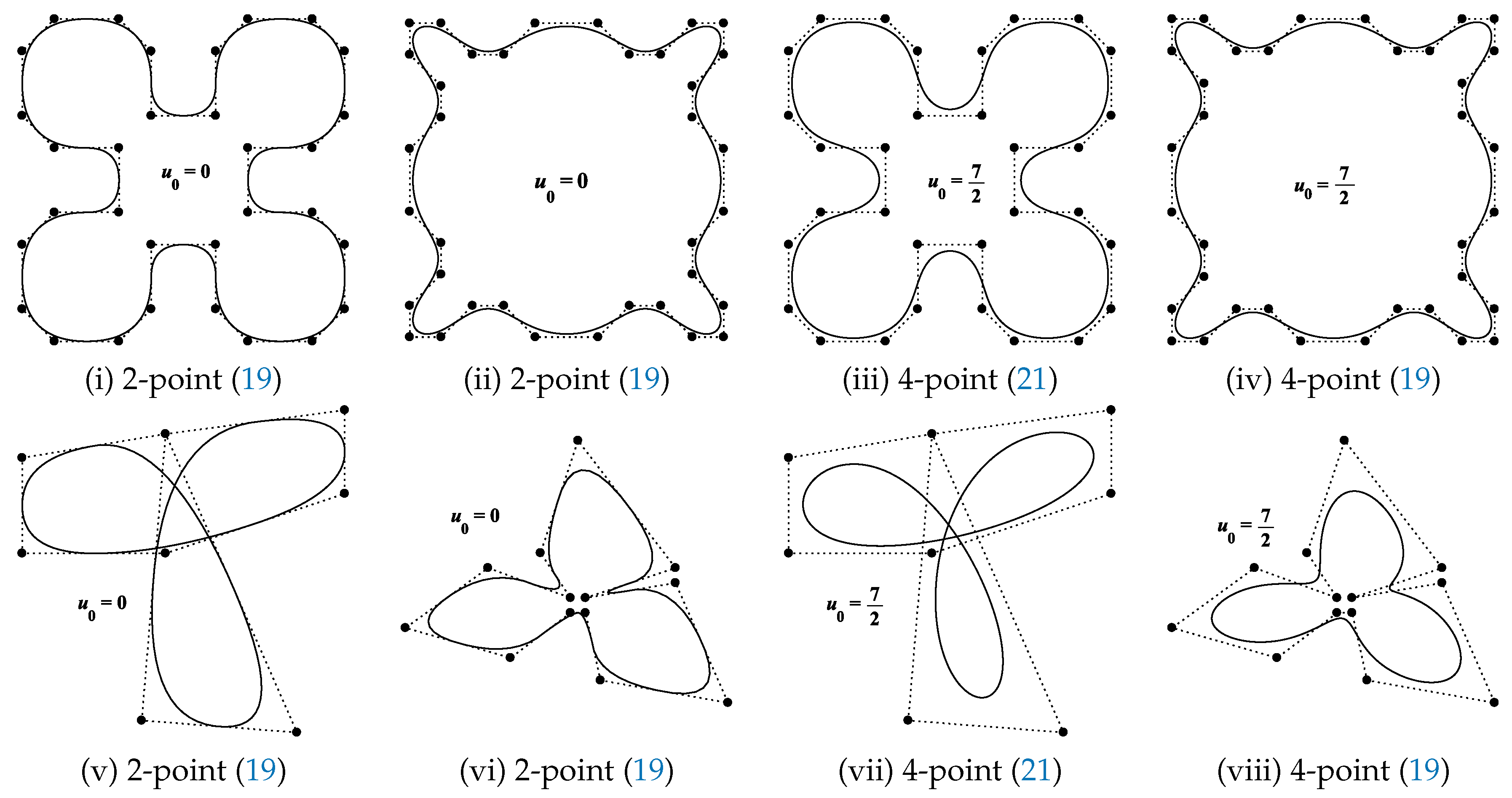
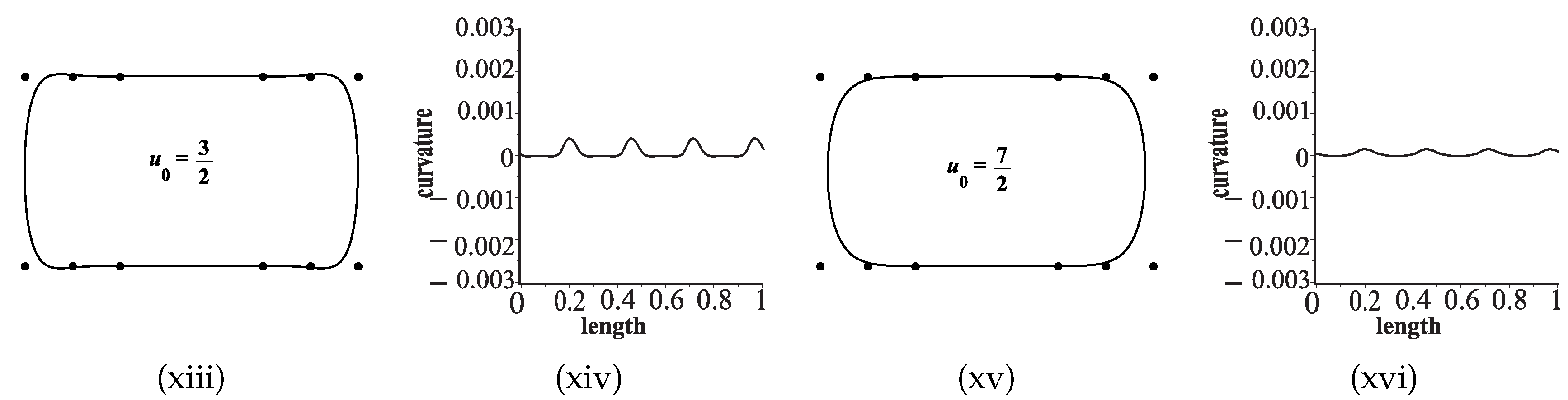
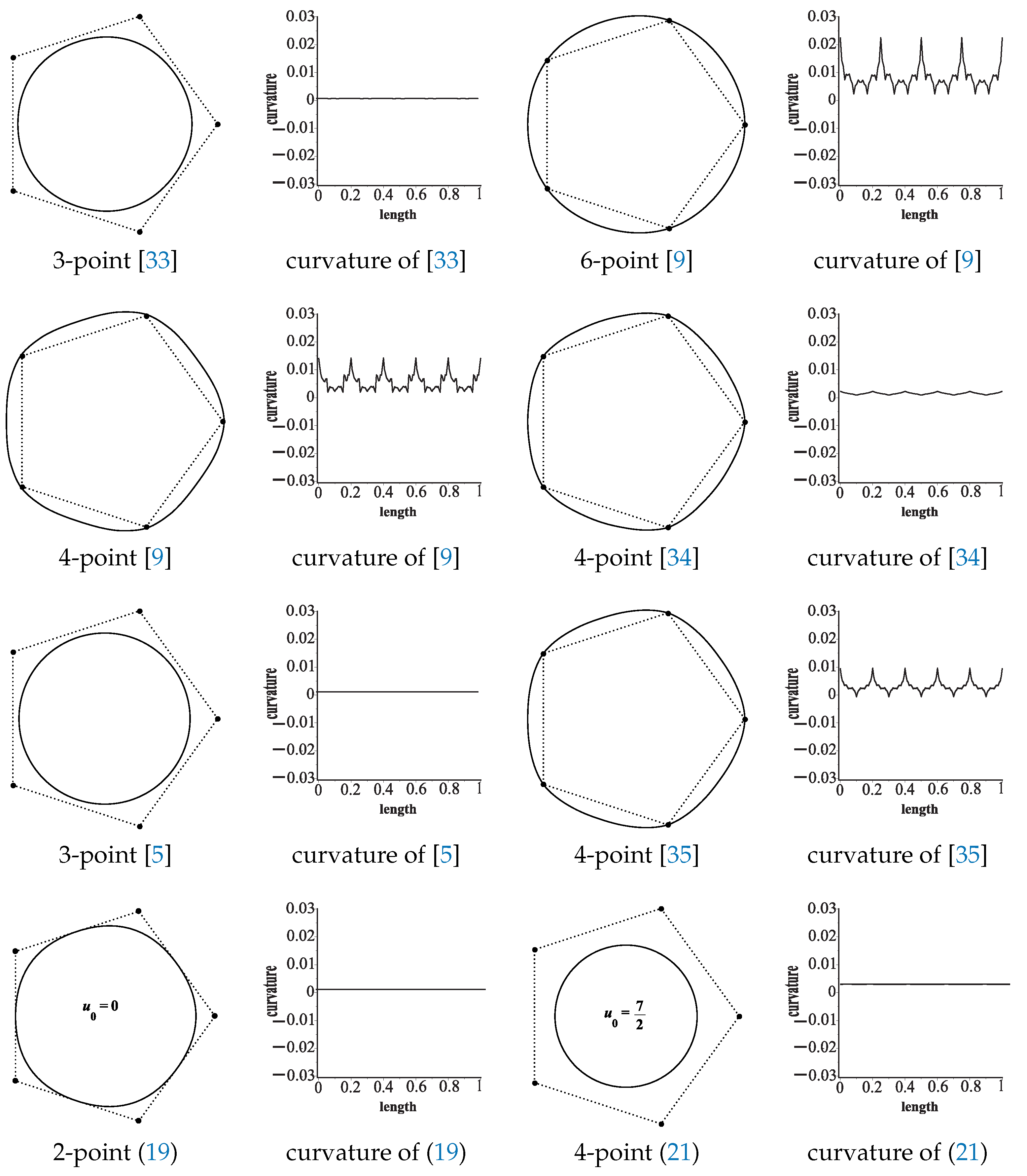
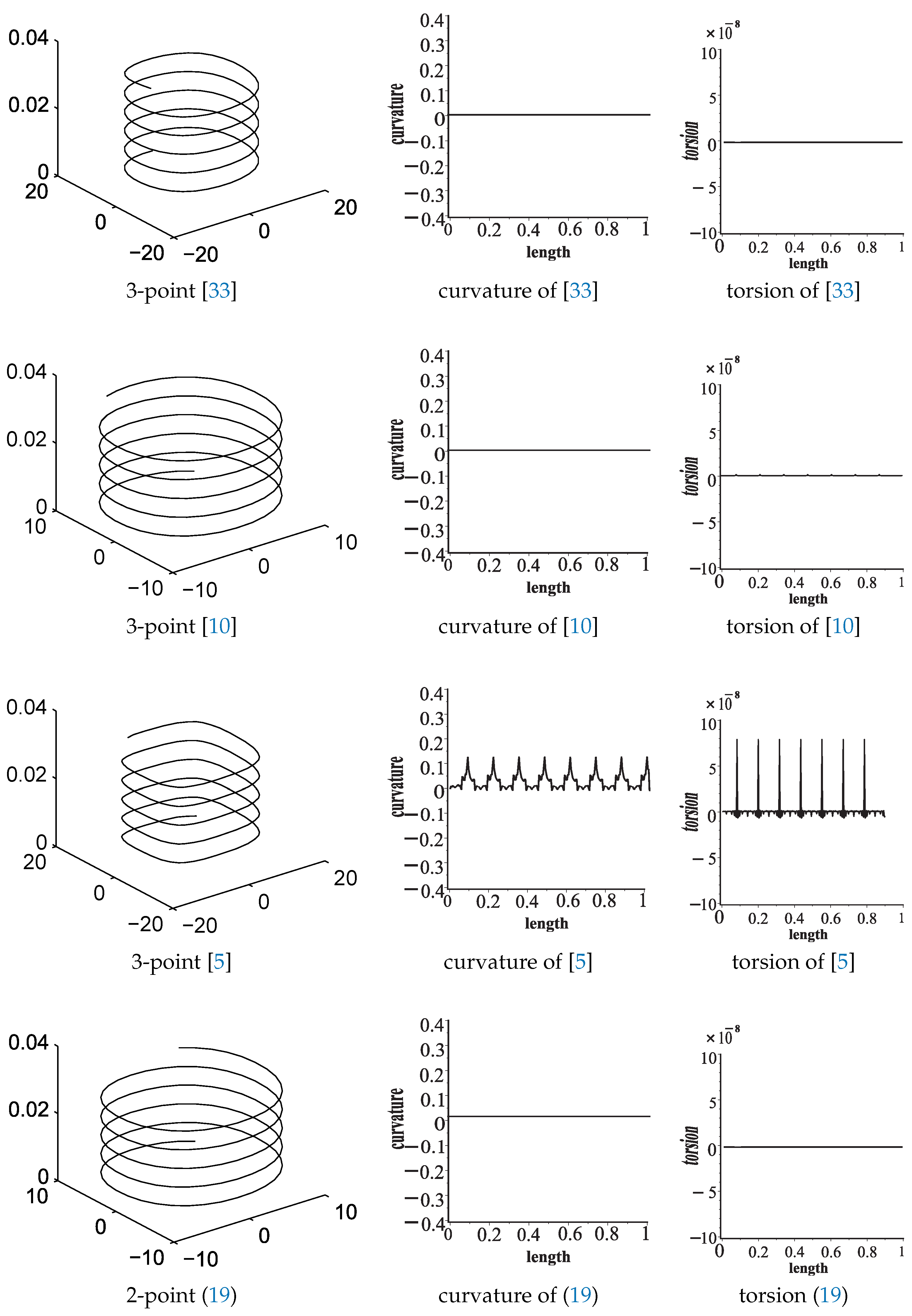
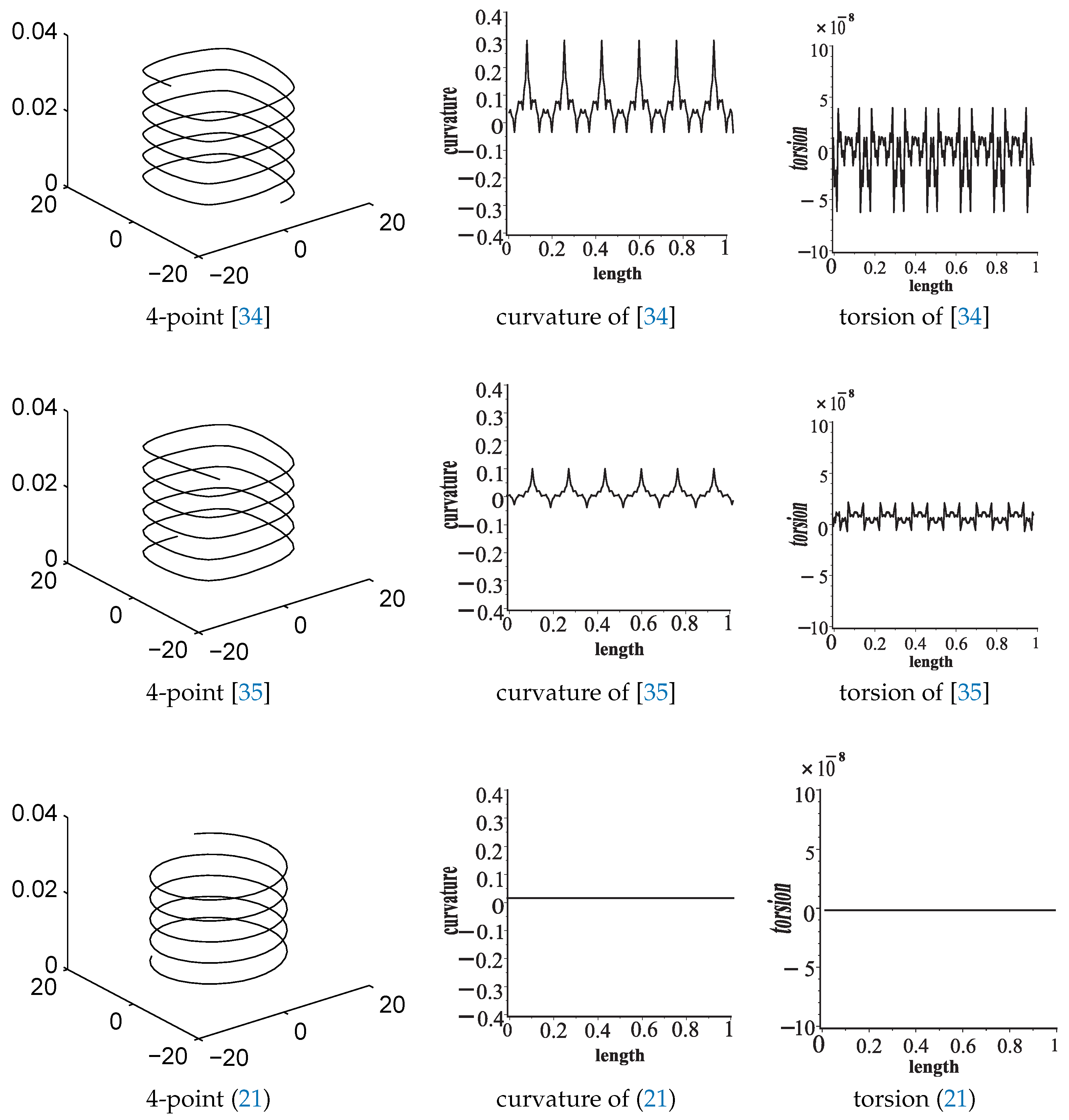
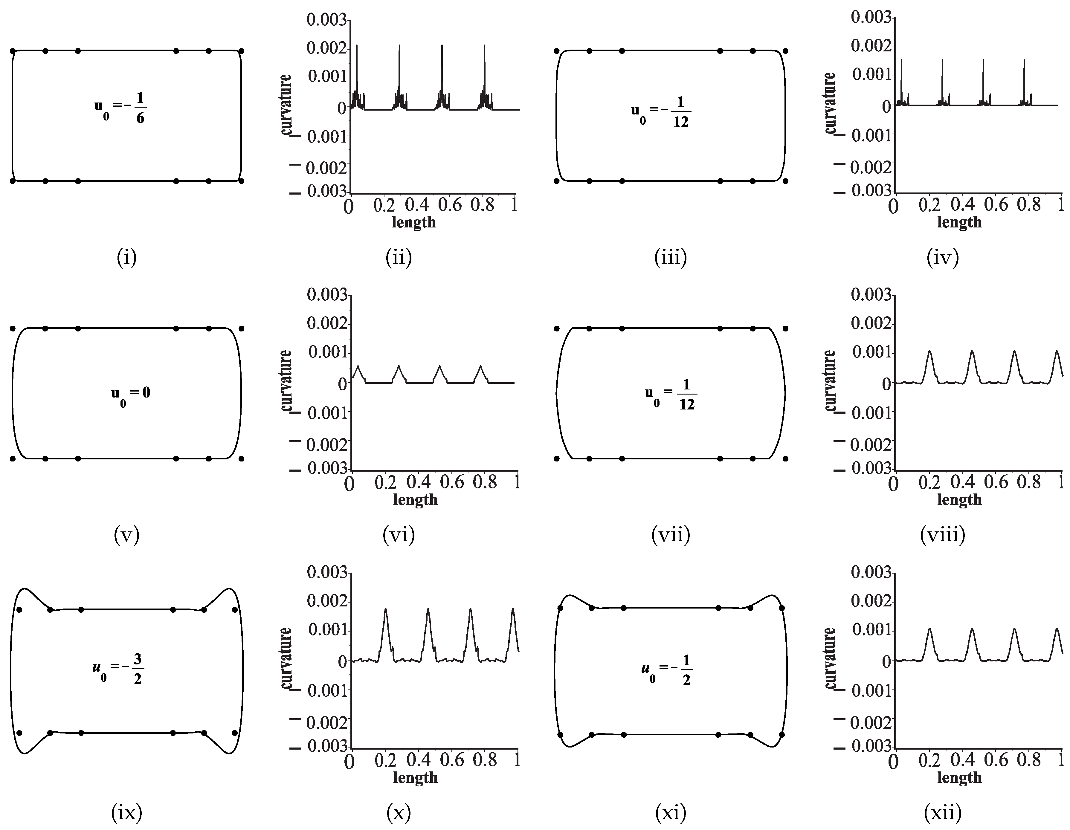
• Figure 1 demonstrates the visual performance of the proposed ANSSs. The limit curves, obtained by our ANSSs, are more rational as compared to other famous existing NSSs. In Figure 2, two examples are given to illustrate the behavior of the parameter $u_0$. The proposed ANSSs gives considerable variations in the results, which is a useful mechanism in geometric modeling.
• In Figure 3, five initial points are sampled to generate limit circle along with curvature. The limit curves generated by NSSs (19) and (21) Reference [5,9] have less tendency to depart from their tangent compared to the limit curves produced by [33,34,35].
• Figure 4 and Figure 5 indicate that curvature and torsion behavior of limit curves are closely related.

It is clear from the above comparison that the basic properties of limit curves generated by our proposed NSSs with a smaller number of initial control points have little tendency to depart from their tangents as well as their osculating planes compared to the limit curves obtained by the existing SSSs.

6. Conclusions and Future Research

Here, we have established an algorithm for the construction of even-point binary ANSS (for any integer $n\ge 1$) by using Lagrange-like interpolant. It is observed that the newly generated schemes by our proposed algorithm are a nonstationary counterpart of the SSs [2,5,24,30,31,32,34]. Moreover, in comparison with the schemes that have already emerged [5,9,10,33,34,35], the newly generated schemes are more refined and better in the sense of smoothness, curvature, and torsion. As observed, the proposed algorithm for different values of q can be considered more universal because it allows us to present general formulae for binary NSSs. These advantages motivate us to extend the proposed results in subdivision surface modeling.

References

1. De Rham, G. Sur une courbe plane. J. Math. Pures Appl. 1956, 35, 25–42. [Google Scholar]
2. Chaikin, G.M. An algorithm for high-speed curve generation. Comput. Graph. Image Process. 1974, 3, 346–349. [Google Scholar] [CrossRef]
3. Deslauriers, G.; Dubuc, S. Symmetric iterative interpolation processes. Constr. Approx. 1989, 5, 49–68. [Google Scholar] [CrossRef]
4. Dyn, N.; Levin, D. Stationary and non-stationary binary subdivision scheme. In Mathematical Methods in Computer Aided Geometric Design II; Lyche, T., Schumaker, L.L., Eds.; Academic Press: New York, NY, USA, 1992; pp. 209–216. [Google Scholar]
5. Jena, M.K.; Shunmugaraj, P.; Das, P.C. A subdivision algorithm for trigonometric spline curves. Comput. Aided Geom. Des. 2002, 19, 71–88. [Google Scholar] [CrossRef]
6. Wallner, J.; Dyn, N. Convergence and C1 analysis of subdivision schemes on manifolds by proximity. Comput. Aided Geom. Des. 2005, 22, 593–622. [Google Scholar] [CrossRef]
7. Beccari, C.; Casciola, G.; Romani, L. A nonstationary uniform tension controlled interpolating 4-point scheme reproducing conics. Comput. Aided Geom. Des. 2007, 24, 1–9. [Google Scholar] [CrossRef]
8. Beccari, C.; Casciola, G.; Romani, L. An interpolating 4-point C2 ternary non- stationary subdivision scheme with tension control. Comput. Aided Geom. Des. 2007, 24, 210–219. [Google Scholar] [CrossRef]
9. Daniel, S.; Shunmugaraj, P. An interpolating 6-point C2 non-stationary subdivision scheme. J. Comput. Appl. Math. 2009, 230, 164–172. [Google Scholar] [CrossRef]
10. Daniel, S.; Shunmugaraj, P. Three point stationary and non-stationary subdivision schemes. In Proceedings of the 3rd International Conference on Geometric Modeling & Imaging, London, UK, 9–11 July 2008. [Google Scholar] [CrossRef]
11. Conti, C.; Romani, L. A new family of interpolatory non-stationary subdivision schemes for curve design in geometric modeling. In Proceedings of the International Conference of Numerical Analysis and Applied Mathematics, Rhodes, Greece, 19–25 September 2010. [Google Scholar] [CrossRef]
12. Dyn, N.; Floater, M.S.; Hormann, K. Four-point curve subdivision based on iterated chordal and centripetal parameterizations. Comput. Aided Geom. Des. 2009, 26, 279–286. [Google Scholar] [CrossRef]
13. Li, B.-J.; Yu, Z.-L.; Yu, B.-W.; Su, Z.-X.; Liu, X.-P. Non-stationary subdivision for exponential polynomials reproduction. Acta Math. Appl. Sin. Engl. Ser. 2013, 29, 567–578. [Google Scholar] [CrossRef]
14. Siddiqi, S.S.; Younis, M. Ternary approximating non-stationary subdivision schemes for curve design. Cent. Eur. J. Eng. 2014, 4, 371–378. [Google Scholar] [CrossRef] [Green Version]
15. Conti, C.; Dyn, N.; Manni, C.; Mazure, M.L. Convergence of univariate non-stationary subdivision schemes via asymptotic similarity. Comput. Aided Geom. Des. 2015, 37, 1–8. [Google Scholar] [CrossRef]
16. Salam, W.; Siddiqi, S.S.; Rehan, K. Chaikins perturbation subdivision scheme in non-stationary forms. Alex. Eng. J. 2016, 55, 2855–2862. [Google Scholar] [CrossRef]
17. Tan, J.; Sun, J.; Tong, G. A non-stationary binary three-point approximating subdivision scheme. Appl. Math. Comput. 2016, 276, 37–43. [Google Scholar] [CrossRef]
18. Hameed, R.; Mustafa, G. Family of a-point b-ary subdivision schemes with bell-shaped mask. Appl. Math. Comput. 2017, 309, 289–302. [Google Scholar] [CrossRef]
19. Zhang, L.; Ma, H.; Tang, S.; Tan, J. A combined approximating and interpolating ternary 4-point subdivision scheme. J. Comput. Appl. Math. 2018, 350, 37–49. [Google Scholar] [CrossRef]
20. Ghaffar, A.; Ullah, Z.; Bari, M.; Nisar, K.S.; Baleanu, D. Family of odd point non-stationary subdivision schemes and their applications. Adv. Differ. Equ. 2019, 1, 171. [Google Scholar] [CrossRef]
21. Akram, G.; Bibi, K.; Rehan, K.; Siddiqi, S.S. Shape preservation of 4-point interpolating non-stationary subdivision scheme. J. Comput. Appl. Math. 2017, 319, 480–492. [Google Scholar] [CrossRef]
22. Mustafa, G.; Ghaffar, A.; Khan, F. The Odd-Point Ternary Approximating Schemes. Am. J. Comput. Math. 2011, 1, 111–118. [Google Scholar] [CrossRef] [Green Version]
23. Mustafa, G.; Ghaffar, A.; Aslam, M. A subdivision-regularization framework for preventing over fitting of data by a model. Appl. Appl. Math. Int. J. 2013, 8, 178–190. [Google Scholar]
24. Mustafa, G.; Khan, F.; Ghaffar, A. The m-point approximating subdivision scheme. Lobachevskii J. Math. 2009, 30, 138–145. [Google Scholar] [CrossRef]
25. Barton, M.; Shi, L.; Kilian, M.; Wallner, J.; Pottmann, H. Circular arc snakes and kinematic surface generation. Comput. Graph. Forum 2013, 32, 1–10. [Google Scholar] [CrossRef]
26. Song, X.; Aigner, M.; Chen, F.; Jüttler, B. Circular spline fitting using an evolution process. J. Comput. Appl. Math. 2009, 231, 423–433. [Google Scholar] [CrossRef] [Green Version]
27. Aslam, M.; Mustafa, G.; Ghaffar, A. The (2n−1)-point ternary approximating and interpolating subdivision schemes. J. Appl. Math. 2011, 2011, 13. [Google Scholar] [CrossRef]
28. Ghaffar, A.; Mustafa, G. The family of even-point ternary approximating schemes. ISRN Appl. Math. 2012, 1, 1–14. [Google Scholar] [CrossRef]
29. Dyn, N.; Levin, D. Analysis of asymptotically equivalent binary subdivision schemes. J. Math. Anal. Appl. 1995, 193, 594–621. [Google Scholar] [CrossRef]
30. Dyn, N.; Levin, D. Subdivision scheme in geometric modelling. Acta Numer. 2002, 11, 73–144. [Google Scholar] [CrossRef]
31. Siddiqi, S.S.; Ahmad, N. An approximating C4 stationary subdivision scheme. Eur. J. Sci. Res. 2006, 15, 97–102. [Google Scholar]
32. Zheng, H.; Hu, M.; Peng, G. P-ary subdivision seneralizing B-splines. In Proceedings of the 2009 Second International Conference on Computer and Electrical Engineering (ICCEE 2009), Dubai, UAE, 28–30 December 2009. [Google Scholar] [CrossRef]
33. Daniel, S.; Shunmugaraj, P. An approximating C2 non-stationary subdivision scheme. Comput. Aided Geom. Des. 2009, 26, 810–821. [Google Scholar] [CrossRef]
34. Daniel, S.; Shunmugaraj, P. Some interpolating non-stationary subdivision schemes. In Proceedings of the 2011 International Symposium on Computer Science and Society, Kota Kinabalu, Malaysia, 16–17 July 2011. [Google Scholar] [CrossRef]
35. Jena, M.K.; Shunmugaraj, P.; Das, P.C. A non-stationary subdivision scheme for curve interpolation. ANZIAM J. 2003, 44, 216–235. [Google Scholar] [CrossRef]
Figure 1. Four subdivision levels of SSs (19) and (21) have been used to the control polygon when control points are moved over a short distance, respectively.
Mathematics 07 00639 g001
Figure 2. Four subdivision levels of SS (19) and (21) have been used to the control polygon. The results after different values of u 0 are shown on the left together with their corresponding curvature on the right.
Mathematics 07 00639 g002aMathematics 07 00639 g002b
Figure 3. Comparison of existing and our proposed SS when five control points are sampled from circle. Limit curves obtained after 5th iteration are shown in the left column, the corresponding curvatures are shown in the right column.
Mathematics 07 00639 g003
Figure 4. Results of 5th iteration of the 3-point schemes [5,10,33] and (19) are shown on the left when the initial control points are sampled from Helix. The corresponding curvatures and torsions are shown in the center and right column, respectively.
Mathematics 07 00639 g004
Figure 5. Results of 5th iteration of the 4-point and 5-point schemes of [34,35] and (21) are shown on the left when the initial control points are sampled from Helix. The corresponding curvatures and torsions are shown in the center and right column, respectively.
Mathematics 07 00639 g005