Non-Parametric Threshold Estimation for the Wiener–Poisson Risk Model

Abstract

In this paper, we consider the Wiener–Poisson risk model, which consists of a Wiener process and a compound Poisson process. Given the discrete record of observations, we use a threshold method and a regularized Laplace inversion technique to estimate the survival probability. In addition, we also construct an estimator for the distribution function of jump size and study its consistency and asymptotic normality. Finally, we give some simulations to verify our results.

1. Introduction

Let $S={\left\{S_t\right\}}_{t\ge 0}$ with $S_0=0$ be a compound Poisson process defined as

$$\begin{array}{c}\hfill S_t={\displaystyle \sum _{i=1}^{N_t}}{\gamma }_i,t\ge 0,\end{array}$$

where ${\left\{N_t\right\}}_{t\ge 0}$ is a Poisson process with unknown intensity $\lambda >0$, and ${\gamma }_1,{\gamma }_2,{\gamma }_3,\dots$ are independent and identically distributed positive sequence of random variables with unknown distribution function F supported on $(0,\infty )$.

The Wiener–Poisson risk process is defined by

$$X_t=x+ct+\sigma W_t-{\displaystyle \sum _{i=1}^{N_t}}{\gamma }_i,t\ge 0,$$

(1)

where x is a given positive constant, $\sigma >0$ is an unknown constant, the corresponding process $\{N_t,t\ge 0\}$ is called the claim number process, ${\left\{{\gamma }_i\right\}}_{i=1,2,\dots }$ is a sequence of claims, and ${\left\{W_t\right\}}_{t\ge 0}$ is a standard Brownian motion. Suppose that ${\left\{N_t\right\}}_{t\ge 0}$, ${\left\{W_t\right\}}_{t\ge 0}$ and ${\left\{{\gamma }_i\right\}}_{i=1,2,\dots }$ are independent of each other, and the mean and variance of claim are finite, i.e., ${\mu }_{\gamma }={\int }_0^{\infty }xF\left(dx\right)<\infty$, ${\sigma }_{\gamma }^2={\int }_0^{\infty }{x}^{2}F\left(dx\right)-{\mu }_{\gamma }^2<\infty$. Further, we assume that the risk model in Equation (1) has a relative safety loading $\omega =\frac{c}{\lambda {\mu }_{\gamma }}-1>0$. Let $\tau \left(x\right)=inf\{t>0;X_t\le 0,X_0=x\}$. The survival probability of the risk model in Equation (1) is defined by:

$$\begin{array}{c}\hfill \Phi \left(x\right)=\mathbf{P}\left(\tau \left(x\right)=\infty \right),\end{array}$$

(2)

and $\Psi \left(x\right)=1-\Phi \left(x\right)$, the probability of ruin.

In the last few decades, many works have been contributed to the survival probability for the risk model in Equation (1) and its extended risk model. In [1], the author first introduced the risk model in Equation (1) and established an asymptotic estimate for $\Psi \left(x\right)$. In [2], the authors showed that $\Phi \left(x\right)$ satisfies a defective renewal equation. By renewal theory, they obtained the Pollaczeck–Khinchin formula of $\Phi \left(x\right)$. Accurate calculation and approximation for $\Psi \left(x\right)$ has always been an inspiration and an important source of technological development for actuarial mathematics (see, e.g., [3,4,5,6,7,8,9]). Although various approximations to the probability of ruin (e.g., importance sampling or saddle-point approximations) are now available, developing alternative approximations of different nature is still an interesting and practical problem.

In recent years, many authors studied the ruin probability by using statistical methods (see, e.g., [10,11,12,13,14,15,16,17,18]). In [17], the author assumed that $\left\{X_{t_i^n}\right|t_i^n=i{h}_n;i=0,1,2,\dots ,n\}$ and $\{{\gamma }_1,{\gamma }_2,\dots ,{\gamma }_{N_{t_n^n}}\}$ are observed, where $h_n=t_i^n-t_{i-1}^n$ is the sampling interval and the time of claims are known. The author constructed an estimator for Gerber–Shiu function and obtained its asymptotic property. Please refer to Equation (1.2) in [17] for the details of Gerber–Shiu function.

In our work, we suppose that a sample $\{X_{t_1^n},X_{t_2^n},X_{t_3^n},\dots ,X_{t_n^n}\}$ can be observed, where $h_n=t_i^n-t_{i-1}^n$ is the sampling interval. However, we cannot observe the exact time and size of claims. To estimate $\Phi \left(x\right)$, we have to estimate F, $\lambda$, $\lambda {\mu }_{\gamma }$ and ${\sigma }^2$. Given the discrete record of observations, we need to judge whether a claim occurs in the interval $(t_{i-1}^n,t_i^n]$. The threshold method from [19,20,21,22] is to determine that a single jump has occurred within $(t_{i-1}^n,t_i^n]$ if and only if the increment $|{\Delta }_{i}X|=|X_{t_i^n}-X_{t_{i-1}^n}|$ is larger than a suitable threshold function. By the threshold method and the work in [21,22], we can estimate F, $\lambda$, ${\mu }_{\gamma }$ and ${\sigma }^2$.

In [14,17], the authors estimated the ruin probability and Gerber–Shiu function by a regularized Laplace inversion technique. Using the threshold method and the work in [23], it is easy to obtain an estimator for the Laplace transform of $\Phi \left(x\right)$. To estimate $\Phi \left(x\right)$, the regularized Laplace inversion technique is used. Finally, we also obtain a rate of convergence for the estimator of $\Phi \left(x\right)$ in a sense of the integrated squared error (ISE).

This paper is organized as follows. In Section 2, we give some estimators for ${\sigma }^2$, $\lambda {\mu }_{\gamma }$, $\lambda$, F and its Laplace–Stieltjes transform. In Section 3, we study the asymptotic properties for the estimators. Finally, we give some conclusions in Section 5. All the technical proofs are presented in Appendix A.

2. Estimation of Survival Probability

To give the estimators for ${\sigma }^2$, $\lambda {\mu }_{\gamma }$, $\lambda$, F and the Laplace transform of F, we introduce the following filter:

$$\begin{array}{c}\hfill {\mathcal{C}}_i^n\left(\vartheta \left(h_n\right)\right)=\{\omega \in \Omega ;|{\Delta }_{i}X\left(\omega \right)|>\vartheta \left(h_n\right)\},\end{array}$$

(3)

where $\vartheta \left(h_n\right)$ is a threshold function and ${\mathcal{D}}_i^n\left(\vartheta \left(h_n\right)\right)$ is a complement of ${\mathcal{C}}_i^n\left(\vartheta \left(h_n\right)\right)$. In [19,20], the threshold function $\vartheta \left(h_n\right)$ satisfies ${lim}_{h_n\to 0}\vartheta \left(h_n\right)=0$ and ${lim}_{h_n\to 0}\frac{\sqrt{h_{n}log\left(\frac{1}{h_n}\right)}}{\vartheta \left(h_n\right)}=0$. In [21], the author gave an expression of threshold function $\vartheta \left(h_n\right)=L{h}_n^b$, where $L>0$ is a constant and $b\in (0,\frac{1}{2})$. Obviously, the expression of $\vartheta \left(h_n\right)$ from [21] satisfies the two conditions. In our work, the expression of $\vartheta \left(h_n\right)$ is similar to that in [21].

We first estimate F. Using $\left\{\right|{\Delta }_{i}X|;0\le i\le n,{\mathbf{I}}_{{\mathcal{C}}_i^n\left(\vartheta \left(h_n\right)\right)}=1\}$ and empirical distribution function, we can try to construct an estimator of F as follows:

$${\widehat{F}}_n\left(u\right)=\frac{1}{{\sum }_{i=1}^n{\mathbf{I}}_{{\mathcal{C}}_i^n\left(\vartheta \left(h_n\right)\right)}}{\displaystyle \sum _{i=1}^n}{\mathbf{I}}_{\left\{\right|{\Delta }_{i}X|\le u\}}{\mathbf{I}}_{{\mathcal{C}}_i^n\left(\vartheta \left(h_n\right)\right)},u\ge 0.$$

(4)

By Equations (3.4) and (3.6) in [21], the estimators of ${\sigma }^2$ and $\lambda$ are

$${\widetilde{{\sigma }^2}}_n=\frac{{\sum }_{i=1}^n{|{\Delta }_{i}X-c{h}_n|}^2{\mathbf{I}}_{{\mathcal{D}}_i^n\left(\vartheta \left(h_n\right)\right)}}{T_n},{\tilde{\lambda }}_n=\frac{{\sum }_{i=1}^n{\mathbf{I}}_{{\mathcal{C}}_i^n\left(\vartheta \left(h_n\right)\right)}}{T_n}.$$

By Equation (3.10) in [21], an estimator of $\lambda {\mu }_{\gamma }$ is given by

$${\widetilde{\lambda {\mu }_{\gamma }}}_n=\frac{{\sum }_{i=1}^n\left|{\Delta }_{i}X\right|{\mathbf{I}}_{{\mathcal{C}}_i^n\left(\vartheta \left(h_n\right)\right)}}{T_n}.$$

Let $\rho =\frac{\lambda {\mu }_{\gamma }}{c}$. Obviously, the estimator of $\rho$ is given by

$${\tilde{\rho }}_n=\frac{1}{c}\frac{{\sum }_{i=1}^n\left|{\Delta }_{i}X\right|{\mathbf{I}}_{{\mathcal{C}}_i^n\left(\vartheta \left(h_n\right)\right)}}{T_n}.$$

The Laplace transform of F is defined by $l_F=E\left[e^{-s{\gamma }_1}\right]={\int }_0^{\infty }{e}^{-su}F\left(du\right)$. An estimator of $l_F$ is given by

$${\widetilde{l_F}}_n\left(s\right)=\frac{{\sum }_{i=1}^n{e}^{-s|{\Delta }_{i}X|}{\mathbf{I}}_{{\mathcal{C}}_i^n\left(\vartheta \left(h_n\right)\right)}}{{\sum }_{i=1}^n{\mathbf{I}}_{{\mathcal{C}}_i^n\left(\vartheta \left(h_n\right)\right)}},$$

where $s\in \mathbb{E}$ and $\mathbb{E}$ is a compact subset of $(0,\infty )$.

By the work in [23], the Laplace transform of $\Phi \left(x\right)$ can be obtained as follows:

$$\begin{array}{ccc}\hfill L_{\Phi }\left(s\right)& =& {\int }_0^{\infty }{e}^{-sx}\Phi \left(x\right)dx\hfill \\ & =& \frac{1-\rho }{D\left(s\right)},s>0\hfill \end{array}$$

(5)

where $\rho =\frac{\lambda \mu }{c}$ and $D\left(s\right)=s+\frac{{\sigma }^2}{2c}{s}^2-\frac{\lambda }{c}(1-l_F\left(s\right))$.

Let us define an estimator of $L_{\Phi }\left(s\right)$ as follows:

$$\begin{array}{ccc}\hfill \widetilde{L_{\Phi }}\left(s\right)& =& \frac{1-{\tilde{\rho }}_n}{\tilde{D}\left(s\right)},\tilde{D}\left(s\right)=s+\frac{{\widetilde{{\sigma }^2}}_n}{2c}{s}^2-\frac{{\tilde{\lambda }}_n}{c}(1-{\widetilde{l_F}}_n\left(s\right)),s>0.\hfill \end{array}$$

(6)

To estimate $\Phi \left(x\right)$, we use the $L^2$-inversion method proposed from [24]. Now, we give the $L^2$-inversion method by Definition 1. We say that $f\in L^2(0,\infty )$ if $({\int }_0^{\infty }{\left|f\left(t\right)\right|}^2{dt)}^{\frac{1}{2}}<\infty$.

Definition 1.

Let$m>0$be a constant. The regularized Laplace inversion$L_m^{-1}:L^2(0,\infty )\to L^2(0,\infty )$is given by

$$\begin{array}{c}\hfill L_m^{-1}g\left(t\right)=\frac{1}{{\pi }^2}{\int }_0^{\infty }{\int }_0^{\infty }{\Psi }_m\left(y\right)y^{-\frac{1}{2}}{e}^{-tvy}g\left(v\right)dvdy\end{array}$$

(7)

for a function$g\in L^2(0,\infty )$and$t\in (0,\infty )$, where

$${\Psi }_m\left(y\right)={\int }_0^{a_m}cosh\left(\pi x\right)cos(xlogy)dx$$

and$a_m={\pi }^{-1}{cosh}^{-1}\left(\pi m\right)>0$.

For further information, and details of $L_m^{-1}$, please refer to [24].

To use Definition 1, it requires to verify $\widetilde{L_{\Phi }}\left(s\right)\in L^2(0,\infty )$. As n is sufficiently large, for $\mathbf{P}$-almost all $\omega \in \Omega$ and $s>0$, we have

$$\begin{array}{c}\hfill \mathbf{P}(\{\omega \in \Omega ;(1-{\tilde{\rho }}_n)s\le \tilde{D}\left(s\right)\le s+\frac{{\widetilde{{\sigma }^2}}_n}{2c}{s}^2\})=1.\end{array}$$

(8)

From Equations (6) and (8), it is obvious that $\widetilde{L_{\Phi }}\left(s\right)\notin L^2(0,\infty )$. The $L^2$-inversion method in Definition 1 cannot be applied at once.

Therefore, to use Definition 1, we have to amend $\widetilde{L_{\Phi }}\left(s\right)$.

Let

$$\begin{array}{c}\hfill {\Phi }_{\theta }\left(x\right)=e^{-\theta x}\Phi \left(x\right),x>0\end{array}$$

for arbitrary fixed $\theta >0$. It is obvious that

$$\begin{array}{c}\hfill L_{{\Phi }_{\theta }}\left(s\right)=L_{\Phi }(s+\theta ),s>0.\end{array}$$

An estimator of $L_{{\Phi }_{\theta }}$ is given by

$$\begin{array}{c}\hfill \widetilde{L_{{\Phi }_{\theta }}}\left(s\right)=\widetilde{L_{\Phi }}(s+\theta ),s>0.\end{array}$$

Obviously, $\widetilde{L_{{\Phi }_{\theta }}}\in L^2(0,\infty )$.

Finally, an estimator of $\Phi \left(x\right)$ is given by

$$\begin{array}{c}\hfill {\tilde{\Phi }}_{m\left(n\right)}\left(x\right)=e^{\theta x}\widetilde{{\Phi }_{\theta ,m\left(n\right)}}\left(x\right),x>0,\end{array}$$

(9)

where $\widetilde{{\Phi }_{\theta ,m\left(n\right)}}\left(x\right)=L_{m\left(n\right)}^{-1}\widetilde{L_{{\Phi }_{\theta }}}\left(s\right)$ and $m\left(n\right)>0$.

3. Asymptotic Properties

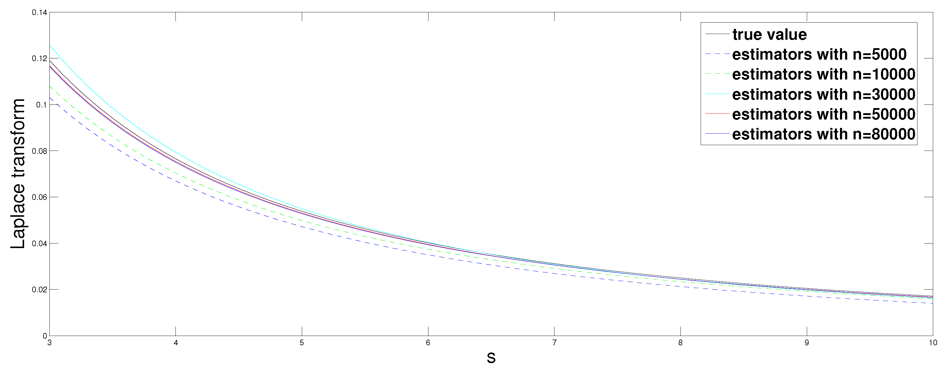
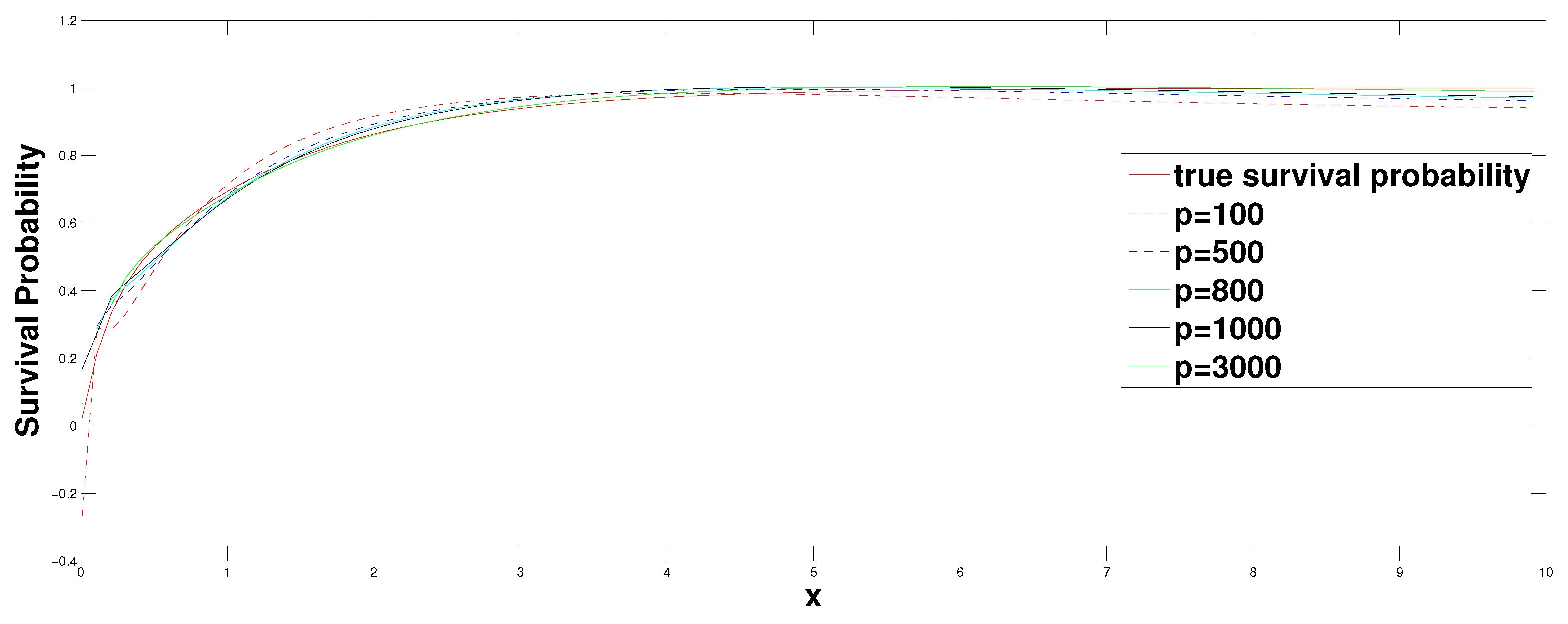
According to Theorem 3.1 in [19], the author assumed that $\sigma <Q$ and ${\gamma }_i\ge \Gamma$ with $Q>0$, $\Gamma >0$. In our work, Assumption 1 is used to prove the asymptotic properties of estimators.

Assumption A1.

There exist two positive constants Q and Γ such that$\sigma <Q$and$\mathbf{P}\left(\{\omega \in \Omega ;{\gamma }_i\ge \Gamma \}\right)=1$for$i=1,2,\dots$.

Let $\overline{F}=1-F$. With Equation (4), an estimator of $\overline{F}$ is given by

$$\begin{array}{ccc}\hfill {\overline{\widehat{F}}}_n\left(u\right)& =& \frac{1}{{\sum }_{i=1}^n{\mathbf{I}}_{{\mathcal{C}}_i^n\left(\vartheta \left(h_n\right)\right)}}{\displaystyle \sum _{i=1}^n}{\mathbf{I}}_{\left\{\right|{\Delta }_{i}X|>u\}}{\mathbf{I}}_{{\mathcal{C}}_i^n\left(\vartheta \left(h_n\right)\right)}.\hfill \end{array}$$

(10)

Let $\mathcal{N}(m,n)$ be a normal distribution with expectation m and variance n. Theorem 1 gives the asymptotic properties of ${\widehat{F}}_n\left(u\right)$.

Theorem 1.

Suppose that$T_n=n{h}_n\to \infty$, $n{h}_n^2\to 0$, $h_n\to 0$as$n\to \infty$and Assumption 1 is satisfied, then

$$\sqrt{T_n}\left({\overline{\widehat{F}}}_n\left(u\right)-\overline{F}\left(u\right)\right)\stackrel{\mathbf{D}}{\to }\mathcal{N}(0,\frac{\overline{F}\left(u\right)(1-\overline{F}\left(u\right))}{\lambda }).$$

(11)

Obviously,

$$\sqrt{T_n}\left({\widehat{F}}_n\left(u\right)-F\left(u\right)\right)\stackrel{\mathbf{D}}{\to }\mathcal{N}(0,\frac{F\left(u\right)(1-F(u\left)\right)}{\lambda }).$$

Remark 1.

By Dvoretzky–Kiefer–Wolfowitz inequality, we have

$$\mathbf{P}(\underset{u\in [0,\infty )}{sup}|{\widehat{F}}_n\left(u\right)-F\left(u\right)|>x)\le C{e}^{-2\lambda T_n{x}^2},x>0,$$

where C is a positive constant, not depending on F. Note that this inequality may be expression in the form:

$$\mathbf{P}(\sqrt{T_n}\underset{u\in [0,\infty )}{sup}|{\widehat{F}}_n\left(u\right)-F\left(u\right)|>x)\le C{e}^{-2\lambda x^2},x>0,$$

which clearly demonstrate that

$$\sqrt{T_n}\underset{u\in [0,\infty )}{sup}|{\widehat{F}}_n\left(u\right)-F\left(u\right)|=O_{\mathbf{P}}\left(1\right).$$

The asymptotic properties of ${\widetilde{{\sigma }^2}}_n$ are given by the following Lemma 1.

Lemma 1.

Suppose that$T_n=n{h}_n\to \infty$, $n{h}_n^2\to 0$and$h_n\to 0$as$n\to \infty$, then

$$\begin{array}{c}\hfill {\widetilde{{\sigma }^2}}_n\stackrel{\mathbf{P}}{\to }{\sigma }^2,n\to \infty .\end{array}$$

(12)

$$\begin{array}{c}\hfill \sqrt{n}({\widetilde{{\sigma }^2}}_n-{\sigma }^2)\stackrel{\mathbf{D}}{\to }\mathcal{N}(0,2{\sigma }^4),n\to \infty .\end{array}$$

(13)

Lemma 2.

Suppose that$T_n=n{h}_n\to \infty$, $n{h}_n^{\beta }\to 0$for some$\beta \in (1,2]$, $h_n\to 0$as$n\to \infty$and Assumption 1 is satisfied. Then,

$${\tilde{\lambda }}_n\stackrel{\mathbf{P}}{\to }\lambda ,\underset{\left\{s\right|s\in \mathbb{E}\}}{sup}|{\tilde{\lambda }}_n{\widetilde{l_F}}_n\left(s\right)-\lambda l_F\left(s\right)|\stackrel{\mathbf{P}}{\to }0,$$

(14)

$$\sqrt{T_n}({\tilde{\lambda }}_n-\lambda )\stackrel{\mathbf{D}}{\to }\mathcal{N}(0,\lambda ),$$

(15)

$${\tilde{\rho }}_n\stackrel{\mathbf{P}}{\to }\rho$$

(16)

and

$$\sqrt{n}({\tilde{\rho }}_n-\rho )\stackrel{\mathbf{D}}{\to }\mathcal{N}(0,\frac{\lambda {\sigma }^2}{c^2}),$$

(17)

as$n\to \infty$.

Let ${\parallel f\parallel }_B^2={\int }_0^B{\left|f\left(t\right)\right|}^{2}dt$ for any function f and $B>0$. Theorem 2 gives a rate of convergence for ${\tilde{\Phi }}_{m\left(n\right)}\left(x\right)$ in a sense of ISE.

Theorem 2.

Suppose that there exists a constant$K>0$such that$0\le {\Phi }^{\prime }\left(x\right)=g\left(x\right)\le K<\infty$and the conditions in Lemma 2 are satisfied. Then, for$m\left(n\right)=\sqrt{\frac{T_n}{log{T}_n}}$and for any constant$B>0$, we have

$$\parallel {\tilde{\Phi }}_{m\left(n\right)}{-\Phi \parallel }_B^2=O_P({(log{T}_n)}^{-1}),n\to \infty .$$

Remark 2.

The explicit expression for${\tilde{\Phi }}_{m\left(n\right)}\left(x\right)$is

$$\begin{array}{ccc}\hfill {\tilde{\Phi }}_{m\left(n\right)}\left(x\right)& =& \frac{e^{x\theta }}{{\pi }^2}{\int }_0^{\infty }{\int }_0^{\infty }{e}^{-xsy}\widetilde{L_{{\Phi }_{\theta }}}\left(s\right){\Psi }_{m\left(n\right)}\left(y\right)y^{-\frac{1}{2}}dsdy\hfill \end{array}$$

where${\Psi }_{m\left(n\right)}\left(y\right)={\int }_0^{a_{m\left(n\right)}}cosh\left(\pi x\right)cos(xlog\left(y\right))dx$and$a_{m\left(n\right)}={\pi }^{-1}{cosh}^{-1}\left(\pi m\left(n\right)\right)>0$and$m\left(n\right)=\sqrt{\frac{T_n}{log{T}_n}}$.

When c, λ, σ, F, θ,$\vartheta \left(h_n\right)$and sample size n are known,${\tilde{\Phi }}_{m\left(n\right)}\left(x\right)$can be evaluated with the command$integral2(f;0;\infty ;0;\infty )$of Matlab.

4. Simulation

If $F\left(x\right)=1-e^{-\frac{1}{{\mu }_{\gamma }}x}$, the survival probability is given by

$$\begin{array}{c}\hfill \Phi \left(x\right)=1-\frac{r_1+\frac{1}{{\mu }_{\gamma }}+\frac{2\lambda {\mu }_{\gamma }}{{\sigma }^2}}{r_1-r_2}{e}^{r_{1}x}-\frac{r_2+\frac{1}{{\mu }_{\gamma }}+\frac{2\lambda {\mu }_{\gamma }}{{\sigma }^2}}{r_2-r_1}{e}^{r_{2}x},x\ge 0,\end{array}$$

(18)

where $r_2<r_1<0$ are negative roots of the following equation

$$\begin{array}{c}\hfill \frac{1}{2}{\sigma }^{2}s+c-\frac{\lambda }{s+\frac{1}{{\mu }_{\gamma }}}=0.\end{array}$$

By the work in [25], Equation (18) is obtained easily.

Let $c=\lambda =10$, ${\mu }_{\gamma }=\frac{1}{2}$, $\sigma =5$, $\theta =0.075$, $\vartheta \left(h_n\right)=h_n^b$, $b=\frac{1}{4}$ and $h_n=n^{-\frac{4}{5}}$.

Firstly, we computed $\widetilde{L_{{\Phi }_{\theta }}}\left(s\right)$. In Figure 1, we plot the mean points with sample sizes $n=$ 5000, 10,000, 30,000, 50,000, 80,000, which were computed based on 5000 simulation experiments.

Figure 1. The estimator of ${\mathcal{L}}_{{\Phi }_{\theta }}$ with sample sizes $n=$ 5000, 10,000, 30,000, 50,000, 80,000.

In Remark 2, ${\tilde{\Phi }}_{m\left(n\right)}\left(u\right)$ is a double complex integrals. Using Matlab to compute ${\tilde{\Phi }}_{m\left(n\right)}\left(u\right)$ would take a long time. As shown in Figure 1, ${\widehat{\mathcal{L}}}_{{\Phi }_{\theta }}$ is very close to ${\mathcal{L}}_{{\Phi }_{\theta }}$ as $n\ge$ 30,000. To improve computational efficiency, let

$${\Phi }_p\left(x\right)=\frac{e^{x\theta }}{{\pi }^2}{\int }_0^{\infty }{\int }_0^{\infty }{e}^{-xsy}{[{\widehat{\mathcal{L}}}_{{\Phi }_{\theta }}\left(s\right)]}_{n=30000}{\Psi }_p\left(y\right)y^{-\frac{1}{2}}dsdy,$$

where ${[{\widehat{\mathcal{L}}}_{{\Phi }_{\theta }}\left(s\right)]}_{n=30000}=\frac{1-\frac{1}{c30000{\left(30000\right)}^{-\frac{4}{5}}}{\sum }_{k=1}^{30000}(c{\left(30000\right)}^{-\frac{4}{5}}-Z_k){\mathbf{I}}_{{\mathcal{D}}_k^{30000}}}{\frac{1}{c{\left(30000\right)}^{-\frac{4}{5}}}(\frac{1}{30000}{\sum }_{k=1}^{30000}{e}^{s{Z}_k}-1)}$, ${\Psi }_p\left(y\right)={\int }_0^{a_p}cosh\left(\pi x\right)cos(xlog\left(y\right))dx$ and $a_p={\pi }^{-1}{cosh}^{-1}\left(\pi p\right)>0$.

In Figure 2, we plot the mean points with sample sizes $n=$ 30,000 and $p=100,500,800,1000,3000$, which were computed based on 5000 simulation experiments.

Figure 2. ${\Phi }_p\left(x\right)$ with sample size $n=$ 30,000 and $p=100,500,800,1000,3000$.

5. Conclusions

In this paper, we use the threshold estimation technique and regularized Laplace inversion technique to constructed an estimator of survival probability for the Wiener–Poisson risk model. The rate of convergence for the estimator is a logarithmic rate. We adopt a method proposed by Cai et al. [26] to improve the speed in simulated calculation. The further work is to improve the speed of convergence for the estimator. We will combine the threshold estimation technique with Fourier transform (inversion) technique to construct an estimator of survival probability. We hope some further studies will be done when the risk model is the compound Poisson model with the barrier dividend strategy and investment. The Gerber–Shiu function and dividend function will be estimated by some statistical methods.

References

1. Gerber, H.U. An extension of the renewal equation and its application in the collective theory of risk. Scand. Actuar. J. 1970, 1970, 205–210. [Google Scholar] [CrossRef]
2. Dufresne, F.; Gerber, H.U. Risk theory for the compound Poisson process that is perturbed by diffusion. Insur. Math. Econ. 1991, 10, 51–59. [Google Scholar] [CrossRef]
3. Furrer, H.J.; Schimidli, H. Exponential inequalities for ruin probabilities of risk process perturbed by diffusion. Insur. Math. Econ. 1994, 15, 23–36. [Google Scholar] [CrossRef]
4. Gatto, R.; Mosimann, M. Four approaches to compute the probability of ruin in the compound Poisson risk process with diffusion. Math. Comput. Modell. 2012, 55, 1169–1185. [Google Scholar] [CrossRef]
5. Gatto, R.; Baumgartner, B. Saddlepoint Approximations to the Probability of Ruin in Finite Time for the Compound Poisson Risk Process Perturbed by Diffusion. Methodol. Comput. Appl. Probab. 2014, 18, 1–19. [Google Scholar] [CrossRef]
6. Gatto, R. Importance sampling approximations to various probabilities of ruin of spectrally negative Lévy risk processes. Appl. Math. Comput. 2014, 243, 91–104. [Google Scholar] [CrossRef]
7. Schimidli, H. Cramer-Lundberg approximations for ruin probabilites of risk processes perturbed by diffusion. Insur. Math. Econ. 1995, 16, 135–149. [Google Scholar] [CrossRef]
8. Veraverbeke, N. Asymptotic estimates for the probability of ruin in a Poisson model with diffusion. Insur. Math. Econ. 1993, 13, 57–62. [Google Scholar] [CrossRef]
9. Wang, Y.; Yin, C. Approximation for the ruin probabilities in a discrete time risk model with dependent risks. Stat. Probab. Lett. 2010, 80, 1335–1342. [Google Scholar] [CrossRef]
10. Bening, V.E.; Korolev, V.Y. Nonparametric estimation of the ruin probability for generalized risk processes. Theory Probab. Its Appl. 2002, 47, 1–16. [Google Scholar] [CrossRef]
11. Croux, K.; Veraverbeke, N. Non-parametric estimators for the probability of ruin. Insur. Math. Econ. 1990, 9, 127–130. [Google Scholar] [CrossRef]
12. Frees, E.W. Nonparametric estimation of the probability of ruin. Astin Bull. 1986, 16, 81–90. [Google Scholar] [CrossRef]
13. Hipp, C. Estimators and bootstrap confidence intervals for ruin probabilities. Astin Bull. 1989, 19, 57–70. [Google Scholar] [CrossRef]
14. Mnatsakanov, R.; Ruymgaart, L.L.; Ruymgaart, F.H. Nonparametric estimation of ruin probabilities given a random sample of claims. Math. Methods Stat. 2008, 17, 35–43. [Google Scholar] [CrossRef]
15. Pitts, S.M. Nonparametric estimation of compound distributions with applications in insurance. Ann. Inst. Stat. Math. 1994, 46, 537–555. [Google Scholar]
16. Politis, K. Semiparametric estimation for non-ruin probabilities. Scand. Actuar. J. 2003, 2003, 75–96. [Google Scholar] [CrossRef]
17. Shimizu, Y. Non-parametric estimation of the Gerber-Shiu function for the Wiener-Poisson risk model. Scand. Actuar. J. 2012, 2012, 56–69. [Google Scholar] [CrossRef]
18. Zhang, Z.; Yang, H. Nonparametric estimate of the ruin probability in a pure-jump lévy risk model. Insur. Math. Econ. 2013, 53, 24–35. [Google Scholar] [CrossRef]
19. Mancini, C. Estimation of the characteristics of the jump of a general Poisson-diffusion model. Scand. Actuar. J. 2004, 1, 42–52. [Google Scholar] [CrossRef]
20. Mancini, C. Non-parametric threshold estimation for models with stochastic diffusion coefficient and jumps. Scand. J. Stat. 2009, 36, 270–296. [Google Scholar] [CrossRef]
21. Shimizu, Y. A new aspect of a risk process and its statistical inference. Insur. Math. Econ. 2009, 44, 70–77. [Google Scholar] [CrossRef]
22. Shimizu, Y. Functional estimation for lévy measures of semimartingales with Poissonian jumps. J. Multivar. Anal. 2009, 100, 1073–1092. [Google Scholar] [CrossRef]
23. Morales, M. On the expected discounted penalty function for a perturbed risk process driven by a subordinator. Insur. Math. Econ. 2007, 40, 293–301. [Google Scholar] [CrossRef]
24. Chauveau, D.E.; Vanrooij, A.C.M.; Ruymgaart, F.H. Regularized inversion of noisy Laplace transforms. Adv. Appl. Math. 1994, 15, 186–201. [Google Scholar] [CrossRef]
25. Asmussen, S.; Albrecher, H. Ruin Probabilities, 2nd ed.; World Scientific: Singapore, 2010. [Google Scholar]
26. Cai, C.; Chen, N.; You, H. Nonparametric estimation for a spectrally negative Lévy process based on low–frequency observation. J. Comput. Appl. Math. 2018, 328, 432–442. [Google Scholar] [CrossRef]
Figure 1. The estimator of L Φ θ with sample sizes n = 5000, 10,000, 30,000, 50,000, 80,000.
Mathematics 07 00506 g001
Figure 2. Φ p ( x ) with sample size n = 30,000 and p = 100 , 500 , 800 , 1000 , 3000 .
Mathematics 07 00506 g002