Abstract
In this paper, a class of fractional complex networks with impulses and reaction–diffusion terms is introduced and studied. Meanwhile, a class of more general network structures is considered, which consists of an instant communication topology and a delayed communication topology. Based on the Lyapunov method and linear matrix inequality techniques, some sufficient criteria are obtained, ensuring adaptive pinning synchronization of the network under a designed adaptive control strategy. In addition, a pinning scheme is proposed, which shows that the nodes with delayed communication are good candidates for applying controllers. Finally, a numerical example is given to verify the validity of the main results.
1. Introduction
Complex networks, which are composed of a large set of nodes connected by edges, are used to describe many large-scale systems in nature and human societies, such as the Internet, power grid networks, the World Wide Web and so on [1,2,3]. Therefore, it is very meaningful and important to investigate the dynamical behaviors of complex networks. Up until now, there have been a large number of excellent scientific research results on the dynamical analysis of complex networks, including of synchronization [4], state estimation [5], impulsive control [6], and so on.
Synchronization, as one of the most important collective behaviors of complex dynamical systems, widely exists in the world, ranging from natural systems to man-made networks [7,8]. In recent years, synchronization has received a great deal of attention due to its potential application in various fields, including signal processing, secure communication, biological systems, and so on [9,10,11]. Various types of synchronization problems have been studied, such as projective lag synchronization [12], cluster synchronization [13], and exponential synchronization [14]. However, as we know, it is impossible for most dynamical systems to achieve synchronization by themselves in many real situations. Some control strategies must be designed to force the systems to be synchronized, such as feedback control [15], impulsive control [16], and adaptive control [17]. It could be a waste of money and resources op add controllers to all nodes in a large-scale network. In order to solve this problem, a pinning control strategy, which involves only a small fraction of all the nodes being controlled to force networks to become synchronized, has been proposed and extensively studied by researchers [18,19]. To reduce the enormous difference in control strength between theoretical values and practical needs, adaptive control, as a valid method, has been discussed in literature [20,21].
In practice, diffusion phenomena cannot be ignored. For example, electrons move in a nonuniform electromagnetic field and, in the process of chemical reactions, different chemicals react with each other and spatially diffuse in the inter-medium until a balanced-state spatial concentration pattern has been structured. Thus, it is reasonable to consider complex networks with reaction–diffusion terms. In recent years, some papers concerning the control and synchronization of complex dynamical systems with diffusion effects terms have been published [22,23,24]. In the real world, the state of artificial and biological networks are often subject to instantaneous perturbations and experience abrupt changes at certain instants, which may be caused by switching phenomena, frequency changes, or other sudden noises. These instantaneous perturbations always exhibit impulsive effects. Impulsive dynamical systems have naturally received a lot of attention, and some excellent results have been published [25,26]. Therefore, it is necessary to investigate the influence of impulsive perturbations on complex networks.
It should be noted that all of the mathematical models in this paper are fractional systems. As a generalization of traditional calculus, fractional calculus [27] provides an excellent instrument for the description of memory and the hereditary properties of various materials and processes. With the development of scientific research, these advantageous properties of fractional integration and differentiation have been noticed by more and more researchers, and fractional calculus, as a useful tool, has been widely applied in many fields such as mathematical biology [28], signal processing [29], and so on.
In addition, to be more practical, it is necessary to consider time delay. Due to the finite switching speed of amplifiers and the finite signal propagation time, time delay naturally exists in all kinds of dynamical systems and is unavoidable, which may lead to instability, chaos, or other performances of dynamical systems [30,31]. Thus, it is valuable to investigate the phenomenon of time delay in complex dynamical systems, and some outstanding results from research into time delay have been published, such as [32].
Motivated by the above discussions, the main contributions of this paper are as follows. (1) A class of fractional complex networks with impulses and reaction–diffusion terms is studied. Meanwhile, a class of more general network structures is considered in which all nodes are divided into three categories: nodes can only send information to others instantly; nodes can only be connected with others with a time delay; and nodes can communicate both instantly and with a delay. (2) Some sufficient conditions are derived to ensure the adaptive pinning synchronization of the network. (3) A pinning scheme is designed that shows that some delay-coupled nodes should be pinned first.
The rest of this paper is arranged as follows: some preliminaries and the model description of fractional networks with impulses and reaction–diffusion terms are provided in Section 2; in Section 3, the main results of this paper are described; next, in Section 4, a numerical simulation is presented to illustrate the effectiveness and correctness of the main results; finally, the conclusion of this paper is given in Section 5.
: Let , , be the n-dimensional Euclidean space, and be the space of real matrices. means that matrix P is symmetric and semi-positive (semi-negative) definite. means that matrix P is symmetric and positive (negative) definite. denotes an real identity matrix. is the transpose of matrix A. means the inverse of matrix B. Let where . ⊗ represents the Kronecker product of two matrices. and denote the minimum and the maximum eigenvalue of the corresponding matrix, respectively. denotes the Euclidean norm of a vector, for example, where .
2. Preliminaries and System Description
In this section, some basic definitions of fractional calculus are introduced as the preliminaries of this paper, and some necessary conclusions are presented for use in the next several sections. Meanwhile, the mathematical model of a class of fractional complex networks with impulses and reaction–diffusion terms is described and the definition of synchronization of complex networks is given.
2.1. Fractional Integral and Derivative
Definition 1
([33]). Riemann–Liouville fractional derivative with order α for a function is defined as
where , , and denotes the collection of all positive integers. is the gamma function.
Definition 2
([33]). Riemann–Liouville fractional integral of order α for a function is defined by
where and is the gamma function.
Lemma 1
([33]). For any constants and , the linearity of the Riemann–Liouville fractional derivative is described by
Lemma 2
([33]). If , then the following equality
holds for sufficiently good functions . In particular, this relation holds if is integrable.
Lemma 3
([34]). Let be a vector of differentiable function. Then, for any time instant , the following inequality holds
where and is a constant, square, symmetric, and positive definite matrix.
Lemma 4
([35]). Let Ω be a cube , and let be a real-valued function belonging to , which vanishes on the boundary of Ω, i.e., . Then,
where .
Lemma 5
([36]). The following linear matrix inequality
where and , is equivalent to any one of the following conditions:
Lemma 6
([37]). For any , , the inequality holds.
2.2. Theories of Graphs and Matrices
An undirected graph consists of nodes and a set of edges . If there is an edge between nodes i and j, then , and node j is called the neighbor of node i and vice versa. The Laplacian matrix representing the topological structure of graph is defined as: when , if ; otherwise, ; , which ensures the property that .
Lemma 7
([38]). If L is the Laplacian matrix of a connected network, for , and for all , then all eigenvalues of the matrix
are positive for any positive constant ε.
Lemma 8
([39]). For matrices A, B, C, and D with appropriate dimensions, the Kronecker product ⊗ satisfies
- (1)
- , where θ is a constant;
- (2)
- ;
- (3)
- ;
- (4)
- .
Lemma 9
([40]). The Laplacian matrix L in an undirected graph is semi-positive definite. It has a simple zero eigenvalue, and all the other eigenvalues are positive if and only if the graph is connected.
2.3. System Description
In this paper, a class of fractional complex networks with time-varying delays is considered. It is assumed that there exist two different modes of communication between the nodes in a network: instant communication and delayed communication. Namely, the network structure consists of two topologies, the instant communication topology and the delayed communication topology . and , where and denote the sets of instant communication links and delayed communication links, respectively. Let and represent the Laplacian matrices of and , respectively. It is noted that each node in the network has at least one mode of communication and that the graphs and can be disconnected, which implies that they consist of several connected components, and each component is considered as a cluster (group or family). In other words, if there are p nodes that can only communicate with other nodes instantly and q nodes that can only be connected to others with delays, then there exist two elementary matrices F and H such that
where and are the Laplacian matrices of the ith connected component of and , respectively. Then the mathematical model of fractional complex networks with impulses and reaction–diffusion terms is considered as follows:
where denotes the Riemann–Liouville fractional derivative operator of order ; , is the Laplace diffusion operator on ; is the state vector of the ith node at time t and in space x; , and is the transmission diffusion coefficient along the ith node; corresponds to the time-varying delay at time t, and it is a continuous function satisfying , , where and are nonnegative constants; is a continuously differentiable vector function; and are the coupling strength; and are positive semi-definite inner coupling matrices where if two nodes can communicate through the jth state and otherwise; and are the Laplacian matrices representing the topological structure of the network; denote impulsive moments and satisfy , , and ; and are the state variables of the ith node before and after impulsive perturbation, respectively; , , and assuming that , the solution of system is left continuous at time ; is the function of the change of at time in space x.
Next, the dynamics of an isolated node can be described by
where is the state vector of the isolated node and may be an equilibrium point, a periodic orbit, or even a chaotic orbit.
Synchronization errors between the relative state of nodes in network and the state of an isolated node can be defined by . Next, the definition of synchronization of complex networks is given as follows
Definition 3.
A complex network (2) is said to be synchronized if for any initial condition, the following equality is satisfied:
Remark 1.
The model (2) has been proposed and studied in [41,42]. But it is different from [41,42] in that impulsive perturbations, reaction–diffusion terms, and a class of more general network structures are considered in this paper. All nodes in the network can be divided into three categories: (1) nodes that can only send information to others instantly; (2) nodes that can only be connected to others with a time delay; and (3) nodes that can communicate with others both instantly and with a delay. Note that the assumption that the whole network should be connected is no longer needed. Thus, the mathematical model is more practical.
Remark 2.
The impulses in the system (2) can be understood as a special property of the system itself or some uncertain disturbances caused by external noises. The pulse period may be no longer fixed or regular, and the intensity of the impulses can be uncertain.
3. Main Results
In this section, some sufficient criteria for pinning and adaptive synchronization of complex networks (2) are derived, and a pinning scheme is given to discuss which node should be selected first.
Throughout this paper, the following assumptions are needed:
Assumption 1.
The set Ω is that where are positive constants.
Assumption 2.
There exist functions such that the functions satisfy
where , . stands for the impulsive strength of the ith node at time instants and in space x.
Assumption 3.
(One-sided Lipschitz condition) There exists a constant diagonal matrix such that
Remark 3.
Note that is very mild [43]. For example, all linear and piece-wise linear functions satisfy this condition. In addition, if are bounded, the above condition is satisfied in many well-known systems such as the Lorenz system, Chen system, L system, recurrent neural networks, Chua’s circuit, and so on. Generally speaking, any function in the system that satisfyies the Lipschitz condition can guarantee this assumption. According to [44], any Lipschitz function is a one-sided Lipschitz function, but the converse is not true. This means that for some nonlinear functions with a big Lipschitz constant, the corresponding one-sided Lipschitz constant matrix Ξ may be a non-positive definite matrix (see the example given in [45]).
3.1. Adaptive and Pinning Control
The boundary and initial value conditions of complex networks are given in the following form:
where , and is bounded and continuous on .
Then, the synchronization error system between systems (2) and (3) is given as follows:
where and are used above. is the n-dimensional linear feedback controller on the ith node. Without loss of generality, it is assumed that the first l nodes are controlled in the network, and the pinning controller is designed by
where denotes control gain.
Next, a theorem is established to derive the synchronization criteria for network (2).
Theorem 1.
Proof of Theorem 1.
Let where . Then, the proof of this theorem can be given in two steps.
Firstly, the case of and , is considered. According to Assumption 2, the following inequality holds:
where .
Secondly, the case of and is considered. Consider the following Lyapunov function for error system (6),
where and .
Taking the time derivative of along the trajectories of (6), it is evident that and are continuous when . Then, by Lemmas 2 and 3, the following inequality holds:
From Green’s formula and the boundary conditions, the following equality holds:
According to Lemma 4, the following inequality can be obtained:
By using Lemma 6, an inequality holds as follows:
where , and , .
Next, it can be proven that for and . Suppose, for the purpose of contradiction, that . According to the properties of function that and , there exists a positive constant such that for (monotone and bounded property). Thus, for . Then the following inequality holds:
where . This contradicts the previous hypothesis.
Remark 4.
According to Lemma 5, the matrix Q in (8) and (9) can be found by solving the linear matrix inequalities and . Furthermore, conditions (8) and (9) provide the control design for synchronization of network (2). It is easy to see that the coupling strengths c and play a key role in (8) and (9). If the coupling strengths c and can be designed, the larger c and the smaller can make these conditions easier to satisfy.
In order to reduce the enormous difference in control strength between theoretical values and practical need, adaptive and pinning control is considered. Then, without loss of generality, it is assumed that the first l nodes are controlled in the complex networks (2) and an adaptive pinning controller is designed by
where denote control strength.
Next, a theorem is obtained to guarantee that the complex networks (2) can be adaptively synchronized.
Theorem 2.
Proof of Theorem 2.
The proof of this theorem is given in two steps.
Firstly, the case of and , is considered. Similar to the proof of Theorem 1, the following conclusion can be obtained immediately:
Secondly, the case of and is considered. Consider the following Lyapunov function for error system (6),
where and , . are non-negative constants that should be determined later.
Similar to the proof of Theorem 1, computing the derivative of along the trajectories of error system (6) under the adaptive law and controller (19), the following inequality is obtained,
Then,
3.2. Pinning Scheme of Complex Networks
In order to design a pinning scheme for network (2), some notations are introduced for simplicity. Let
Using matrix decomposition, the following equation holds:
where . is obtained by removing the first l row–column pairs of matrix .
Then, a necessary condition is proposed to clearly reveal how the network’s characters can affect the pinning synchronization criteria.
Theorem 3.
Proof of Theorem 3.
According to Lemma 5, condition (8) is equivalent to . It is necessary that . □
Remark 5.
is an element of the Laplacian matrix , which denotes the delayed communication topology of network (2). According to the definition of the Laplacian matrix, the greater the degree of the ith node is, the greater the value of is, and vice versa. From (29) and (30), for the nodes without a controller, the degrees of these nodes in the delayed communication topology must be less than a critical value. Namely, the condition must be satisfied, which indicates that the nodes with large degrees in delayed communication topology should be controlled first, otherwise, (30) is not satisfied. This is consistent with the intuition that the delayed communication between nodes can lead to some instability in the network. In addition, some results have been proposed [43] that, in the instant communication topology network, nodes with very low and very large degrees are good candidates for applying pinning controllers.
In order to be more practical, some low-dimensional conditions are presented to guarantee the global asymptotic stability of the pinning process.
Theorem 4.
Remark 6.
Remark 7.
Note that for , the model of complex networks (2) reduces to the classical integer-order system with impulsive effects and reaction–diffusion terms. It is not difficult to verify that, in the case of , the conditions given in Theorems 1, 2, and 4 can also guarantee the synchronization of corresponding integer-order complex networks via the designed controllers (7) and (19). Therefore, the synchronization results in Theorems 1, 2, and 4 extend and improve the synchronization results for integer-order complex networks with reaction–diffusion terms and impulsive effects compared to the fractional case.
Remark 8.
When , the partial differential equations (2) can be degraded to fractional ordinary differential equations. It is easy to demonstrate that in this special case, the criteria given in Theorems 1, 2, and 4 are also valid for ensuring the synchronization of corresponding ordinary differential systems under controllers (7) and (19).
Remark 9.
In recent years, many outstanding results from the analysis of the stability of fractional systems, as in [46,47,48,49], have been reported. But, since there exists an integration term in the definition of the Riemann–Liouville fractional derivative, which means that the fractional derivative of a function at any given moment depends on its initial state, the existing fractional Lyapunov methods are invalid for analyzing the stability of fractional systems with impulsive effects. Thus, according to Lemma 2, two special Lyapunov functions with fractional integration terms are constructed to complete the proof of Theorems 1 and 2.
Remark 10.
Adaptive control for fractional complex networks (2) is studied in this paper. However, there is no such property of the Riemann–Liouville fractional derivative that for , where m is a constant. Therefore, an integer-order adaptive law (19) is designed rather than a fractional-order adaptive law. This is more practical because the computational complexity of fractional derivatives is much higher than that of integral derivatives.
4. Numerical Simulations
In this section, an example is given to illustrate the effectiveness of the main results.
Example 1.
Consider the two-dimensional Riemann–Liouville fractional complex network (2), which consists of five nodes, with impulses and reaction–diffusion terms. The parameters are designed as: ; , ; ; are identity matrices; , ; and the Laplacian matrices are given as follows:
The nonlinear function is
where . The boundary and initial value conditions of the isolated node (3) and network (2) are given in the form
where , , , , , . The impulsive strength functions are given as follows: , , , , , . The pulse period is .
Pinning control strategy is considered here, supposing the first node in network (2) is controlled. Then, the appropriate controller and adaptive law can be designed as follows:
where . and .
Let stand for the norm of synchronization error between systems (2) and (3). In Figure 1, Figure 2, Figure 3 and Figure 4, it is shown that under the adaptive law and designed controller (36), complex networks (2) with reaction–diffusion terms and impulsive effects can achieve synchronization. In Figure 5, it is easy to see that the adaptive control parameter turns out to be a constant , which satisfies the conditions in Theorem 2, when synchronization is realized. The efficiency of Theorem 2 can be demonstrated by this example.
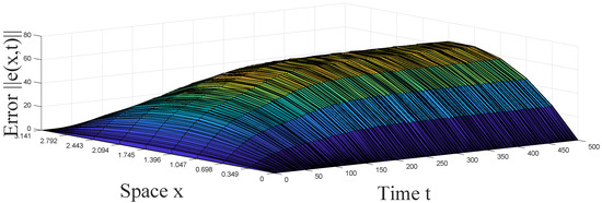
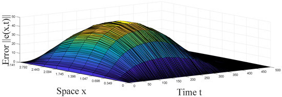
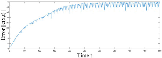
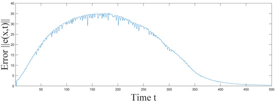
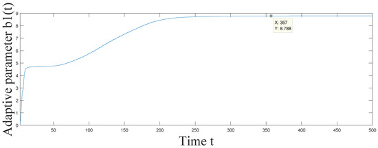
Figure 5.
Trajectory of control parameter of the adaptive controller (36) in Example 1.
5. Conclusions
Pinning and adaptive synchronization of fractional complex networks with impulses and reaction–diffusion terms is investigated in this paper. In order to analyze the stability of the fractional systems with impulsive effects, two special Lyapunov functions with fractional integration terms are constructed and the Lyapunov method is applied. By designing appropriate controllers and adaptive laws, some sufficient criteria for pinning and adaptive synchronization of fractional complex networks with time-varying delays are derived. In addition, a pinning scheme is proposed in which some delay-coupled nodes should be prioritized for pinning. Finally, a numerical example is given to demonstrate the effectiveness and correctness of the main results. A goal of our future investigations is to study more general impulsive fractional systems and analyze the dynamical behaviors of these special systems.
Author Contributions
Writing—original draft preparation, X.H.; writing—review and editing, G.R., Y.Y. and C.X.
Funding
This research is supported by the National Natural Science Foundation of China (No. 61772063) and Beijing Natural Science Foundation (Z180005).
Conflicts of Interest
The authors declare no conflict of interest.
References
- Bernardo, A.H.; Lada, A.A. Internet: Growth dynamics of the World-Wide Web. Nature 1999, 401, 131. [Google Scholar]
- Ding, W.Y.; Wei, X.C.; Yi, D. A closed-form solution for the impedance calculation of grid power distribution network. IEEE Trans. Electromagn. Compat. 2017, 59, 1449–1456. [Google Scholar] [CrossRef]
- Strogatz, S.H. Exploring complex networks. Nature 2001, 410, 268–276. [Google Scholar] [CrossRef]
- Selvaraj, P.; Sakthivel, R.; Kwon, O.M. Synchronization of fractional-order complex dynamical network with random coupling delay, actuator faults and saturation. Nonlinear Dyn. 2018, 94, 3101–3116. [Google Scholar] [CrossRef]
- Yih-Fang, H.; Stefan, W.; Jing, H.; Neelabh, K.; Vijay, G. State estimation in electric power grids: Meeting new challenges presented by the requirements of the future grid. IEEE Signal Process. Mag. 2012, 29, 33–43. [Google Scholar]
- Luo, S.X.; Deng, F.Q.; Chen, W.H. Pointwise-in-space stabilization and synchronization of a class of reaction-diffusion systems with mixed time delays via aperiodically impulsive control. Nonlinear Dyn. 2017, 88, 2899–2914. [Google Scholar] [CrossRef]
- Mo, L.P.; Lin, P. Distributed consensus of second-order multiagent systems with nonconvex input constraints. Int. J. Robust Nonlinear Control. 2018, 28, 3657–3664. [Google Scholar] [CrossRef]
- Mo, L.P.; Guo, S.Y.; Yu, Y.G. Mean-square consensus of heterogeneous multi-agent systems with nonconvex constraints, Markovian switching topologies and delays. Neurocomputing 2018, 291, 167–174. [Google Scholar] [CrossRef]
- Wang, K.H.; Fu, X.C.; Li, K.Z. Cluster synchronization in community networks with nonidentical nodes. Chaos 2009, 19, 023106. [Google Scholar] [CrossRef]
- Liu, S.T.; Zhang, F.F. Complex function projective synchronization of complex chaotic system and its applications in secure communication. Nonlinear Dyn. 2014, 76, 1087–1097. [Google Scholar] [CrossRef]
- Li, C.G.; Chen, G.R. Synchronization in general complex dynamical networks with coupling delays. Physica A 2004, 343, 263–278. [Google Scholar] [CrossRef]
- Wu, X.J.; Lu, H.T. Projective lag synchronization of the general complex dynamical networks with distinct nodes. Commun. Nonlinear Sci. Numer. Simul. 2012, 17, 4417–4429. [Google Scholar] [CrossRef]
- Yu, C.B.; Qin, J.H.; Gao, H.J. Cluster synchronization in directed networks of partial-state coupled linear systems under pinning control. Automatica 2014, 50, 2341–2349. [Google Scholar] [CrossRef]
- Yi, J.W.; Wang, Y.W.; Xiao, J.W.; Huang, Y.H. Exponential synchronization of complex dynamical networks with Markovian jump parameters and stochastic delays and its application to multi-agent systems. Commun. Nonlinear Sci. Numer. Simul. 2013, 18, 1175–1192. [Google Scholar] [CrossRef]
- Selvaraj, P.; Kwon, O.M.; Sakthivel, R. Disturbance and uncertainty rejection performance for fractional-order complex dynamical networks. Neural Netw. 2019, 112, 73–84. [Google Scholar] [CrossRef]
- Chen, J.; Lu, J.A.; Wu, X.Q.; Zheng, W.X. Generalized synchronization of complex dynamical networks via impulsive control. Chaos 2009, 19, 043119. [Google Scholar] [CrossRef]
- Zhang, Q.; Lu, J.A.; Lu, J.H.; Tse, C.K. Adaptive feedback synchronization of a general complex dynamical network with delayed nodes. IEEE Trans. Circuits Syst. II Express Briefs 2008, 55, 183–187. [Google Scholar] [CrossRef]
- Chen, H.W.; Liang, J.L.; Wang, Z.D. Pinning controllability of autonomous Boolean control networks. Sci. China-Inf. Sci. 2016, 59, 070107. [Google Scholar] [CrossRef]
- Liu, X.W.; Chen, T.P. Synchronization of complex networks via aperiodically intermittent pinning control. IEEE Trans. Autom. Control. 2015, 60, 3316–3321. [Google Scholar] [CrossRef]
- Wang, G.S.; Xiao, J.W.; Wang, Y.W.; Yi, J.W. Adaptive pinning cluster synchronization of fractional-order complex dynamical networks. Appl. Math. Comput. 2014, 231, 347–356. [Google Scholar] [CrossRef]
- Chai, Y.; Chen, L.P.; Wu, R.C.; Sun, J. Adaptive pinning synchronization in fractional-order complex dynamical networks. Physica A 2012, 391, 5746–5758. [Google Scholar] [CrossRef]
- Wang, J.L.; Wu, H.N.; Guo, L. Novel adaptive strategies for synchronization of linearly coupled neural networks with reaction-diffusion terms. IEEE Trans. Neural Netw. Learn. Syst. 2014, 25, 429–440. [Google Scholar] [CrossRef]
- Wang, J.L.; Wu, H.N. Passivity of delayed reaction-diffusion networks with application to a food Web model. Appl. Math. Comput. 2013, 219, 11311–11326. [Google Scholar] [CrossRef]
- Wang, J.L.; Wu, H.N.; Huang, T.W.; Ren, S.Y.; Wu, J.G. Pinning controlfor synchronization of coupled reaction-diffusion neural networks with directed topologies. IEEE Trans. Syst. Man Cybern. Syst. 2016, 46, 1109–1120. [Google Scholar] [CrossRef]
- Song, Q.K.; Yan, H.; Zhao, Z.J.; Liu, Y.R. Global exponential stability of complex-valued neural networks with both time-varying delays and impulsive effects. Neural Netw. 2016, 79, 108–116. [Google Scholar] [CrossRef]
- Zhu, Q.X.; Cao, J.D. Stability analysis of Markovian jump stochastic BAM neural networks with impulsive control and mixed time delays. Nature 2012, 13, 2259–2270. [Google Scholar]
- Keith, B.O.; Jerome, S. The Fractional Calculus; Academic Press: New York, NY, USA, 1974. [Google Scholar]
- Ionescu, C.; Lopes, A.; Copot, D.; Machado, J.A.T.; Bates, J.H.T. The role of fractional calculus in modeling biological phenomena: A review. Commun. Nonlinear Sci. Numer. Simul. 2017, 51, 141–159. [Google Scholar] [CrossRef]
- Magin, R.; Ortigueira, M.D.; Podlubny, I.; Trujillo, J. On the fractional signals and systems. Signal Process. 2011, 91, 350–371. [Google Scholar] [CrossRef]
- Park, M.; Lee, S.H.; Kwon, O.M.; Seuret, A. Closeness-Centrality-Based Synchronization Criteria for Complex Dynamical Networks With Interval Time-Varying Coupling Delays. IEEE Trans. Cybern. 2018, 48, 2192–2202. [Google Scholar] [CrossRef]
- Li, X.D.; Zhang, X.L.; Song, S.J. Effect of delayed impulses on input-to-state stability of nonlinear systems. Automatica 2017, 76, 378–382. [Google Scholar] [CrossRef]
- Wang, H.; Yu, Y.G.; Wen, G.G.; Zhang, S.; Yu, J.Z. Global stability analysis of fractional-order Hopfield neural networks with time delay. Neurocomputing 2015, 154, 15–23. [Google Scholar] [CrossRef]
- Kilbas, A.A.; Srivastava, H.M.; Trujillo, J.J. Theory and Applications of Fractional Differential Equations; Elsevier: Amsterdam, The Netherlands, 2006. [Google Scholar]
- Stamova, I. Global Mittag-Leffler stability and synchronization of impulsive fractional-order neural networks with time-varying delays. Nonlinear Dyn. 2014, 77, 1251–1260. [Google Scholar] [CrossRef]
- Lu, J.G. Global exponential stability and periodicity of reaction-diffusion delayed recurrent neural networks with Dirichlet boundary conditions. Chaos 2008, 35, 116–125. [Google Scholar] [CrossRef]
- Boyd, S.; El Ghaoui, L.; Feron, E.; Balakrishnan, V. Linear Matrix Inequalities in System and Control Theory. In Semidefinite Programming and Linear Matrix Inequalities; Society for Industrial and Applied Mathematics: Philadelphia, PA, USA, 1994. [Google Scholar]
- Liu, S.; Li, X.Y.; Zhou, X.F.; Jiang, W. Synchronization analysis of singular dynamical networks with unbounded time-delays. Adv. Differ. Equations 2015, 2015, 193. [Google Scholar] [CrossRef][Green Version]
- Chen, T.P.; Liu, X.W.; Lu, W.L. Pinning complex networks by a single controller. IEEE Trans. Circuits Syst. I Regul. Pap. 2007, 54, 1317–1326. [Google Scholar] [CrossRef]
- Roger, A.H.; Charles, R.J. Topics in Matrix Analysis; Cambridge University Press: Cambridge, UK, 1994. [Google Scholar]
- Roger, A.H.; Charles, R.J. Matrix Analysis; Cambridge University Press: Cambridge, UK, 1985. [Google Scholar]
- Zhang, W.B.; Wang, Z.D.; Liu, Y.R.; Ding, D.R.; Alsaadi, F.E. Event-based state estimation for a class of complex networks with time-varying delays: A comparison principle approach. Phys. Lett. A 2017, 381, 10–18. [Google Scholar] [CrossRef]
- Feng, J.W.; Yang, P.; Zhao, Y. Cluster synchronization for nonlinearly time-varying delayed coupling complex networks with stochastic perturbation via periodically intermittent pinning control. Appl. Math. Comput. 2016, 291, 52–68. [Google Scholar] [CrossRef]
- Lu, R.Q.; Yu, W.W.; Lu, J.H.; Xue, A.K. Synchronization on Complex Networks of Networks. IEEE Trans. Neural Netw. Learn. Syst. 2014, 25, 2110–2118. [Google Scholar] [CrossRef]
- Abbaszadeh, M.; Marquez, H.J. Nonlinear Observer Design for One-Sided Lipschitz Systems. In Proceedings of the 2010 American Control Conference, Baltimore, MD, USA, 30 June–2 July 2010; pp. 5284–5289. [Google Scholar]
- Chen, Y.; Yu, W.W.; Tan, S.L.; Zhu, H.H. Synchronizing nonlinear complex networks via switching disconnected topology. Automatica 2016, 70, 189–194. [Google Scholar] [CrossRef]
- Li, Y.; Chen, Y.Q.; Podlubny, I. Mittag-Leffler stability of fractional order nonlinear dynamic systems. Automatica 2009, 45, 1965–1969. [Google Scholar] [CrossRef]
- Li, Y.; Chen, Y.Q.; Podlubny, I. Stability of fractional-order nonlinear dynamic systems: Lyapunov direct method and generalized Mittag-Leffler stability. Comput. Math. Appl. 2010, 59, 1810–1821. [Google Scholar] [CrossRef]
- Rivero, M.; Rogosin, S.V.; Tenreiro Machado, J.A.; Trujillo, J.J. Stability of Fractional Order Systems. Math. Probl. Eng. 2013, 2013, 356215. [Google Scholar] [CrossRef]
- Sabatier, J.; Farges, C.; Trigeassou, J.C. A stability test for non-commensurate fractional order systems. Syst. Control. Lett. 2013, 62, 739–746. [Google Scholar] [CrossRef]
© 2019 by the authors. Licensee MDPI, Basel, Switzerland. This article is an open access article distributed under the terms and conditions of the Creative Commons Attribution (CC BY) license (http://creativecommons.org/licenses/by/4.0/).