Time-Fractional Diffusion-Wave Equation with Mass Absorption in a Sphere under Harmonic Impact

Abstract

The time-fractional diffusion equation with mass absorption in a sphere is considered under harmonic impact on the surface of a sphere. The Caputo time-fractional derivative is used. The Laplace transform with respect to time and the finite sin-Fourier transform with respect to the spatial coordinate are employed. A graphical representation of the obtained analytical solution for different sets of the parameters including the order of fractional derivative is given.

1. Introduction

The classical parabolic diffusion equation with heat or mass absorption [1]

$$\frac{\partial u}{\partial t}=a\Delta u-bu$$

(1)

also describes bioheat transfer, lateral surface mass or heat exchange in a thin plate, heating of tissue during laser treatment irradiation, etc. (see, for example [2,3,4,5]). The Klein-Gordon equation

$$\frac{{\partial }^{2}u}{\partial t^2}=a\Delta u-bu$$

(2)

is used in solid state physics, classical mechanics, nonlinear optics, and quantum field theory [6,7].

The time-fractional equation

$$\frac{{\partial }^{\alpha }u}{\partial t^{\alpha }}=a\Delta u-bu,0<\alpha \le 2,$$

(3)

can be considered as the extension of the parabolic Equation (1) and hyperbolic Equation (2) and was studied in several publications [8,9,10,11,12,13,14].

It should be noted that such a generalization of many classical differential equations with integer derivatives has numerous applications in rheology, geology, physics, plasma physics, chemistry, geophysics, engineering, biology, bio-engineering, finance, and medicine (see [15,16,17,18,19,20,21,22,23,24,25,26,27,28,29], among many others). There is a great variety of inhomogeneous media where transport phenomena exhibit anomalous properties, the investigation of which is essential to refine understanding the basic characteristics of complex systems widely met in nature. Therefore, studying fractional equations has generated increasing attention of scientists in many disciplines. At present, the fractional diffusion-wave equation is generally used to describe a large class of systems at different scales (from the molecular [30] to the space one [31]) which cover media of the diverse nature (from plasma physics [29] to living tissue [3]). The study of this equation is also of interest from the point of view of understanding the complex spatio-temporal dynamics in nonlinear systems of fractional order [32,33].

In Equation (3) and further in this paper, for more concise notation, $\frac{{\mathrm{d}}^{\alpha }f\left(t\right)}{\mathrm{d}{t}^{\alpha }}$ denotes the Caputo fractional derivative [16,34]

$$\frac{{\mathrm{d}}^{\alpha }f\left(t\right)}{\mathrm{d}{t}^{\alpha }}=\frac{1}{\mathsf{\Gamma }(n-\alpha )}{\int }_0^t{(t-\tau )}^{n-\alpha -1}\frac{{\mathrm{d}}^{n}f\left(\tau \right)}{\mathrm{d}{\tau }^n}\mathrm{d}\tau ,n-1<\alpha <n,$$

(4)

and $\mathsf{\Gamma }\left(\alpha \right)$ denotes the gamma function.

Ångström was the first to investigate the standard parabolic heat conduction equation under harmonic impact and laid the foundations for the new area of study known as “oscillatory diffusion” or “diffusion-waves” (see [35,36,37] and references therein). Periodic solutions of the bioheat equation were investigated in [38]. The harmonic point source in the bioheat equation was used in therapeutic hypotermia [39,40]; applications of the time-harmonic impact in ultrasound surgery were studied in [41].

As a rule, in the previous studies of diffusion or heat conduction equation the quasi-steady-state oscillations were investigated when the solution $u(\mathbf{x},t)$ was represented as a product of a function of the spatial coordinates $U\left(\mathbf{x}\right)$ and the time-harmonic term ${\mathrm{e}}^{i\omega t}$ with the angular frequency $\omega$

$$u(\mathbf{x},t)=U\left(\mathbf{x}\right){\mathrm{e}}^{i\omega t}$$

(5)

without consideration of the initial conditions.

The use of assumption (5) is based on the well known formula for the derivative of the integer order n of the exponential function

$$\frac{{\mathrm{d}}^n{\mathrm{e}}^{\lambda t}}{\mathrm{d}{t}^n}={\lambda }^n{\mathrm{e}}^{\lambda t}.$$

(6)

In the event of the non-integer order of time derivative, the assumption (5) cannot be used since [42]

$$\frac{{\mathrm{d}}^{\alpha }{\mathrm{e}}^{\lambda t}}{\mathrm{d}{t}^{\alpha }}={\lambda }^{\alpha }{\mathrm{e}}^{\lambda t}\frac{\gamma (n-\alpha ),\lambda t)}{\mathsf{\Gamma }(n-\alpha )}\ne {\lambda }^{\alpha }{\mathrm{e}}^{\lambda t},n-1<\alpha <n,$$

(7)

with $\gamma (a,x)$ being the incomplete gamma function [43]

$$\gamma (a,x)={\int }_0^x{\mathrm{e}}^{-u}{u}^{a-1}\mathrm{d}u.$$

(8)

It is worthy of notice that for the Riemann-Liouville fractional derivative [16,34] with the lower limit of integration at 0

$$D_{RL}^{\alpha }f\left(t\right)=\frac{{\mathrm{d}}^n}{\mathrm{d}{t}^n}\left[\frac{1}{\mathsf{\Gamma }(n-\alpha )}{\int }_0^t{(t-\tau )}^{n-\alpha -1}f\left(\tau \right)\mathrm{d}\tau \right],n-1<\alpha <n,$$

(9)

we also have [16]

$$D_{RL}^{\alpha }{\mathrm{e}}^{\lambda t}=t^{-\alpha }{E}_{1,1-\alpha }\left(\lambda t\right)\ne {\lambda }^{\alpha }{\mathrm{e}}^{\lambda t}.$$

(10)

Here $E_{\alpha ,\beta }\left(z\right)$ is the Mittag-Leffler function in two parameters $\alpha$ and $\beta$ [16,34]

$$E_{\alpha ,\beta }\left(z\right)={\displaystyle \sum _{n=0}^{\infty }}\frac{z^n}{\mathsf{\Gamma }(\alpha n+\beta )},\Re \left(\alpha \right)>0,\beta \in C,z\in C.$$

(11)

In this paper, the initial-boundary-value problem for Equation (3) is studied in a spherical domain for the case of central symmetry under the Dirichlet boundary condition varying harmonically in time. The present paper develops and extends the results of the previous investigations [44,45], where the corresponding problems for line and half-line domains were investigated.

2. Statement of the Problem

The time-fractional diffusion equation with mass absorption (mass release) is examined in a sphere

$$\frac{{\partial }^{\alpha }u}{\partial t^{\alpha }}=a\left(\frac{{\partial }^{2}u}{\partial r^2}+\frac{2}{r}\frac{\partial u}{\partial r}\right)-bu,0<r<R,0<t<\infty ,0<\alpha \le 2,$$

(12)

under zero initial conditions

$$\begin{array}{cc}\hfill t=0:& u=0,0<\alpha \le 2,\hfill \end{array}$$

(13)

$$\begin{array}{cc}\hfill t=0:& \frac{\partial u}{\partial t}=0,1<\alpha \le 2,\hfill \end{array}$$

(14)

and harmonic impact on the surface of a sphere

$$r=R:u=u_0{\mathrm{e}}^{i\omega t}.$$

(15)

As in the case of classical diffusion equation (when $\alpha =1$) and the wave equation (when $\alpha =2$) the boundedness condition at the origin is also adopted:

$$r=0:u\ne \infty .$$

(16)

In what follows, the integral transform technique will be used. Recall the Laplace transform rule for the Caputo derivative

$$\mathcal{L}\left\{\frac{{\mathrm{d}}^{\alpha }f\left(t\right)}{\mathrm{d}{t}^{\alpha }}\right\}=s^{\alpha }{f}^{*}\left(s\right)-{\displaystyle \sum _{k=0}^{n-1}}{f}^{\left(k\right)}\left(0^{+}\right)s^{\alpha -1-k},n-1<\alpha <n,$$

(17)

where the transform is marked by the asterisk, and s is the Laplace transform variable.

The following finite sin-Fourier transform is amenable to the central symmetric problem in a spherical domain $0\le r\le R$ [46]. For the Dirichlet boundary condition:

$$\mathcal{F}\left\{f\left(r\right)\right\}=\tilde{f}\left({\xi }_k\right)={\int }_0^{R}rf\left(r\right)\frac{sin\left(r{\xi }_k\right)}{{\xi }_k}\mathrm{d}r,$$

(18)

$${\mathcal{F}}^{-1}\left\{\tilde{f}\left({\xi }_k\right)\right\}=f\left(r\right)=\frac{2}{R}{\displaystyle \sum _{k=1}^{\infty }}{\xi }_k\tilde{f}\left({\xi }_k\right)\frac{sin\left(r{\xi }_k\right)}{r},$$

(19)

where the transform is marked by the tilde, and

$${\xi }_k=\frac{k\pi }{R}$$

(20)

is the Fourier transform variable.

For the central symmetric Laplace operator

$$\mathcal{F}\left\{\frac{{\mathrm{d}}^{2}f\left(r\right)}{\mathrm{d}{r}^2}+\frac{2}{r}\frac{\mathrm{d}f\left(r\right)}{\mathrm{d}r}\right\}=-{\xi }_k^2\tilde{f}\left({\xi }_k\right)+{(-1)}^{k+1}Rf\left(R\right).$$

(21)

Applying to the problems (12)–(16) the Laplace transform with respect to time t and the finite sin-Fourier transform (18) with respect to the radial coordinate r, we get in the transform domain

$${\tilde{u}}^{*}({\xi }_k,s)={(-1)}^{k+1}aR{u}_0\frac{1}{s^{\alpha }+a{\xi }_k^2+b}\frac{1}{s-i\omega }.$$

(22)

The solution is obtained after inversion of the integral transforms:

$$u(r,t)=\frac{2a{u}_0}{r}{\displaystyle \sum _{k=1}^{\infty }}{(-1)}^{k+1}{\xi }_{k}sin\left(r{\xi }_k\right){\int }_0^t{\tau }^{\alpha -1}{E}_{\alpha ,\alpha }\left[-\left(a{\xi }_k^2+b\right){\tau }^{\alpha }\right]{\mathrm{e}}^{i\omega (t-\tau )}\mathrm{d}\tau ,$$

(23)

where $E_{\alpha ,\beta }\left(z\right)$ is the Mittag-Leffler function (11), and the convolution theorem as well as the following equation for the inverse Laplace transform [16]

$${\mathcal{L}}^{-1}\left\{\frac{s^{\alpha -\beta }}{s^{\alpha }+\gamma }\right\}=t^{\beta -1}{E}_{\alpha ,\beta }\left(-\gamma t^{\alpha }\right),\alpha >0,\beta >0,$$

(24)

have been used.

In numerical calculations, the nondimensional quantities are used:

$$\begin{array}{c}\overline{u}=\frac{u}{u_0},\overline{r}=\frac{r}{R},\overline{t}=\frac{a^{1/\alpha }}{R^{2/\alpha }}t,\overline{\omega }=\frac{R^{2/\alpha }}{a^{1/\alpha }}\omega ,\\ \overline{b}=\frac{R^2}{a}b,{\eta }_k=R{\xi }_k=k\pi .\end{array}$$

(25)

Hence, using in integral in (23) the substitution $\tau =tw$, for the real part of the solution we get

$$\overline{u}(\overline{r},\overline{t},\overline{b},\overline{\omega })=\frac{2{\overline{t}}^{\alpha }}{\overline{r}}{\displaystyle \sum _{k=1}^{\infty }}{(-1)}^{k+1}{\eta }_{k}sin\left(\overline{r}{\eta }_k\right){\int }_0^1{w}^{\alpha -1}{E}_{\alpha ,\alpha }\left[-\left({\eta }_k^2+\overline{b}\right){\overline{t}}^{\alpha }{w}^{\alpha }\right]cos\left[\overline{\omega }\overline{t}(1-w)\right]\mathrm{d}w,$$

(26)

where we can see that the solution $\overline{u}$ depends not only on time and spatial coordinate, but also on the parameters $\overline{b}$ and $\overline{\omega }$.

To simplify calculations, it would be worthwhile to introduce a substitution $z=w^{\alpha }.$ Hence,

$$\overline{u}(\overline{r},\overline{t},\overline{b},\overline{\omega })=\frac{2{\overline{t}}^{\alpha }}{\overline{r}}{\displaystyle \sum _{k=1}^{\infty }}{(-1)}^{k+1}{\eta }_{k}sin\left(\overline{r}{\eta }_k\right){\int }_0^1{E}_{\alpha ,\alpha }\left[-\left({\eta }_k^2+\overline{b}\right){\overline{t}}^{\alpha }z\right]cos\left[\overline{\omega }\overline{t}\left(1-z^{1/\alpha }\right)\right]\mathrm{d}z.$$

(27)

To evaluate the Mittag-Leffler function the algorithms suggested in [47] were used; see also the MATLAB function [48] that implements these algorithms.

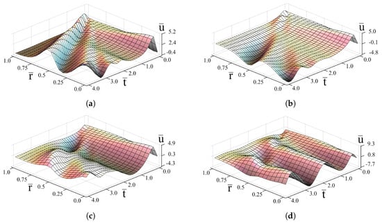
The numerical results are shown in Figure 1, Figure 2, Figure 3, Figure 4 and Figure 5. Calculations were carried out for the grid size step $\Delta \overline{t}=0.1$, $\Delta \overline{r}=0.05$. A graphical representation of the solution (27) makes it possible to analyze not only the limiting cases of the problem (see Section 3), but also to understand the influence of the main parameters of the problem (including the value of the order of fractional derivative) on the spatial-temporal evolution of the solution.

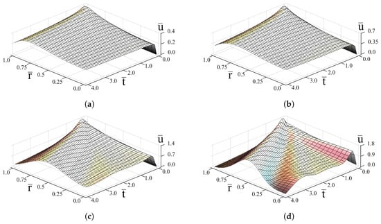
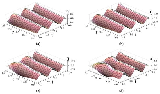
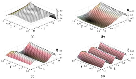
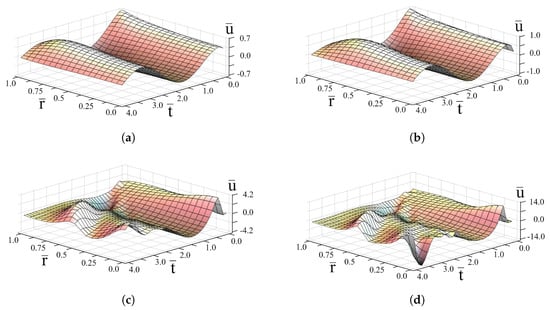
It is seen from Figures that time oscillations of the solution are governed by the harmonic term ${\mathrm{e}}^{i\omega t}$. The increasing of absorption parameter b decreases the oscillation amplitude (Figure 2b and Figure 3d), whereas increasing $\alpha$ increases it (Figure 2a–d and Figure 3d). As the Mittag-Leffler function

$$E_{2,2}\left(-x^2\right)=\frac{sinx}{x},$$

(28)

the space oscillations of the solution depending on the order of fractional derivative appear for $\alpha \ge 1.5$ (Figure 1d and Figure 2d) and become well-marked for $\alpha$ approaching 2. The influence of both factors is evident from Figure 4 and Figure 5.

3. Analysis of the Quasi-Steady-State Oscillations

Now, we shall investigate two particular cases of the problem studied in the previous section corresponding to the integer values of the order of time derivative. For $\alpha =1$, we have

$${\tilde{u}}^{*}({\xi }_k,s)={(-1)}^{k+1}aR{u}_0\frac{1}{s+a{\xi }_k^2+b}\frac{1}{s-i\omega }.$$

(29)

Taking into account that [49]

$${\mathcal{L}}^{-1}\left\{\frac{1}{\left(s+p\right)\left(s+q\right)}\right\}=\frac{{\mathrm{e}}^{-qt}-{\mathrm{e}}^{-pt}}{p-q},$$

(30)

we arrive at the solution to the bioheat equation

$$\begin{array}{ll}u(r,t)& =\frac{2a{u}_0}{r}{\displaystyle \sum _{k=1}^{\infty }}{\left(-1\right)}^{k+1}\frac{{\xi }_{k}sin\left(r{\xi }_k\right)}{a{\xi }_k^2+b+i\omega }{\mathrm{e}}^{i\omega t}\\ & -\frac{2a{u}_0}{r}{\displaystyle \sum _{k=1}^{\infty }}{\left(-1\right)}^{k+1}\frac{{\xi }_{k}sin\left(r{\xi }_k\right)}{a{\xi }_k^2+b+i\omega }{\mathrm{e}}^{-\left(a{\xi }_k^2+b\right)t}.\end{array}$$

(31)

Similarly, for $\alpha =2$,

$${\tilde{u}}^{*}({\xi }_k,s)={(-1)}^{k+1}aR{u}_0\frac{1}{s^2+a{\xi }_k^2+b}\frac{1}{s-i\omega }.$$

(32)

Taking into consideration that [49]

$${\mathcal{L}}^{-1}\left\{\frac{1}{\left(s^2+p^2\right)\left(s+q\right)}\right\}=\frac{1}{p^2+q^2}\left[{\mathrm{e}}^{-qt}-cos\left(pt\right)+\frac{q}{p}sin\left(pt\right)\right],$$

(33)

we obtain the solution to the Klein-Gordon equation

$$\begin{array}{ll}u(r,t)& =\frac{2a{u}_0}{r}{\displaystyle \sum _{k=1}^{\infty }}{\left(-1\right)}^{k+1}\frac{{\xi }_{k}sin\left(r{\xi }_k\right)}{a{\xi }_k^2+b-{\omega }^2}{\mathrm{e}}^{i\omega t}\\ & -\frac{2a{u}_0}{r}{\displaystyle \sum _{k=1}^{\infty }}{\left(-1\right)}^{k+1}\frac{{\xi }_{k}sin\left(r{\xi }_k\right)}{a{\xi }_k^2+b-{\omega }^2}\left[cos\left(\sqrt{a{\xi }_k^2+b}t\right)+\frac{i\omega }{\sqrt{a{\xi }_k^2+b}}sin\left(\sqrt{a{\xi }_k^2+b}t\right)\right].\end{array}$$

(34)

For integer $\alpha$, we can assume that

$$u(r,t)=U\left(r\right){\mathrm{e}}^{i\omega t}.$$

(35)

For $\alpha =1$, the function $U\left(r\right)$ fulfills the equation

$$\frac{{\mathrm{d}}^{2}U}{\mathrm{d}{r}^2}+\frac{2}{r}\frac{\mathrm{d}U}{\mathrm{d}r}-\frac{b+i\omega }{a}U=0,$$

(36)

under the boundary condition

$$r=R:U\left(r\right)=u_0,$$

(37)

and for $b>0$ has the solution bounded at the origin

$$U\left(r\right)=\frac{R{u}_0}{r}\frac{sinh\left[r\sqrt{(b+i\omega )/a}\right]}{sinh\left[R\sqrt{(b+i\omega )/a}\right]}.$$

(38)

Therefore,

$$u(r,t)=\frac{R{u}_0}{r}\frac{sinh\left[r\sqrt{(b+i\omega )/a}\right]}{sinh\left[R\sqrt{(b+i\omega )/a}\right]}{\mathrm{e}}^{i\omega t}$$

(39)

(for negative value of b, sinh will be substituted by sin).

The first term in the solution (31) can be evaluated analytically using the following formula [50]

$${\displaystyle \sum _{k=1}^{\infty }}{\left(-1\right)}^{k+1}\frac{k}{k^2+p^2}sin\left(kr\right)=\frac{\pi }{2}\frac{sinh\left(rp\right)}{sinh\left(\pi p\right)},-\pi <r<\pi ,.$$

(40)

$${\displaystyle \sum _{k=1}^{\infty }}{\left(-1\right)}^{k+1}\frac{k}{k^2-p^2}sin\left(kr\right)=\frac{\pi }{2}\frac{sin\left(rp\right)}{sin\left(\pi p\right)},-\pi <r<\pi .$$

(41)

It was emphasized in [51] that Equation (41) is also valid for complex values of p and hence turns into Equation (40) for imaginary p.

Taking into account Equation (40), we obtain that the first term in the solution (31) coincides with the quasi-steady-state solution (39), whereas the second term in Equation (31) describes the transient process.

The similar analysis can be carried out for $\alpha =2$ based on the assumption (35). In this case, the function $U\left(r\right)$ fulfills the equation

$$\frac{{\mathrm{d}}^{2}U}{\mathrm{d}{r}^2}+\frac{2}{r}\frac{\mathrm{d}U}{\mathrm{d}r}-\frac{b-{\omega }^2}{a}U=0,$$

(42)

under the boundary condition

$$r=R:U\left(r\right)=u_0,$$

(43)

and for $b>{\omega }^2$ has the solution bounded at the origin

$$U\left(r\right)=\frac{R{u}_0}{r}\frac{sinh\left[r\sqrt{(b-{\omega }^2)/a}\right]}{sinh\left[R\sqrt{(b-{\omega }^2)/a}\right]},$$

(44)

whereas for $b<{\omega }^2$

$$U\left(r\right)=\frac{R{u}_0}{r}\frac{sin\left[r\sqrt{({\omega }^2-b)/a}\right]}{sin\left[R\sqrt{({\omega }^2-b)/a}\right]}.$$

(45)

Hence, for $b>{\omega }^2$

$$u(r,t)=\frac{R{u}_0}{r}\frac{sinh\left[r\sqrt{(b-{\omega }^2)/a}\right]}{sinh\left[R\sqrt{(b-{\omega }^2)/a}\right]}{\mathrm{e}}^{i\omega t}.$$

(46)

and for $b<{\omega }^2$

$$u(r,t)=\frac{R{u}_0}{r}\frac{sin\left[r\sqrt{({\omega }^2-b)/a}\right]}{sin\left[R\sqrt{({\omega }^2-b)/a}\right]}{\mathrm{e}}^{i\omega t}.$$

(47)

The first term in the solution (34) after accounting for Equations (40) and (41) coincides with the quasi-steady-state solutions (46) and (47), respectively, whereas the second term in (34) describes the transient process.

4. Conclusions

The time-fractional diffusion-wave equation with the Caputo fractional derivative of the order $0<\alpha \le 2$ with mass absorption was studied in a spherical domain under the Dirichlet boundary condition varying harmonically in time. The Caputo derivative of the exponential function has a much more complicated form than the corresponding derivative of the integer order. Hence, the assumption that the solution of the problem can be represented as a product of a function of the spatial coordinate and the time-harmonic term without consideration of the initial conditions cannot be used. The solution is obtained using the Laplace transform with respect to time and the finite sin-Fourier transform specifically adapted for a spherical domain and is expressed in terms of the Mittag-Leffler function. A graphical representation of the obtained analytical solution demonstrates the influence of the main parameters of the problem including the value of the order of fractional derivative on the spatial-temporal evolution of the solution.

References

- Crank, J. The Mathematics of Diffusion, 2nd ed.; Clarendon Press: Oxford, UK, 1975. [Google Scholar]
- Pennes, H.H. Analysis of tissue and arterial blood temperatures in the resting human forearm. J. Appl. Physiol. 1948, 1, 93–122. [Google Scholar] [CrossRef] [PubMed]
- Gafiychuk, V.V.; Lubashevsky, I.A.; Datsko, B.Y. Fast heat propagation in living tissue caused by branching artery network. Phys. Rev. E 2005, 72, 051920. [Google Scholar] [CrossRef]
- Datsko, B.Y.; Gafiychuk, V.V.; Lubashevsky, I.A.; Priezzhev, A.V. Self-localization of laser-induced tumor coagulation limited by heat diffusion through active tissue. J. Med. Eng. Technol. 2006, 30, 390–396. [Google Scholar] [CrossRef]
- Polyanin, A.D. Handbook of Linear Partial Differential Equations for Engineers and Scientists; Chapman & Hall/CRC: Boca Raton, FL, USA, 2002. [Google Scholar]
- Gravel, P.; Gauthier, C. Classical applications of the Klein-Gordon equation. Am. J. Phys. 2011, 79, 447–453. [Google Scholar] [CrossRef]
- Wazwaz, A.-M. Partial Differential Equations and Solitary Waves Theory; Higher Education Press: Beijing, China; Springer: Berlin, Germany, 2009. [Google Scholar]
- Abuteen, A.; Freihat, A.; Al-Smadi, M.; Khalil, H.; Khan, R.A. Approximate series solution of nonlinear, fractional Klein-Gordon equations using fractional reduced differential transform method. J. Math. Stat. 2016, 12, 23–33. [Google Scholar] [CrossRef]
- Damor, R.S.; Kumar, S.; Shukla, A.K. Solution of fractional bioheat equation in terms of Fox’s H-Function. SpringerPlus 2016, 5, 1–10. [Google Scholar] [CrossRef]
- Ferrás, L.L.; Ford, N.J.; Morgado, M.L.; Nóbrega, J.M.; Rebelo, M.S. Fractional Pennes’ bioheat equation: theoretical and numerical studies. Fract. Calc. Appl. Anal. 2015, 18, 1080–1106. [Google Scholar] [CrossRef]
- Golmankhaneh, A.K.; Golmankhaneh, A.K.; Baleanu, D. On nolinear fractional Klein-Gordon equation. Signal Process. 2011, 91, 446–451. [Google Scholar] [CrossRef]
- Kheiri, H.; Shahi, S.; Mojaver, A. Analytical solutions for the fractional Klein-Gordon equation. Comput. Meth. Diff. Equ. 2014, 2, 99–114. [Google Scholar]
- Qin, Y.; Wu, K. Numerical solution of fractional bioheat equation by quadratic spline collocation method. J. Nonlinear Sci. Appl. 2016, 9, 5061–5072. [Google Scholar] [CrossRef]
- Vitali, S.; Castellani, G.; Mainardi, F. Time fractional cable equation and applications in neurophysiology. Chaos Solitons Fractals 2017, 102, 467–472. [Google Scholar] [CrossRef]
- Gorenflo, R.; Mainardi, F. Fractional calculus: Integral and differential equations of fractional order. In Fractals and Fractional Calculus in Continuum Mechanics; Springer: Wien, Austria, 1997; pp. 223–276. [Google Scholar]
- Podlubny, I. Fractional Differential Equations; Academic Press: San Diego, CA, USA, 1999. [Google Scholar]
- Povstenko, Y. Fractional heat conduction equation and associated thermal stresses. J. Therm. Stress. 2005, 28, 83–102. [Google Scholar] [CrossRef]
- Magin, R.L. Fractional Calculus in Bioengineering; Begell House Publishers, Inc.: Redding, CA, USA, 2006. [Google Scholar]
- Gafiychuk, V.V.; Datsko, B.Y. Spatiotemporal pattern formation in fractional reaction-diffusion systems with indices of different order. Phys. Rev. E 2008, 77, 066210. [Google Scholar] [CrossRef]
- Mainardi, F. Fractional Calculus and Waves in Linear Viscoelasticity: An Introduction to Mathematical Models; Imperial College Press: London, UK, 2010. [Google Scholar]
- Tarasov, V.E. Fractional Dynamics: Applications of Fractional Calculus to Dynamics of Particles, Fields and Media; Springer: Berlin/Heidelberg, Germany, 2010. [Google Scholar]
- Datsko, B.; Luchko, Y.; Gafiychuk, V. Pattern formation in fractional reaction-diffusion systems with multiple homogeneous states. Int. J. Bifurcat. Chaos 2012, 22, 1250087. [Google Scholar] [CrossRef]
- Datsko, B.; Gafiychuk, V. Complex nonlinear dynamics in subdiffusive activator-inhibitor systems. Commun. Nonlinear Sci. Numer. Simul. 2012, 17, 1673–1680. [Google Scholar] [CrossRef]
- Uchaikin, V.V. Fractional Derivatives for Physicists and Engineers; Springer: Berlin, Germany, 2013. [Google Scholar]
- Atanacković, T.M.; Pilipović, S.; Stanković, B.; Zorica, D. Fractional Calculus with Applications in Mechanics: Vibrations and Diffusion Processes; John Wiley & Sons: Hoboken, NJ, USA, 2014. [Google Scholar]
- Herrmann, R. Fractional Calculus: An Introduction for Physicists, 2nd ed.; World Scientific: Singapore, 2014. [Google Scholar]
- Povstenko, Y. Fractional Thermoelasticity; Springer: New York, NY, USA, 2015. [Google Scholar]
- Datsko, B.; Gafiychuk, V.; Podlubny, I. Solitary travelling auto-waves in fractional reaction–diffusion systems. Commun. Nonlinear Sci. Numer. Simul. 2015, 23, 378–387. [Google Scholar] [CrossRef]
- Anderson, J.; Moradi, S.; Rafiq, T. Non-linear Langevin and fractional Fokker-Planck equations for anomalous diffusion by Lévy stable processes. Entropy 2018, 20, 760. [Google Scholar] [CrossRef]
- Weiss, M.; Nilsson, T. In a mirror dimly: Tracing the movements of molecules in living cells. Trends Cell Biol. 2004, 14, 267–273. [Google Scholar] [CrossRef]
- Zelenyi, L.M.; Milovanov, A.V. Fractal topology and strange kinetics: From percolation theory to problems in cosmic electrodynamics. Phys. Uspekhi 2004, 47, 809–852. [Google Scholar] [CrossRef]
- Gafiychuk, V.; Datsko, B. Different types of instabilities and complex dynamics in reaction-diffusion systems with fractional derivatives. J. Comp. Nonlinear Dyn. 2012, 7, 031001. [Google Scholar] [CrossRef]
- Datsko, B.; Gafiychuk, V. Complex spatio-temporal solutions in fractional reaction-diffusion systems near a bifurcation point. Fract. Calc. Appl. Anal. 2018, 21, 237–253. [Google Scholar] [CrossRef]
- Kilbas, A.A.; Srivastava, H.M.; Trujillo, J.J. Theory and Applications of Fractional Differential Equations; Elsevier: Amsterdam, The Netherlands, 2006. [Google Scholar]
- Mandelis, A. Diffusion waves and their uses. Phys. Today 2000, 53, 29–33. [Google Scholar] [CrossRef]
- Mandelis, A. Diffusion-Wave Fields: Mathematical Methods and Green Functions; Springer: New York, NY, USA, 2001. [Google Scholar]
- Vrentas, J.S.; Vrentas, C.M. Diffusion and Mass Transfer; CRC Press: Boca Raton, FL, USA, 2013. [Google Scholar]
- Lakhssassi, A.; Kengne, E.; Semmaoui, H. Modifed Pennes’ equation modelling bio-heat transfer in living tissues: analytical and numerical analysis. Natl. Sci. 2010, 2, 1375–1385. [Google Scholar] [CrossRef]
- Kengne, E.; Lakhssassi, A.; Vaillancourt, R. Temperature distributions for regional hypothermia based on nonlinear bioheat equation of Pennes type: Dermis and subcutaneous tissues. Appl. Math. 2012, 3, 217–224. [Google Scholar] [CrossRef]
- Fasano, A.; Sequeira, A. Hemomath. The Mathematics of Blood; Springer: Cham, Switzerland, 2017. [Google Scholar]
- Malinen, M.; Huttunen, T.; Kaipio, J.P. Thermal dose optimization method for ultrasound surgery. Phys. Med. Biol. 2003, 48, 745–762. [Google Scholar] [CrossRef]
- Povstenko, Y. Fractional heat conduction in a space with a source varying harmonically in time and associated thermal stresses. J. Therm. Stress. 2016, 39, 1442–1450. [Google Scholar] [CrossRef]
- Abramowitz, M.; Stegun, I.A. (Eds.) Handbook of Mathematical Functions with Formulas, Graphs and Mathematical Tables; Dover: New York, NY, USA, 1972. [Google Scholar]
- Povstenko, Y.; Kyrylych, T. Time-fractional diffusion with mass absorption under harmonic impact. Fract. Calc. Appl. Anal. 2018, 21, 118–133. [Google Scholar] [CrossRef]
- Povstenko, Y.; Kyrylych, T. Time-fractional diffusion with mass absorption in a half-line domain due to boundary value of concentration varying harmonically in time. Entropy 2018, 19, 346. [Google Scholar] [CrossRef]
- Povstenko, Y. Linear Fractional Diffusion-Wave Equation for Scientists and Engineers; Birkhäuser: New York, NY, USA, 2015. [Google Scholar]
- Gorenflo, R.; Loutchko, J.; Luchko, Y. Computation of the Mittag-Leffler function and its derivatives. Fract. Calc. Appl. Anal. 2002, 5, 491–518. [Google Scholar]
- Podlubny, I. Mittag-Leffler Function; Calculates the Mittag-Leffler Function with Desired Accuracy, MATLAB Central File Exchange, File ID 8738. Available online: www.mathworks.com/matlabcentral/fileexchange/8738 (accessed on 17 April 2019).
- Erdélyi, A.; Magnus, W.; Oberhettinger, F.; Tricomi, F. Tables of Integral Transforms; McGraw-Hill: New York, NY, USA, 1954; Volume 1. [Google Scholar]
- Prudnikov, A.P.; Brychkov, Y.A.; Marichev, O.I. Integrals and Series, Volume 1: Elementary Functions; Gordon and Breach Science Publishers: Amsterdam, The Netherlands, 1986. [Google Scholar]
- Magnus, W.; Oberhettinger, F. Formeln und Sätze für die Speziellen Funkttionen der Mathematischen Physik, 2nd ed.; Springer: Berlin, Germany, 1948. [Google Scholar]
© 2019 by the authors. Licensee MDPI, Basel, Switzerland. This article is an open access article distributed under the terms and conditions of the Creative Commons Attribution (CC BY) license (http://creativecommons.org/licenses/by/4.0/).