Further Results on the Resistance-Harary Index of Unicyclic Graphs

Abstract

The Resistance-Harary index of a connected graph G is defined as $RH\left(G\right)={\displaystyle \sum _{\{u,v\}\subseteq V\left(G\right)}}\frac{1}{r(u,v)}$, where $r(u,v)$ is the resistance distance between vertices u and v in G. A graph G is called a unicyclic graph if it contains exactly one cycle and a fully loaded unicyclic graph is a unicyclic graph that no vertex with degree less than three in its unique cycle. Let $\mathcal{U}\left(n\right)$ and $\mathfrak{U}\left(n\right)$ be the set of unicyclic graphs and fully loaded unicyclic graphs of order n, respectively. In this paper, we determine the graphs of $\mathcal{U}\left(n\right)$ with second-largest Resistance-Harary index and determine the graphs of $\mathfrak{U}\left(n\right)$ with largest Resistance-Harary index.

1. Introduction

The topological index is the mathematical descriptor of the molecular structure, which can effectively reflect the chemical structure and properties of the material. The famous Wiener index $W\left(G\right)$ (also Wiener number) introduced by H. Wiener, is a topological index of a molecule, defined as the sum of the lengths of the shortest paths between all pairs of vertices, i.e., $W\left(G\right)={\displaystyle \sum _{\{u,v\}\subseteq V\left(G\right)}}d(u,v)$ in the chemical graph representing the non-hydrogen atoms in the molecule.In 1993, Klein and Randić [1] defined a new distance function named resistance distance on the basis of electrical network theory replacing each edge of a simple connected graph G by a unit resistor. Let G be a simple connected graph with vertices set $V=\{v_1,v_2,\cdots ,v_n\}$. The resistance distance between the vertices $v_i$ and $v_j$, denoted by $r(v_i,v_j)$ (if more than one graphs are considered, we write $r_G(v_i,v_j)$ to avoid confusion), is defined to be the effective resistance between the vertices $v_i$ and $v_j$ in G. If the ordinary distance is replaced by resistance distance in the expression for the Wiener index, one arrives at the Kirchhoff index [1,2]

$$Kf\left(G\right)=\sum _{\{u,v\}\subseteq V\left(G\right)}r(u,v),$$

which has been widely studied [3,4,5,6,7,8,9,10,11,12].

Another distance-based graph invariant index named Harary index was introduced independently by Plavšić et al. [13] and by Ivanciuc et al. [14] in 1993 for the characterization of molecular graphs. The Harary index $H\left(G\right)$ is defined as

$$H\left(G\right)=\sum _{\{u,v\}\subseteq V\left(G\right)}\frac{1}{d(u,v)},$$

which is the sum of reciprocals of distances between all pairs of vertices of G. For more related results to Harary index, please refer to [15,16,17,18,19,20,21,22]. In 2017, Chen et al. [23,24] introduced a new graph invariant reciprocal to Kirchhoff index, named Resistance-Harary index, as

$$RH\left(G\right)=\sum _{\{u,v\}\subseteq V\left(G\right)}\frac{1}{r(u,v)}.$$

To understand the results and concepts, we introduce some definitions and notions. All of the graphs considered in this paper are connected and simple. A graph G is called a unicyclic graph if it contains exactly one cycle, simply denoted as $G=U(C_l;T_1,T_2,\cdots ,T_l)$, where $C_l$ is the unique cycle with vertices $v_1{v}_2\cdots v_l$, $T_i$ is a tree rooted at $v_i$, $1\le i\le l$. A fully loaded unicyclic graph is a unicyclic graph with the property that there is no vertex with degree less than three in its unique cycle. Let $S_n^l$ denote the graph obtained from cycle $C_l$ by adding $n-l$ pendant edges to a vertex of $C_l$. Let $\mathcal{U}(n;l)$ be the set of unicyclic graphs with n vertices and the unique cycle $C_l$ and $\mathcal{U}\left(n\right)$ be the set of unicyclic graphs with n vertices. Let $\mathfrak{U}(n;l)$ be the set of all fully loaded unicyclic graphs with n vertices and the unique cycle $C_l$, and $\mathfrak{U}\left(n\right)$ be the set of unicyclic graphs with n vertices. Let $S_n$ and $P_n$ be the star and the path on n vertices, respectively.

In this paper, we improve the results of the recent paper (Chen et al. [23]) and we determine the largest Resistance-Harary index among all unicyclic graphs. Additionally, we determine the second-largest Resistance-Harary index among all unicyclic graphs and determine the largest Resistance-Harary index among all fully loaded unicyclic graphs and characterize the corresponding extremal graphs, respectively.

2. Preliminaries

In this section, we introduce some useful lemmas and two transformations. Let $R_G\left(u\right)={\displaystyle \sum _{u\in V\left(G\right)\setminus \left\{u\right\}}}\frac{1}{r_G(u,v)}$, then $RH\left(G\right)=\frac{1}{2}{\displaystyle \sum _{u\in V\left(G\right)}}{R}_G\left(u\right)$. Let $C_g=v_1{v}_2\cdots v_g{v}_1$ be the cycle on g vertices where $g\ge 3$. By Ohm’s law, for any two vertices $v_i,v_j\in V\left(C_g\right)$ with $i<j$, one has

$$r_{C_g}(v_i,v_j)=\frac{(j-i)(g+i-j)}{g}.$$

By a simple calculation, we can obtain the Resistance-Harary index of $C_g$, which is

$$RH\left(C_g\right)=\sum _{u\in V\left(C_g\right)}\frac{1}{2}{R}_{C_g}\left(v\right)=g\sum _{i=1}^{g-1}\frac{1}{i}$$

Lemma 1 

([1]). Let x be a cut vertex of a connected graph G and let a and b be vertices occurring in different components which arise upon deletion of x. Then,

$$r_G(a,b)=r_G(a,x)+r_G(x,b).$$

Definition 1 

([23]). Let v be a vertex of degree $p+1$ in a graph G, such that $v{v}_1,v{v}_2,\dots ,v{v}_p$ are pendent edges incident with v, and u is the neighbor of v distinct from $v_1,v_2,\dots ,v_p$. We form a graph $G^{\prime }=\sigma (G,v)$ by deleting the edges $v{v}_1,v{v}_2,\dots ,v{v}_p$ and adding new edges $u{v}_1,u{v}_2,\dots ,u{v}_p$. We say that $G^{\prime }$ is a σ-transform of the graph G (see Figure 1).

Lemma 2 

([23]). Let $G^{\prime }=\sigma (G,v)$ be a σ-transform from the graph G, $d\left(u\right)\ge 1$ described in Figure 1. Then, $RH\left(G^{\prime }\right)\ge RH\left(G\right)$, with equality holds if and only if G is a star with v as its center.

Definition 2 

([23]). Let $u,v$ be two vertices in a graph G, such that $u_1,u_2,\cdots ,u_s$ are pendents incident with u and $v_1,v_2,\cdots ,v_t$ are pendents incident with v in $G_0\subseteq G$, respectively. $G^{\prime }$ and $G″$ are two graphs β transformed from G, such that $G^{\prime }=G-\{v{v}_1,v{v}_2,\cdots ,v{v}_t\}+\{u{v}_1,u{v}_2,\cdots ,u{v}_t\}$, $G″=G-\{v{v}_1,v{v}_2,\cdots ,v{v}_s\}+\{u{v}_1,u{v}_2,\cdots ,u{v}_s\}$, (see Figure 2).

Lemma 3 

([23]). Let $G^{\prime },G^{″}$ be the graphs transformed from the graph G, $d\left(u\right)\ge 1$ described in Figure 2. Then, $RH\left(G\right)<RH\left(G^{\prime }\right)$, or $RH\left(G\right)<RH\left(G^{″}\right)$.

Corollary 1 

([23]). Let G be a connected graph with $u,v\in V\left(G\right)$. Denote by $G(s;t)$ the graph obtained by attaching $s>1$ pendent vertices to vertex u and $t>1$ pendent vertices to vertex v. Then, we have $RH\left(G\right(1,s+t-1\left)\right)>RH\left(G\right)$ or $RH\left(G\right(s+t-1,1\left)\right)>RH\left(G\right)$.

Lemma 4.

The function $f\left(x\right)=\frac{2(k-1)}{(x+1)(k-1)-x^2}-\frac{1}{x+1}-\frac{1}{k-x}-\frac{2}{k-2}$ for $k\ge 3$ and $1\le x\le \frac{k-1}{2}$ is strictly decreasing.

Proof. 

By simple calculation,

$$\begin{array}{ccc}\hfill f^{\prime }\left(x\right)& =& \frac{2(1-k)(k-2x-1)}{{(k(x+1)-x^2-x-1)}^2}-\frac{1}{{(k-x)}^2}+\frac{1}{{(x+1)}^2}\hfill \\ & =& (k-2x-1)\left(\frac{2(1-k)}{{(k(x+1)-x^2-x-1)}^2}+\frac{(k+1)}{{(x+1)}^2{(k-x)}^2}\right),\hfill \end{array}$$

Let $g\left(x\right)=\left(\frac{2(1-k)}{{(k(x+1)-x^2-x-1)}^2}+\frac{(k+1)}{{(x+1)}^2{(k-x)}^2}\right)$, then we have $g^{\prime }\left(x\right)=\frac{2(k+1)}{{(x+1)}^2{(k-x)}^3}-\frac{2(k+1)}{{(x+1)}^3{(k-2)}^2}-\frac{4(k-1)(k-2x-1)}{{(-kx+(1-k)+x^2+x)}^3}<0$ since $1\le x\le \frac{k-1}{2}$ and $g\left(1\right)=\frac{2(1-k)}{4k^2-12k+9}-\frac{k+1}{4k^2-8k+4}<0$ since $k\ge 3$. Thus, $g\left(x\right)<0$, since $1\le x\le \frac{k-1}{2}$. It follows that $f^{\prime }\left(x\right)<0$, since $1\le x\le \frac{k-1}{2}$ and $k\ge 3$, thus implying the conclusion of the theorem. □

3. Main Results

By Lemmas 2 and 3, we claim that $RH\left(G\right)\le RH\left(S_n^g\right)$ if $G\in \mathcal{U}(n;g)$. Next, we will determine the graphs in $\mathcal{U}\left(n\right)$ with the largest Resistance-Harary index and the second-largest Resistance-Harary index.

3.1. The Largest Resistance-Harary Index

Theorem 1.

If $G\in \mathcal{U}\left(n\right)$, then

$$\underset{G\in \mathcal{U}\left(n\right)}{max}\left\{RH\left(G\right)\right\}=\left\{\begin{array}{cc}\hfill RH\left(C_n\right)& ifn\le 7,\hfill \\ \hfill RH\left(S_8^5\right)& ifn=8,\hfill \\ \hfill RH\left(S_n^4\right)& if9\le n\le 15,\hfill \\ \hfill RH\left(S_n^3\right)& ifn\ge 16.\hfill \end{array}\right.$$

Proof. 

Let $H=G-C_g$, by the definition of Resistance-Harary index, one has,

$$\begin{array}{ccc}\hfill RH\left(S_n^g\right)& =& \sum _{\{u,v\}\subseteq V\left(G\right)}{\displaystyle \frac{1}{r(u,v)}}\hfill \\ & =& \sum _{\{u,v\}\subseteq V\left(C_g\right)}{\displaystyle \frac{1}{r(u,v)}}+\sum _{\{u,v\}\subseteq V\left(H\right)}{\displaystyle \frac{1}{r(u,v)}}+\sum _{u\in V\left(C_g\right),v\in V\left(H\right)}{\displaystyle \frac{1}{r(u,v)}}\hfill \\ & =& g\left(1+{\displaystyle \frac{1}{2}}+{\displaystyle \frac{1}{3}}+\cdots +{\displaystyle \frac{1}{g-1}}\right)+{\displaystyle \frac{1}{4}}(n-g)(n+3-g)\hfill \\ & & +g(n-g)\left({\displaystyle \frac{1}{2g-1}}+{\displaystyle \frac{1}{3g-4}}+\cdots +{\displaystyle \frac{1}{g^2-{(g-1)}^2}}\right).\hfill \end{array}$$

Similarly,

$$\begin{array}{ccc}\hfill RH(S_n^{g-1})& =& (g-1)\left(1+\frac{1}{2}+\frac{1}{3}+\cdots +\frac{1}{g-2}\right)+\frac{1}{4}(n+1-g)(n+4-g)\hfill \\ & & +(g-1)(n+1-g)\left(\frac{1}{2g-3}+\frac{1}{3g-7}+\cdots +\frac{1}{{(g-1)}^2-{(g-2)}^2}\right).\hfill \end{array}$$

Further, by the symmetry of $C_g$, one has,

$$\begin{array}{ccc}\hfill ▵& =& RH\left(S_n^{g-1}\right)-RH\left(S_n^g\right)\hfill \\ & =& (g-1)(n+1-g)\left(\frac{1}{2g-3}+\frac{1}{3g-7}+\cdots +\frac{1}{{(g-1)}^2-{(g-2)}^2}\right)\hfill \\ & & +\frac{1}{2}(n-g)-g(n-g)\left(\frac{1}{2g-1}+\frac{1}{3g-4}+\cdots +\frac{1}{g^2-{(g-1)}^2}\right)\hfill \\ & & -\left(1+\frac{1}{2}+\frac{1}{3}+\dots +\frac{1}{g-1}\right)\hfill \\ & =& (n-g)\{\left[\underset{g-2}{\underbrace{\left(\frac{g-1}{2g-3}+\frac{g-1}{3g-7}+\dots +\frac{g-1}{2g-3}\right)}}+\frac{1}{2}\right]\hfill \\ & & -\left(\underset{g-1}{\underbrace{\frac{g}{2g-1}+\frac{g}{3g-4}+\dots +\frac{g}{2g-1}}}\right)\}+(g-1)(\frac{1}{2g-3}+\frac{1}{3g-7}\hfill \\ & & +\dots +\frac{1}{{(g-1)}^2-{(g-2)}^2})-\left(1+\frac{1}{2}+\frac{1}{3}+\dots +\frac{1}{g-1}\right).\hfill \end{array}$$

(1)

To explore the relationship between Δ and parameters g, we first discuss the part of the first brace of Equation (1). Let

$${\Theta }_1=\left[\left(\frac{g-1}{2g-3}+\frac{g-1}{3g-7}+\dots +\frac{g-1}{2g-3}\right)+\frac{1}{2}\right]-\left(\frac{g}{2g-1}+\frac{g}{3g-4}+\dots +\frac{g}{2g-1}\right),$$

then

$${\Theta }_1=\left\{\begin{array}{c}\left(\frac{g-1}{2g-3}-\frac{g}{2g-1}\right)+\left(\frac{g-1}{3g-7}-\frac{g}{3g-4}\right)+\dots +\left(\frac{g-1}{2g-3}-\frac{g}{2g-1}\right)\hfill \\ +\frac{1}{2}-\frac{4}{g+4}>0,\mathrm{if}g\ge 4\mathrm{and}g\mathrm{is}\mathrm{even},\hfill \\ \left(\frac{g-1}{2g-3}-\frac{g}{2g-1}\right)+\left(\frac{g-1}{3g-7}-\frac{g}{3g-4}\right)+\dots +\left(\frac{g-1}{2g-3}-\frac{g}{2g-1}\right)\hfill \\ +\frac{1}{2}-\frac{4g}{{(g+2)}^2-5}>0,\mathrm{if}g\ge 5\mathrm{and}g\mathrm{is}\mathrm{odd}.\hfill \end{array}\right.$$

Next, we consider the rest of Equation (1). Let

$${\Theta }_2=(g-1)\left(\frac{1}{2g-3}+\frac{1}{3g-7}+\dots +\frac{1}{{(g-1)}^2-{(g-2)}^2}\right)-\left(1+\frac{1}{2}+\frac{1}{3}+\dots +\frac{1}{g-1}\right).$$

(i) If g is even, then

$$\begin{array}{cc}\hfill {\Theta }_2& =(g-1)\sum _{i=1}^{g-2}\frac{1}{(i+1)(g-1)-i^2}-\sum _{i=1}^{g-1}\frac{1}{i}\hfill \\ & =\sum _{i=1}^{\frac{g-2}{2}}\frac{2(g-1)}{(i+1)(g-1)-i^2}-\left(\sum _{i=1}^{g-2}\frac{1}{i+1}+1\right)\hfill \\ & =\sum _{i=1}^{\frac{g-2}{2}}\frac{2(g-1)}{(i+1)(g-1)-i^2}-\left[\sum _{i=1}^{\frac{g-2}{2}}\left(\frac{1}{i+1}+\frac{1}{g-i}\right)+\underset{\frac{g-2}{2}}{\underbrace{\left(\frac{2}{g-2}+\frac{2}{g-2}+\dots +\frac{2}{g-2}\right)}}\right]\hfill \\ & =\sum _{i=1}^{\frac{g-2}{2}}\left[\frac{2(g-1)}{(i+1)(g-1)-i^2}-\frac{1}{i+1}-\frac{1}{g-i}-\frac{2}{g-2}\right].\hfill \end{array}$$

By Lemma 4, the function

$$\begin{array}{c}\hfill F\left(x\right)=\frac{2(g-1)}{(x+1)(g-1)-x^2}-\frac{1}{x+1}-\frac{1}{g-x}-\frac{2}{g-2}\end{array}$$

is a monotonically decreasing function on $[1,\frac{g-1}{2}]$. Thus, when $x=\frac{g-2}{2}$, $F\left(x\right)$ get the minimum value

$$\begin{array}{c}\hfill F(\frac{g-2}{2})=\frac{8(g-1)}{g^2+2g-4}-\frac{2}{g-2}-\frac{2}{g}-\frac{2}{g+2},\end{array}$$

since

$$g\to \infty ,F(\frac{g-2}{2})\to \frac{2}{g}>0.$$

Actually, by simple calculation, we have $F\left(x\right)>0$ when $g\ge 8$, it follows that ${\Theta }_2>0$ when $g\ge 8$.

(ii) Using the same argument as Equation (1), we can check that if g is an odd integer, ${\Theta }_2>0$ for all $g\ge 8$.

Comparing ${\Theta }_1$ and ${\Theta }_2$, it is easy to see that

$$RH\left(S_n^g\right)<RH\left(S_n^{g-1}\right),$$

since $g\ge 8$. For $g=3,4,\dots ,7$, we calculate $RH\left(S_n^3\right),RH\left(S_n^4\right),RH\left(S_n^5\right),RH\left(S_n^6\right),RH\left(S_n^7\right)$ and compare the values. We have

$$\begin{array}{ccc}\hfill RH\left(S_n^3\right)& =& RH\left(C_3\right)+\sum _{x,y\in V(G\setminus C_3)}\frac{1}{r(x,y)}+\sum _{x\in V\left(G\right),y\in V\left(C_3\right)}\frac{1}{r(x,y)}\hfill \\ & =& \frac{1}{20}(5n^2+9n+18),\hfill \\ \hfill RH\left(S_n^4\right)& =& RH\left(C_4\right)+\sum _{x,y\in V(G\setminus C_4)}\frac{1}{r(x,y)}+\sum _{x\in V\left(G\right),y\in V\left(C_4\right)}\frac{1}{r(x,y)}\hfill \\ & =& \frac{1}{84}(21n^2+33n+148).\hfill \end{array}$$

Then,

$$\begin{array}{c}\hfill RH\left(S_n^3\right)-RH\left(S_n^4\right)=\frac{2n}{35}-\frac{181}{210}.\end{array}$$

Thus, we can get

$$\left\{\begin{array}{cc}\hfill RH\left(S_n^3\right)<RH\left(S_n^4\right)& ifn\le 15,\hfill \\ \hfill RH\left(S_n^3\right)>RH\left(S_n^4\right)& ifn\ge 16.\hfill \end{array}\right.$$

In a similar way, by calculating $RH\left(S_n^5\right)$, $RH\left(S_n^6\right)$, and $RH\left(S_n^7\right)$ and comparing the values, we can get the following set of inequalities,

$$\left\{\begin{array}{ll}RH\left(S_n^3\right)<RH\left(S_n^4\right)<\cdots <RH\left(S_n^{n-1}\right)<RH\left(S_n^n\right)\hfill & ifn\le 7,\\ RH\left(S_n^3\right)<RH\left(S_n^7\right)<RH\left(S_n^6\right)<RH\left(S_n^4\right)<RH\left(S_n^5\right)\hfill & ifn=8,\\ RH\left(S_n^7\right)<RH\left(S_n^3\right)<RH\left(S_n^6\right)<RH\left(S_n^5\right)<RH\left(S_n^4\right)\hfill & ifn=9,\\ RH\left(S_n^7\right)<RH\left(S_n^6\right)<RH\left(S_n^3\right)<RH\left(S_n^5\right)<RH\left(S_n^4\right)\hfill & ifn=10,\\ RH\left(S_n^7\right)<RH\left(S_n^6\right)<RH\left(S_n^5\right)<RH\left(S_n^3\right)<RH\left(S_n^4\right)\hfill & if11\le n\le 15,\\ RH\left(S_n^7\right)<RH\left(S_n^6\right)<RH\left(S_n^5\right)<RH\left(S_n^4\right)<RH\left(S_n^3\right)\hfill & ifn\ge 16.\end{array}\right.$$

(2)

To sum up, we can get $RH\left(C_n\right)$ has the largest value $\frac{343}{20}$ if $n\le 7$, $RH\left(S_n^5\right)$ has the largest value $\frac{923}{44}$ if $n=8$, $RH\left(S_n^4\right)$ has the largest value $\frac{1}{84}(21n^2+33n+148)$ if $9\le n\le 15$ and $RH\left(S_n^3\right)$ has the largest value $\frac{1}{20}(5n^2+9n+18)$ if $n\ge 16$. The proof is completed. □

In [23], the unique element of $\mathcal{U}\left(n\right)$ with the largest Resistance-Harary index is determined. Herewith, we point out some minor errors in [23]. These do not affect the validity of the final result of [23] but deserve to be corrected. We list the error as follows and we give a counterexample.

Theorem 2.

[23] Let $G\in \mathcal{U}\left(n\right)$, then we have $RH\left(G\right)\le \frac{1}{20}(n^2+9n+18)$ with equality holding if and only if $G\cong S_n^3$ for $n\ge 9$ and $G\cong C_n$ for $n\le 8$.

Counterexample

If $n=9$, according to Theorem 2 in [23], the largest Resistance-Harary index is $HR\left(S_9^3\right)=25.2000$. However, $HR\left(S_9^4\right)=25.5476$, $HR\left(S_9^3\right)<HR\left(S_9^4\right)$, is a contradiction. If $n=8$, according to the Theorem 2 in [23], the result is $RH\left(C_8\right)=20.7429$ has the largest value. However, $RH\left(S_8^5\right)=20.9773$, $RH\left(C_8\right)<RH\left(S_8^5\right)$, is a contradiction. Actually, according to our Theorem 1, we have $HR\left(S_9^4\right)>HR\left(S_9^3\right)$ if $n=9$ and $RH\left(S_8^5\right)>RH\left(C_8\right)$ if $n=8$. Obviously, the result is consistent with our theorem.

3.2. The Second-Maximum Resistance-Harary Index

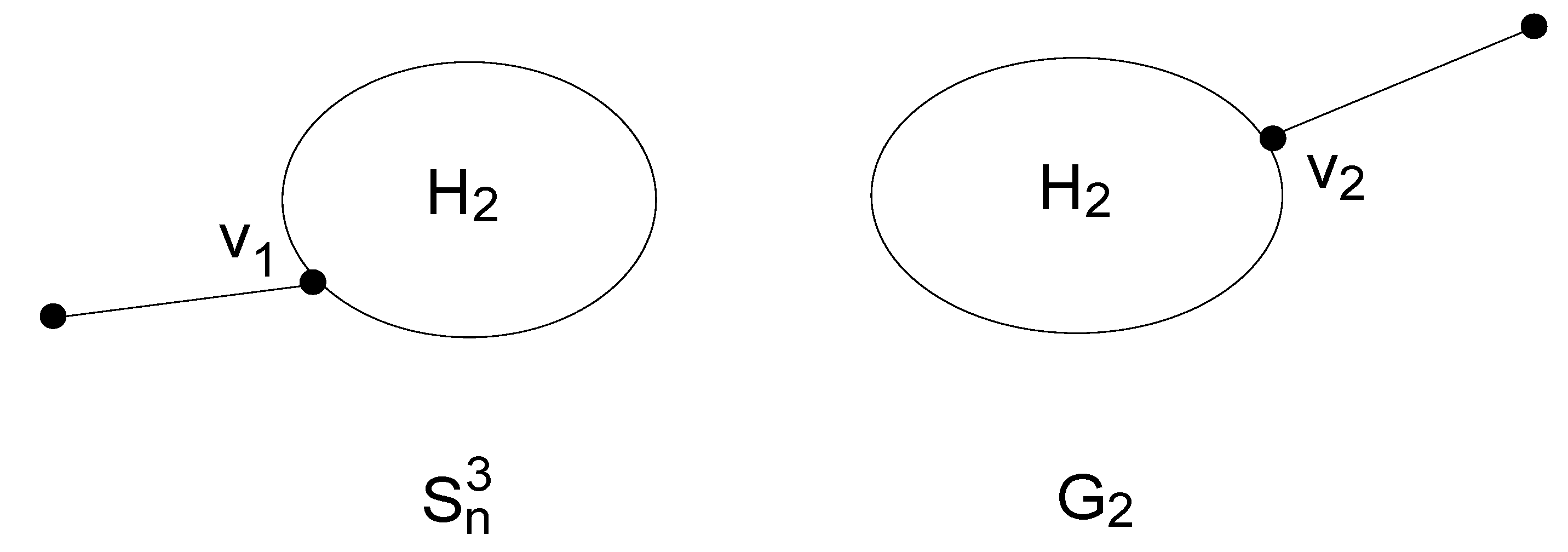
By Lemmas 2 and 3 and Equation (2) of the proof of Theorem 1, we can conclude that for $n\ge 16$ G which has the second-largest Resistance-Harary index in $\mathcal{U}\left(n\right)$ and those must be one of the graphs $G_1,G_2$, and $G_3\left(S_n^4\right)$, as shown in Figure 3.

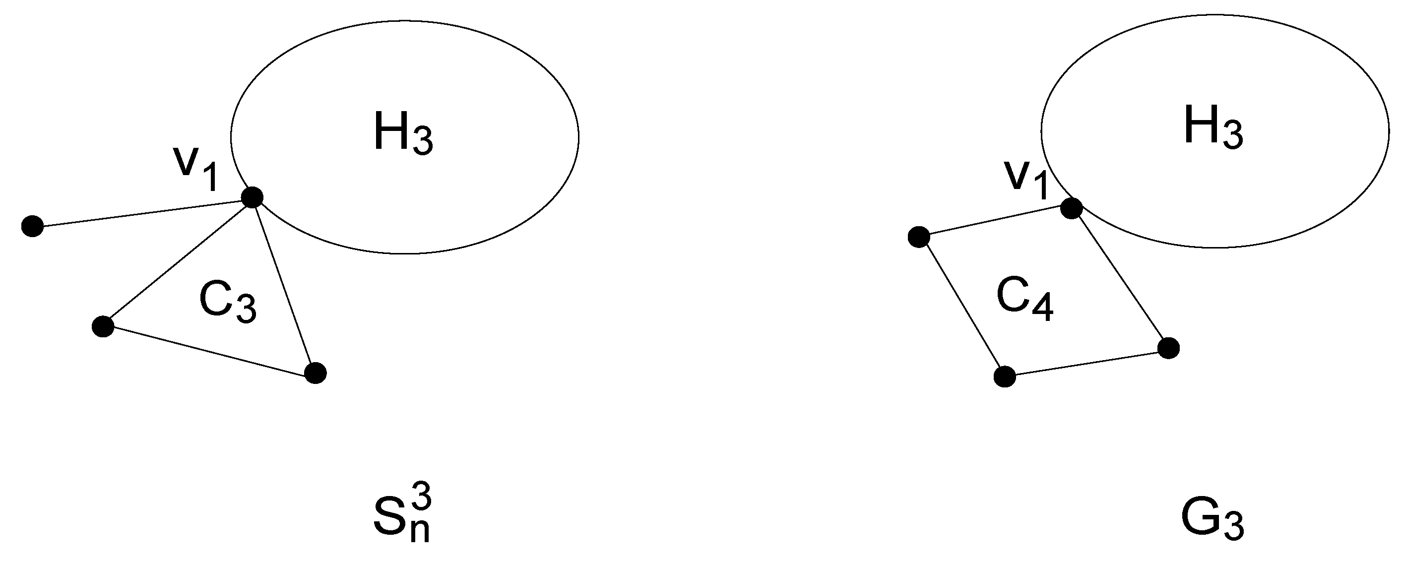
Theorem 3.

If $G\in \mathcal{U}\left(n\right)$, let ${max}^{*}\left\{RH\left(G\right)\right\}$ denote the second-largest Resistance-Harary index of graph G, then

$$\underset{G\in \mathcal{U}\left(n\right)}{ma{x}^{*}}\left\{RH\left(G\right)\right\}=\left\{\begin{array}{cc}\hfill RH\left(S_n^{n-1}\right)& ifn\le 7,\hfill \\ \hfill RH\left(S_n^4\right)& ifn=8,\hfill \\ \hfill RH\left(S_n^5\right)& ifn=9,10,\hfill \\ \hfill RH\left(S_n^3\right)& if11\le n\le 15,\hfill \\ \hfill RH\left(S_n^4\right)& ifn\ge 16.\hfill \end{array}\right.$$

Proof. 

(i) For $n\ge 16$.

Case 1. Let $H_1$ be the common subgraph of $S_n^3$ and $G_1$. Thus, we can view graphs $S_n^3$ and $G_1$ as the graphs depicted in Figure 4.

Then, we have

$$\begin{array}{c}\hfill \begin{array}{cc}\hfill RH\left(S_n^3\right)& =RH\left(H_1\right)+\frac{1}{2}+2\sum _{x\in H_1}\frac{1}{1+r(x,v_1)}\hfill \\ & =RH\left(H_1\right)+\frac{1}{2}+2\left[1+\frac{n-5}{2}+\frac{6}{5}\right],\hfill \\ \hfill RH\left(G_3\right)& =RH\left(H_1\right)+1+\sum _{x\in H_2}\frac{1}{1+r(x,v_1)}+\sum _{x\in H_2}\frac{1}{2+r(x,v_1)}\hfill \\ & =RH\left(H_1\right)+1+\left(1+\frac{6}{5}+\frac{n-5}{2}+\frac{1}{2}+\frac{n-5}{3}+\frac{3}{4}\right).\hfill \end{array}\end{array}$$

Therefore, we can get the difference

$$\begin{array}{c}\hfill \begin{array}{c}\hfill RH\left(S_n^3\right)-RH\left(G_1\right)=\frac{n}{6}-\frac{23}{60}.\end{array}\end{array}$$

Case 2. Let $H_2$ be the common subgraph of $S_n^3$ and $G_2$. Thus, we can view graphs $S_n^3$ and $G_2$ as the graphs depicted in Figure 5.

Then, we have

$$\begin{array}{c}\hfill \begin{array}{cc}\hfill RH\left(S_n^3\right)& =RH\left(S_n^3\right)+\sum _{x\in H_2}\frac{1}{1+r(x,v_1)}\hfill \\ & =RH\left(H_2\right)+\left[1+\frac{n-4}{2}+\frac{6}{5}\right],\hfill \\ \hfill RH\left(G_2\right)& =RH\left(H_2\right)+\sum _{x\in H_2}\frac{1}{1+r(x,v_2)}\hfill \\ & =RH\left(H_2\right)+\left[1+\frac{3(n-4)}{8}+\frac{6}{5}\right].\hfill \end{array}\end{array}$$

Therefore, we can get the difference

$$\begin{array}{c}\hfill \begin{array}{c}\hfill RH\left(S_n^3\right)-RH\left(G_2\right)=\frac{n}{8}-\frac{1}{2}.\end{array}\end{array}$$

Case 3. Let $H_3$ be the common subgraph of $S_n^3$ and $G_3$. Thus, we can view graphs $S_n^3$ and $G_3$ as the graphs depicted in Figure 6.

Then, we have

$$\begin{array}{c}\hfill \begin{array}{cc}\hfill RH\left(S_n^3\right)& =RH\left(H_3\right)+RH\left(S_4^3\right)+\sum _{x\in H_3,y\in S_4^3}\frac{1}{r(x,y)}\hfill \\ & =RH\left(H_3\right)+\frac{67}{10}+\frac{27(n-4)}{10},\hfill \\ \hfill RH\left(G_3\right)& =RH\left(H_3\right)+RH\left(C_4\right)+\sum _{x\in H_3,y\in C_4}\frac{1}{r(x,y)}\hfill \\ & =RH\left(H_3\right)+\frac{22}{3}+\frac{37(n-4)}{14}.\hfill \end{array}\end{array}$$

Therefore, we can get the difference

$$\begin{array}{c}\hfill \begin{array}{c}\hfill RH\left(S_n^3\right)-RH\left(G_3\right)=\frac{2n}{35}-\frac{181}{210}.\end{array}\end{array}$$

By the above expressions for the Resistance-Harary index of $G_1$, $G_2$ and $G_3$, we immediately have the desired result.

(ii) For $9\le n\le 15$.

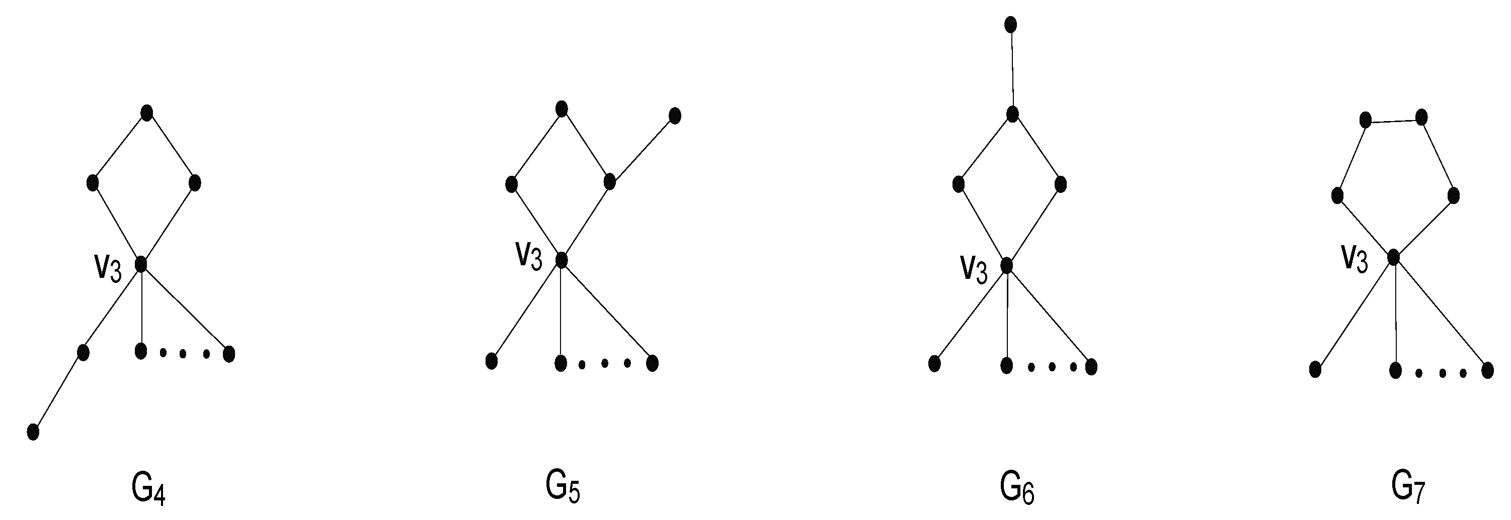
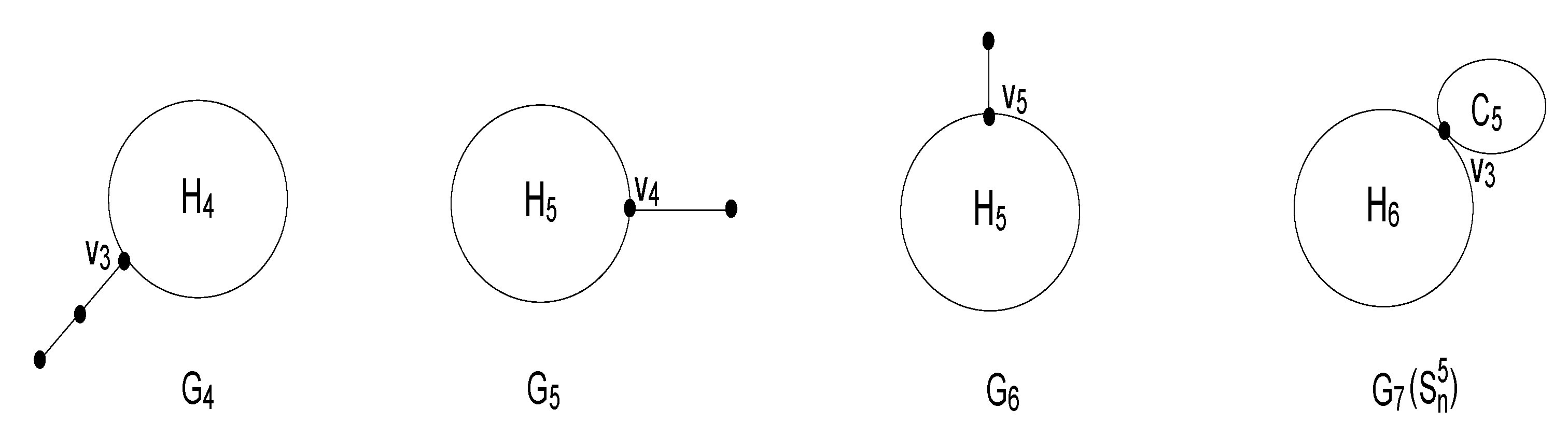
By the same arguments as used in (i), we conclude that the possible candidates having the second-largest Resistance-Harary index must be one of the graphs $G_4$, $G_5$, $G_6$, $G_7\left(S_n^5\right)$ (as shown in Figure 7) and $S_n^3$.

Let $H_4,H_5,H_6$ denote the common subgraphs of $S_n^4$ and $G_4-G_7$, respectively. Thus, we can view graphs $G_4-G_7$ as the graphs depicted in Figure 8.

Then, in a similar way, we have

$$\left\{\begin{array}{c}RH\left(S_n^4\right)-RH\left(G_4\right)=\frac{n}{6}-\frac{193}{462},\\ RH\left(S_n^4\right)-RH\left(G_5\right)=\frac{3n}{22}-\frac{15}{22},\\ RH\left(S_n^4\right)-RH\left(G_6\right)=\frac{n}{6}-\frac{5}{6},\\ RH\left(S_n^4\right)-RH\left(G_7\right)=\frac{85n}{693}-\frac{2921}{2772}.\end{array}\right.$$

Therefore, we have $HR\left(G_4\right)<HR\left(G_6\right)<HR\left(G_5\right)<HR\left(G_7\right)$. In connection with Equation (2), we have $G_7\left(S_n^5\right)<S_n^3$ if $11\le n\le 15$, so for $11\le n\le 15$, $S_n^3$ is the second largest. For $n=9,10$, in connection with Equation (2), we have $S_n^5$ is the second largest.

(iii) For $n\le 7$ and $n=8$.

In connection with Equation (2), we have $S_n^{n-1}$, $S_n^4$ is the second largest, respectively.

The result follows. □

4. Application

Now, we give a specific application of formation mentioned in the Section 3. Fully loaded graphs as a special class of unicyclic graphs also have some special properties about Resistance-Harary index. In this section, we determine the largest Resistance-Harary index among all fully loaded unicyclic graphs.

By a sequence of $\alpha$ and $\beta$ transformations to a fully loaded graph G, we can obtain a new graph, denoted by $Q_n^l$, which is obtained by attaching a pendent edge to each vertex of the unique cycle $C_l$ and attaching $n-2l+1$ pendent edges to a vertex of $C_l$. Then, by Lemma 2 and Corollary 1, we arrive at,

Theorem 4.

$G\in \mathfrak{U}(n;g)$, then $RH\left(G\right)\le RH\left(Q_n^g\right)$.

Next, we determine the graph in $\mathfrak{U}\left(n\right)$ with the largest Resistance-Harary index.

Theorem 5.

If $G\in \mathfrak{U}\left(n\right)$, then

$$\underset{G\in \mathfrak{U}\left(n\right)}{max}\left\{RH\left(G\right)\right\}=\left\{\begin{array}{cc}\hfill RH\left(Q_n^3\right)& ifn\le 7,\hfill \\ \hfill RH\left(Q_n^4\right)& ifn=8,9,\hfill \\ \hfill RH\left(Q_n^3\right)& ifn\ge 10.\hfill \end{array}\right.$$

Proof. 

Using a similar way as in Section 3.2, we can conclude that the unicyclic graphs with $n\ge 16$ in Figure 9 have the second largest or third largest Resistance-Harary index.

Only one graph $Q_n^3$ is fully loaded (Graph 9 in Figure 9). Thus, $Q_n^3$ has the largest Resistance-Harary index among all fully loaded graphs with $n\ge 16$. For $n\le 15$, from Lemmas 2 and 3 we can conclude that the fully loaded graph with largest Resistance-Harary index must be one of the five situations $Q_n^3,Q_n^4,Q_n^5,Q_n^6,Q_n^7$.

For completeness of the proof, we list all possible values as follows. For $n\le 7$, there is only one situation $Q_7^3$ with $n=7$ and $Q_6^3$ with $n=6$, so we begin at $n=8$.

Case 1.$n=8$.

$$\begin{array}{c}\hfill \begin{array}{cc}\hfill RH\left(Q_8^3\right)=19.625,& RH\left(Q_8^4\right)=20.026.\hfill \end{array}\end{array}$$

Then, $\underset{G\in \mathfrak{U}\left(n\right)}{max}\left\{RH\left(G\right)\right\}=RH\left(Q_8^4\right)$.

Case 2.$n=9$.

$$\begin{array}{c}\hfill \begin{array}{cc}\hfill RH\left(Q_9^3\right)=24.075,& RH\left(Q_9^4\right)=24.229.\hfill \end{array}\end{array}$$

Then, $\underset{G\in \mathfrak{U}\left(n\right)}{max}\left\{RH\left(G\right)\right\}=RH\left(Q_9^4\right)$.

Case 3.$n=10$.

$$\begin{array}{c}\hfill \begin{array}{cc}\hfill RH\left(Q_{10}^3\right)=& 29.025,RH\left(Q_{10}^4\right)=28.933,RH\left(Q_{10}^5\right)=28.866.\hfill \end{array}\end{array}$$

Then, $\underset{G\in \mathfrak{U}\left(n\right)}{max}\left\{RH\left(G\right)\right\}=RH\left(Q_{10}^3\right)$.

Case 4.$n=11$.

$$\begin{array}{c}\hfill \begin{array}{cc}\hfill RH\left(Q_{11}^3\right)=& 34.475,RH\left(Q_{11}^4\right)=34.136,RH\left(Q_{11}^5\right)=33.725.\hfill \end{array}\end{array}$$

Then, $\underset{G\in \mathfrak{U}\left(n\right)}{max}\left\{RH\left(G\right)\right\}=RH\left(Q_{11}^3\right)$.

Case 5.$n=12$.

$$\begin{array}{c}\hfill \begin{array}{cc}\hfill RH\left(Q_{12}^3\right)=& 40.425,RH\left(Q_{12}^4\right)=39.840,RH\left(Q_{12}^5\right)=39.085,RH\left(Q_{12}^6\right)=38.563.\hfill \end{array}\end{array}$$

Then, $\underset{G\in \mathfrak{U}\left(n\right)}{max}\left\{RH\left(G\right)\right\}=RH\left(Q_{12}^3\right)$.

Case 6.$n=13$.

$$\begin{array}{c}\hfill \begin{array}{ccc}\hfill RH\left(Q_{13}^3\right)=& 46.875,RH\left(Q_{13}^4\right)=46.043,RH\left(Q_{13}^5\right)=44.944,RH\left(Q_{13}^6\right)=\hfill & 44.003.\end{array}\end{array}$$

Then, $\underset{G\in \mathfrak{U}\left(n\right)}{max}\left\{RH\left(G\right)\right\}=RH\left(Q_{13}^3\right)$.

Case 7.$n=14$.

$$\begin{array}{c}\hfill \begin{array}{cc}\hfill RH\left(Q_{14}^3\right)=& 53.825,RH\left(Q_{14}^4\right)=52.747,RH\left(Q_{14}^5\right)=51.303,\hfill \\ \hfill RH\left(Q_{14}^6\right)=& 49.942,RH\left(Q_{14}^7\right)=49.987.\hfill \end{array}\end{array}$$

Then, $\underset{G\in \mathfrak{U}\left(n\right)}{max}\left\{RH\left(G\right)\right\}=RH\left(Q_{14}^3\right)$.

Case 8.$n=15$.

$$\begin{array}{c}\hfill \begin{array}{cc}\hfill RH\left(Q_{15}^3\right)=& 61.275,RH\left(Q_{15}^4\right)=59.950,RH\left(Q_{15}^5\right)=58.163,\hfill \\ \hfill RH\left(Q_{15}^6\right)=& 56.382,RH\left(Q_{15}^7\right)=54.946.\hfill \end{array}\end{array}$$

Then, $\underset{G\in \mathfrak{U}\left(n\right)}{max}\left\{RH\left(G\right)\right\}=RH\left(Q_{15}^3\right)$.

The proof is completed. □

5. Conclusions

This paper focuses on Resistance-Harary index in unicyclic graphs. Let $\mathcal{U}\left(n\right)$ and $\mathfrak{U}\left(n\right)$ be the set of unicyclic graphs and fully loaded unicyclic graphs, respectively. Here, we first give a more precise proof about the largest Resistance-Harary index among all unicyclic graphs, then determine the graph of $\mathcal{U}\left(n\right)$ with second-largest Resistance-Harary index and apply this way to fully loaded unicyclic graphs determine the graph of $\mathfrak{U}\left(n\right)$ with largest Resistance-Harary index.

References

- Klein, D.J.; Randić, M. Resistance distance. J. Math. Chem. 1993, 12, 81–95. [Google Scholar] [CrossRef]
- Du, J.; Su, G.; Tu, J.; Gutman, I. The degree resistance distance of cacti. Discrete Appl. Math. 2015, 188, 16–24. [Google Scholar] [CrossRef]
- Bu, C.; Yan, B.; Zhou, X.; Zhou, J. Resistance distance in subdivision-vertex join and subdivision-edge join of graphs. Linear Algebra Appl. 2014, 458, 454–462. [Google Scholar] [CrossRef]
- Feng, L.H.; Yu, G.; Liu, W. Futher results regarding the degree Kirchhoff index of a graph. Miskolc Math. Notes 2014, 15, 97–108. [Google Scholar] [CrossRef]
- Feng, L.H.; Yu, G.; Xu, K.; Jiang, Z. A note on the Kirchhoff index of bicyclic graphs. ARS Combin. 2014, 114, 33–40. [Google Scholar]
- Gao, X.; Luo, Y.; Liu, W. Resistance distance and the Kirchhoff index in Cayley graphs. Discrete Appl. Math. 2011, 159, 2050–2057. [Google Scholar] [CrossRef]
- Gao, X.; Luo, Y.; Liu, W. Kirchhoff index in line, subdivision and total graphs of a regular graph. Discrete Appl. Math. 2012, 160, 560–565. [Google Scholar] [CrossRef]
- Gutman, I.; Feng, L.; Yu, G. On the degree resistance distance of unicyclic graphs. Trans. Comb. 2012, 1, 27–40. [Google Scholar]
- Liu, J.; Pan, X.; Yu, L.; Li, D. Complete characterization of bicyclic graphs with minimal Kirchhoff index. Discrete Appl. Math. 2016, 200, 95–107. [Google Scholar] [CrossRef]
- Liu, J.; Wang, W.; Zhang, Y.; Pan, X. On degree resistance distance of cacti. Discrete Appl. Math. 2016, 203, 217–225. [Google Scholar] [CrossRef]
- Liu, J.; Pan, X. Minimizing Kirchhoff index among graphs with a given vertex bipartiteness. Appl. Math. Comput. 2016, 291, 84–88. [Google Scholar] [CrossRef]
- Pirzada, S.; Ganie, H.A.; Gutman, I. On Laplacian-Energy-Like Invariant and Kirchhoff Index. MATCH Commun. Math. Comput. Chem. 2015, 73, 41–59. [Google Scholar]
- Plavšić, D.; Nikolić, S.; Mihalić, Z. On the Harary index for the characterization of chemical graphs. J. Math. Chem. 1993, 12, 235–250. [Google Scholar]
- Ivanciuc, O.; Balaban, T.S.; Balaban, A.T. Reciprocal distance matrix, related local vertex invariants and topological indices. J. Math. Chem. 1993, 12, 309–318. [Google Scholar] [CrossRef]
- Furtula, B.; Gutman, I.; Katanić, V. Three-center Harary index and its applications. Iranian J. Math. Chem. 2016, 7, 61–68. [Google Scholar]
- Feng, L.H.; Lan, Y.; Liu, W.; Wang, X. Minimal Harary index of graphs with samll parameters. MATCH Commun. Math. Comput. Chem. 2016, 76, 23–42. [Google Scholar]
- Li, X.; Fan, Y. The connectivity and the Harary index of a graph. Discrete Appl. Math. 2015, 181, 167–173. [Google Scholar] [CrossRef]
- Xu, K.; Das, K.C. On Harary index of graphs. Discrete Appl. Math. 2011, 159, 1631–1640. [Google Scholar] [CrossRef]
- Xu, K. Trees with the seven smallest and eight greatest Harary indices. Discrete Appl. Math. 2012, 160, 321–331. [Google Scholar] [CrossRef]
- Xu, K.; Das, K.C. Extremal unicyclic and bicyclic graphs with respect to Harary index. Bull. Malays. Math. Sci. Soc. 2013, 36, 373–383. [Google Scholar]
- Xu, K.; Wang, J.; Das, K.C.; Klavžar, S. Weighted Harary indices of apex trees and k-apex trees. Discrete Appl. Math. 2015, 189, 30–40. [Google Scholar] [CrossRef]
- Yu, G.; Feng, L. On the maximal Harary index of a class of bicyclic graphs. Util. Math. 2010, 82, 285–292. [Google Scholar]
- Chen, S.B.; Guo, Z.J.; Zeng, T.; Yang, L. On the Resistance-Harary index of unicyclic graphs. MATCH Commun. Math. Comput. Chem. 2017, 78, 189–198. [Google Scholar]
- Wang, H.; Hua, H.; Zhang, L.; Wen, S. On the Resistance-Harary Index of Graphs Given Cut Edges. J. Chem. 2017, 2017, 3531746. [Google Scholar] [CrossRef]
© 2019 by the authors. Licensee MDPI, Basel, Switzerland. This article is an open access article distributed under the terms and conditions of the Creative Commons Attribution (CC BY) license (http://creativecommons.org/licenses/by/4.0/).