Abstract
In this paper, stability analysis of a fractional-order linear system described by the Caputo–Fabrizio (CF) derivative is studied. In order to solve the problem, character equation of the system is defined at first by using the Laplace transform. Then, some simple necessary and sufficient stability conditions and sufficient stability conditions are given which will be the basis of doing research of a fractional-order system with a CF derivative. In addition, the difference of stability domain between two linear systems described by two different fractional derivatives is also studied. Our results permit researchers to check the stability by judging the locations in the complex plane of the dynamic matrix eigenvalues of the state space.
1. Introduction
Recently, fractional-order systems have gained increasing interests. Research into fractional-order systems has become a hot subject because of many advantages of fractional derivatives. The especially important advantages of the dynamic systems with fractional derivatives are the following two facts. First, researchers have more degrees of freedom in the model and memories of various materials and processes are included in the model, see [1,2,3,4]. Second, fractional-order controllers have been designed to enhance the robustness and the performance of the closed loop control system, such as CRONE controller [5], TID controller [6] and fractional PID controller [7].
So far, powerful criteria of fractional-order systems have been proposed. The most well-known one is Matignon’s stability theorem [8]. It permits us to check the stability by judging the locations in the complex plane of the dynamic matrix eigenvalues of the state space. Matignon’s theorem is the starting point of several useful and important results in the field. In addition, LMI approach [9,10,11] and Lyapunov approach [12,13] are also used to investigate the stability of fractional order linear time invariant systems. Analysis of equations generated by different fractional derivatives have been done, see [14].
Recently, a new definition of the fractional derivative without a singular kernel has been proposed by Caputo and Fabrizio in 2015 [15]. This new fractional derivative is less affected by past, compared with the classical Caputo fractional derivative which shows a slow stabilization. This new derivative has gained widely attention. Paper [16] not only justified that CF derivative are much more need to describe the real problems and presented some good examples as well. In addition, ref. [17] studied the kernel and no-index property of CF derivative separately, which help us to know more information of the derivative and its links to other fractional derivative and real problems. But there is not a method applicable to all linear systems described by this new derivative.
In this paper, first, problem formulation and preliminaries are presented. Then, we mainly study the stability of fractional-order linear system. By using the Laplace transform, characteristic equation for the system is established, some simple necessary and sufficient stability conditions and sufficient stability conditions are deserved. we also studied the Stable domains relations between two linear systems described by two different derivative. Finally, an example is provided to demonstrate the effectiveness of our results. The characteristic equation in this paper can be extended to all linear fractional-order systems described by the CF derivative. Theorems in this paper can also be used to analyse local stability of nonlinear system described by the CF derivative.
2. Problem Formulation and Preliminaries
The differ-integral operator, denoted by , is a combined differentiation and integration operator commonly used in fractional calculus which is defined by:
There are different definitions for fractional derivatives. The most commonly used definition is the classical Caputo. In the rest of the paper, is used to denote the classical Caputo fractional derivative of order
where m is an integer satisfying .
Caputo and Fabrizio proposed a new fractional derivative in 2015 [15]. In this paper, is used to denote this new fractional derivative of order
where . This new fractional derivative is less affected by the past, compared with the which shows a slow stabilization.
In this paper, we consider the following fractional-order linear system described by the Caputo–Fabrizio derivative
where , , .
Next, a character equation of this system will be established and some simple stability conditions will be given.
3. Main Results
In this section, we studied the stability of a fractional-order linear system (3) described by the Caputo–Fabrizio derivative, and compared the stability domains of the system described by two different fractional derivative.
3.1. Stability of Fractional-Order Linear System (3) Described by the Caputo–Fabrizio Derivative
Definition 1
([8]). The autonomous system (3), with , is said to be asymptotically stable if and only if
In order to solve system (3), using Laplace transform [18] for a given initial condition , we note that
where . Simplify (4), we get
Set , Equation (5) is written as
Since, the distribution of ’s eigenvalues totally determines the stability of system (3), so the following definition is obvious.
Definition 2.
The character equation of system (3) is
Remark 1.
If we consider the same system described by Caputo derivative, then its character equation is
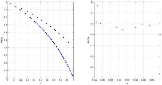
It is difficult to solve it since this is a fractional order equation. In addition, without loss of generality, the following figure shows the relations between real part of s and α. Let . Figure 1 below illustrates that is less affected by α, therefore the result described by the new derivative is better than the one described by the Caputo derivative.
Figure 1.
Relations between Re(s) and (left is , right is Equation (7)).
Theorem 1.
Proof.
So, , if and only if the real parts of the eigenvalues of the matrix are negative. That is , if and only if the real parts of the roots of the equation
are negative.
This proved this theorem. □
Remark 2.
Theorem 1 means all eigenvalues of matrix are negative. By this way, the LMI where , can be used to analysis the stability of system (3).
Theorem 2.
The system (3) is asymptotically stable if and only if the eigenvalues of the matrix A satisfy .
Proof.
Since , then is invertible. Employing the well-known relation , we can get
Set the eigenvalues of matrix A are , then the eigenvalues of matrix are
If , that is , According to Theorem 1, this theorem is proved. □
Corollary 1.
The system (3) is asymptotically stable if eigenvalues of the matrix A satisfy one of the following conditions:
Proof.
Modify the necessary and sufficient stability condition in Theorem 2, we obtain
So, the dividing line between stable domain and unstable domain is the circle
Thus, the conclusions can be easily obtained. □
Remark 3.
Nonlinear systems are usually needed to describe the real problems. Study of local stability of equilibrium points is very important for nonlinear systems. As method of local stability of equilibrium points is local linearization, all the theorems and Corollaries can be used to study the local stability of equilibrium points of nonlinear systems.
3.2. Stable Domains Relations between Two Linear Systems Described by Two Different Derivative
In this section, we will discuss the stable domains relations between system (3) and the following system
where is the classical Caputo derivative.
Theorem 3
([8]). System (13) with and is asymptotically stable if and only if , where is the spectrum (set of all eigenvalues) of A.
Next, stable and unstable domain relations and the difference between system (3) and (13) are shown by the following two figures (see Figure 2 and Figure 3).
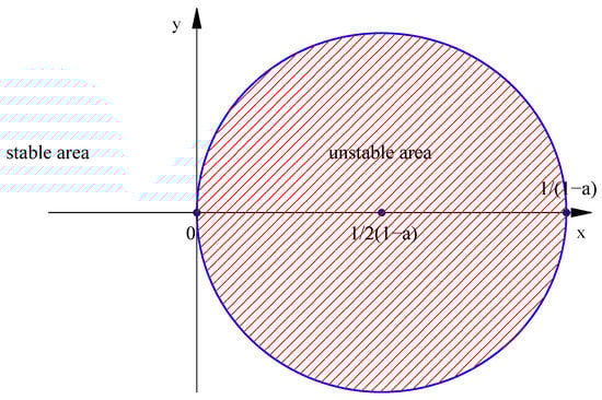
Figure 2.
Stability domain and unstability domain of system (3).
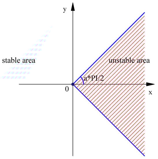
Figure 3.
Stability domain and unstability domain of system (13).
According to Figure 2, the unstable domain of the system (3) is a bounded closed region which is a circle with a radius of . The center of the circle is . With the increase of fractional-order , the scope of the unstable region becomes larger and larger.
However, from Figure 3, the unstable domain of the system (13) is an unbound convex region. With the increase of fractional-order , the scope of the unstable region becomes larger and larger.
The unstable domains of these two systems have overlapping parts. The two systems have their own advantages and disadvantages, but obviously, the scope of the unstable region of system (3) is much smaller than that of system (13).
Remark 4.
In this paper, the fractional-order α is within the interval for some theorems. If α is without the interval , theorems and corollaries can not be used. In addition, the condition that is invertible is also needed.
4. Numerical Examples
Example 1.
Consider the stability of the following fractional-order system
described by the Caputo–Fabrizio derivative and the Caputo derivative separately. Let
Eigenvalues of matrix A are .
First, we consider that the system is described by the Caputo–Fabrizio derivative.
Three cases of fractional-order with three different values are discussed, see Figure 4, Figure 5 and Figure 6.
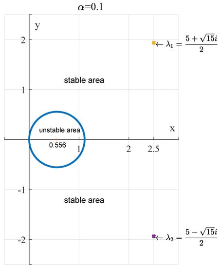
Figure 4.
When , system (14) is stable.
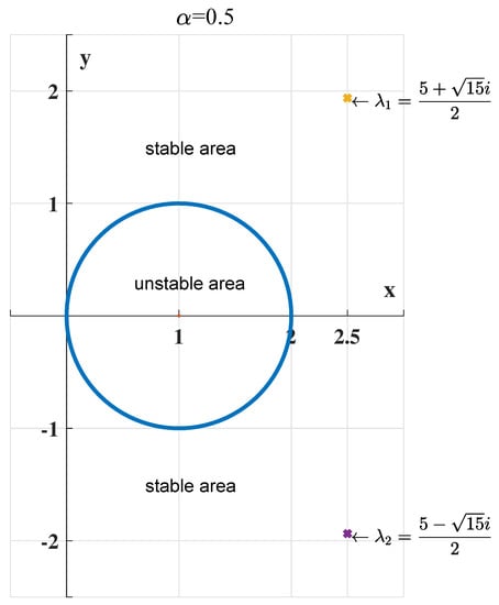
Figure 5.
When , system (14) is stable.
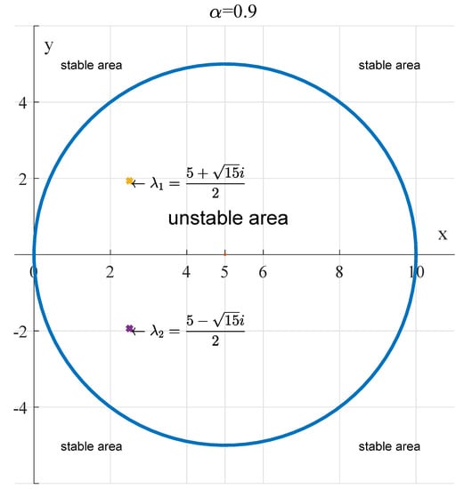
Figure 6.
When , system (14) is unstable.
Actually,
According to Theorem 2, for all , this system is asymptotically stable, which also shows that our results are accurate.
Next, we consider the system described by the Caputo derivative with
According to Theorem 3, for all , the system is asymptotically stable. The domain of that makes the system described by the Caputo derivative stable is obviously much narrower than the system described by the Caputo–Fabrizio derivative.
5. Conclusions
By using Laplace transformation, this paper mainly presents some brief, necessary, and sufficient conditions, and some sufficient conditions for the stability of fractional-order linear system described by the CF derivative. The fractional-order systems with CF derivative are needed to describe the real system, more so than the systems with other fractional derivatives. Theorems in this paper not only permit researchers to check the stability of the system through the location in the complex plane of the dynamic matrix eigenvalues of the state space, but also can help to study the other systems with CF derivatives, like prey–predator systems, HIV/AIDS systems, and fractional-order complex networks, etc.
Author Contributions
Conceptualization, S.-M.Z.; Funding acquisition, H.L.; Supervision, H.-B.L. and S.-M.Z.; Writing—original draft, J.C. and H.L.; and Writing—review and editing, H.L. and H.-B.L.
Funding
This work was financially supported by the National Natural Science Foundation of China (11271001, 11101071), and the Fundamental Research Funds for the Central Universities(ZYGX2016J131, ZYGX2016J138).
Acknowledgments
The authors would like to thank reviewers and editors for providing us some good suggestions and help.
Conflicts of Interest
The authors declare no conflict of interest.
References
- Khalil, R.; Al Horani, M.; Yousef, A.; Sababheh, M. A new definition of fractional derivative. J. Comput. Appl. Math. 2014, 264, 65–70. [Google Scholar] [CrossRef]
- Podlubuy, I. Fractional Differential Equations; Khalil, R., Al Horani, M., Yousef, A., Sababheh, M., Eds.; Academic Press: Cambridge, MA, USA, 1999. [Google Scholar]
- Side, O. Electromagnetic Theory; Chelsea: New York, NY, USA, 1971. [Google Scholar]
- Ita, J.J.; Stixrude, L. Petrology, elasticity, and composition of the mantle transition zone. J. Geophys. Res. 1992, 97, 6849–6866. [Google Scholar] [CrossRef]
- Oustaloup, A.; Morean, X.; Nouiuant, M. The CRONE suspension. Control Eng. Pract. 1996, 4, 1101–1108. [Google Scholar] [CrossRef]
- Lurie, B.J. Tunable TID Controller. U.S. Patent 5, 371, 630, 6 December 1944. [Google Scholar]
- Podlubuy, I. Fractional-order systems and PIλDu-controllers. IEEE Trans. Autom. Control 1999, 44, 208–214. [Google Scholar] [CrossRef]
- Matignon, D. Stability results on fractional differential equations to control processing. In Proceedings of the Computational Engineering in Syatems and Application Multiconference; IMACS, IEEE-SMC: Lille, France, 1996; Volume 2, pp. 963–968. [Google Scholar]
- Sheng, Y.X.; Lu, J.G. Robust stability and stabilization of fractional-order linear systems with nonlinear ncertain parameters: An LMI approach. Chaos Solitons Fractals 2009, 42, 1163–1169. [Google Scholar]
- Sabatier, J.; Moze, M.; Farges, C. LMI stability conditions for fractional order systems. Comput. Math. Appl. 2010, 59, 1594–1609. [Google Scholar] [CrossRef]
- Lu, J.G.; Chen, Y.Q. Robust stability and stabilization of fractional-order interval systems with the Fractional Order α: The 0 < α < 1 Case. IEEE Trans. Autom. Control 2010, 55, 152–158. [Google Scholar]
- Ahn, H.S.; Chen, Y.Q.; Podlubny, I. Robust stability test of a class of linear time-invariant interval fractional-order system using Lypunov inequality. Appl. Math. Comput. 2007, 187, 27–34. [Google Scholar]
- Trigeassou, J.C.; Maamri, N.; Sabatier, J.; Oustaloup, A. A Lyapunov approach to the stability of fractional differential equations. Signal Process. 2011, 91, 437. [Google Scholar] [CrossRef]
- Atangana, A. Non validity of index law in fractional calculus: A fractional differential operator with Markovian and non-Markovian properties. Phys. A Stat. Mech. Appl. 2018, 505, 688–706. [Google Scholar] [CrossRef]
- Caputo, M.; Fabrizio, M. A new definition of fractional derivative without singular kernel. Prog. Fract. Differ. Appl. 2015, 2, 73–85. [Google Scholar]
- Atangana, A.; Gómez-Aguilar, J.F. Decolonisation of fractional calculus rules: Breaking commutativity and associativity to capture more natural phenomena. Eur. Phys. J. Plus 2018, 133, 166. [Google Scholar] [CrossRef]
- Atangana, A. Blind in a commutative world: Simple illustrations with functions and chaotic attractors. Chaos Solitons Fractals 2018, 114, 347–363. [Google Scholar] [CrossRef]
- Mashayekhizadeh, V.; Dejam, M.; Ghazanfari, M.H. The application of numerical Laplace inversion methods for type curve development in well testing: A comparative study. Petrol. Sci. Technol. 2011, 29, 695–707. [Google Scholar] [CrossRef]
© 2019 by the authors. Licensee MDPI, Basel, Switzerland. This article is an open access article distributed under the terms and conditions of the Creative Commons Attribution (CC BY) license (http://creativecommons.org/licenses/by/4.0/).