Orthogonality Properties of the Pseudo-Chebyshev Functions (Variations on a Chebyshev’s Theme)

Abstract

The third and fourth pseudo-Chebyshev irrational functions of half-integer degree are defined. Their definitions are connected to those of the first- and second-kind pseudo-Chebyshev functions. Their orthogonality properties are shown, with respect to classical weights.

1. Introduction

In a recent article [1], starting from the complex Bernoulli spiral, the sets of classical Chebyshev polynomials of the first- and second-kind have been extended to the case of fractional indices. The resulting functions have been called pseudo-Chebyshev polynomials (or functions), since actually, they are not polynomials, but irrational functions. However, in the particular case of half-integer indices, the functions $T_{n+1/2}$, $U_{n+1/2}$ satisfy the same properties of their classical counterparts, including recurrence relations, differential equations, and orthogonality properties, as has been proven in [2].

In this article, after recalling the definitions of the third- and fourth-kind Chebyshev polynomials, we introduce the third- and fourth-kind pseudo-Chebyshev functions $V_{n+1/2}$, $W_{n+1/2}$, focusing our attention on the orthogonality properties satisfied by these new irrational functions.

Even though there are links to the classical Chebyshev polynomials, it seems unusual to find a set of irrational functions that satisfy properties so similar to their polynomial counterparts.

A clear possible application of the introduced functions is the expansion of irrational functions in non-trigonometric Fourier series, and-for the third-kind pseudo-Chebyshev functions-the construction of quadrature rules applied to functions whose singularities occur only at the end points (+1 and −1) (see [3] for similar situations). In Section 8, the connection with the Dirichlet kernel is shown, and in a forthcoming article, further properties derived from links to classical Chebyshev polynomials will be highlighted.

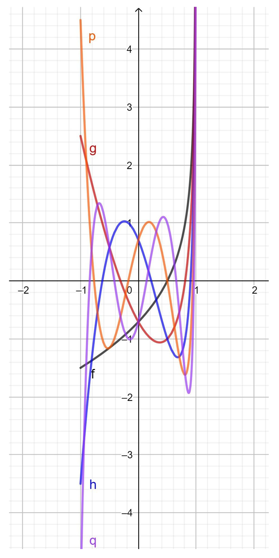
2. Chebyshev Polynomials

The Chebyshev polynomials of the first- and second-kind were introduced by Pafnuty L. Chebyshev in the 19th Century. They can be derived as the real and imaginary part of the exponential function $e^{in\theta }={(cos\theta +isin\theta )}^n$, setting $x=cos\theta$ and using the Euler formula (see [4] for details).

The first-kind Chebyshev polynomials are important in approximation theory and Gaussian quadrature rules. Indeed, by using their roots-called Chebyshev nodes-the resulting interpolation polynomial minimizes the Runge phenomenon. Furthermore, the relevant approximation is the best approximation to a continuous function under the maximum norm.

Linked with such polynomials are the Chebyshev polynomials of the second-kind, which appear in computing the powers of 2 × 2 non-singular matrices [5]. Generalizations of these polynomials have been also introduced, in particular for computing powers of higher order matrices (see, e.g., [6,7]).

An excellent book is [3]. The importance of these polynomial sets in applications is shown in [8].

It is also useful to notice that Chebyshev polynomials represent an important tool to derive integral representations [9,10], and that they can be generalized by using the properties and formalism of the Hermite polynomials [11], for instance by introducing multi-variable polynomials recognized as belonging to the Chebyshev family [12,13,14].

Recently, the Chebyshev polynomials of the first- and second-kind have been used in order to represent the real and imaginary part of complex Appell polynomials [15].

Other sets of orthogonal polynomials, linked to the above-mentioned ones, are known as the third- and fourth-kind Chebyshev polynomials.

The third- and fourth-kind Chebyshev polynomials have been studied and applied by several scholars (see, e.g., [16,17,18]), because they are useful in quadrature rules, when the singularities occur only at one of the end points +1 or −1 (see [3]). Furthermore, they have been recently applied in numerical analysis to solve high odd-order boundary-value problems with homogeneous or nonhomogeneous boundary conditions [17].

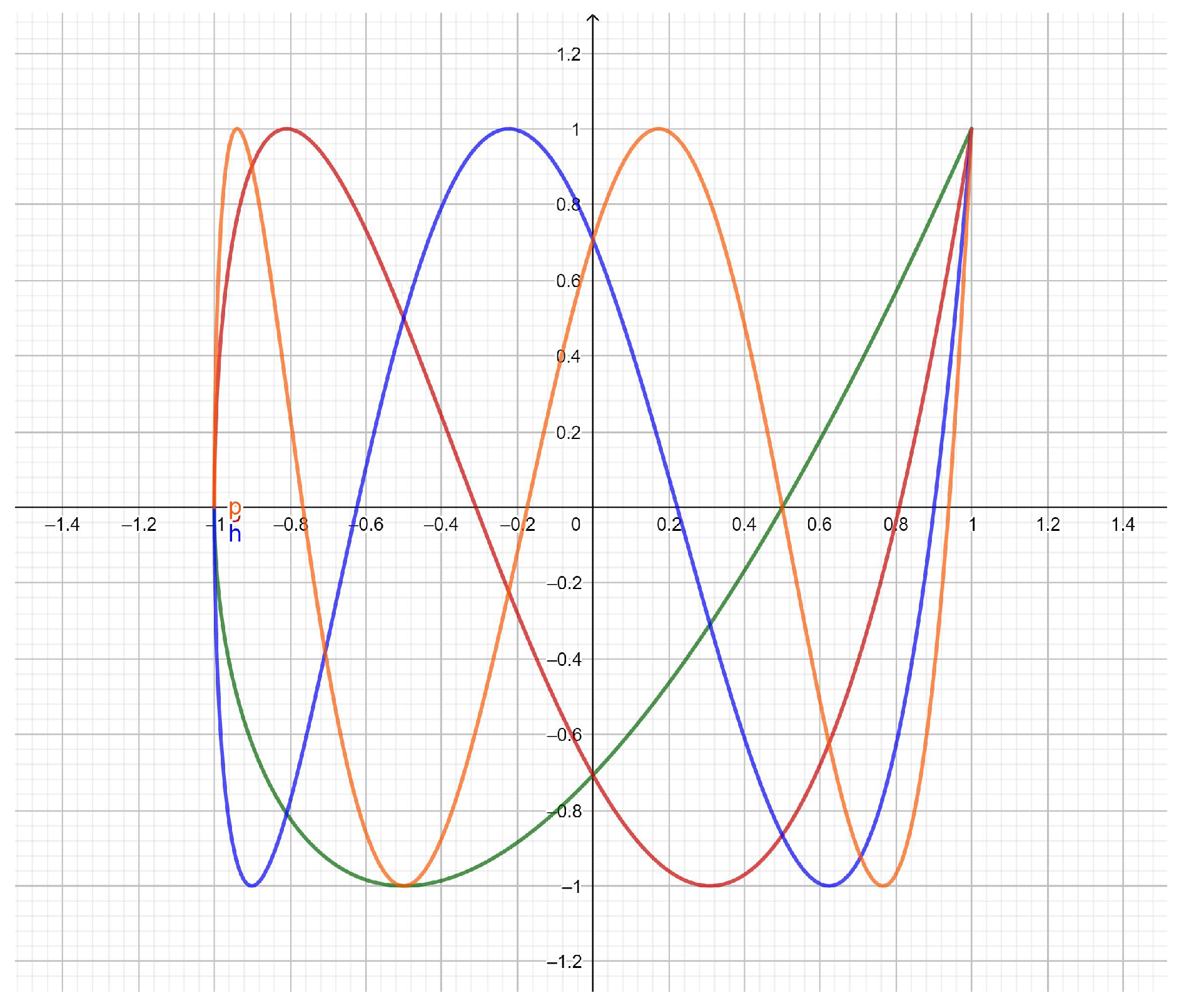
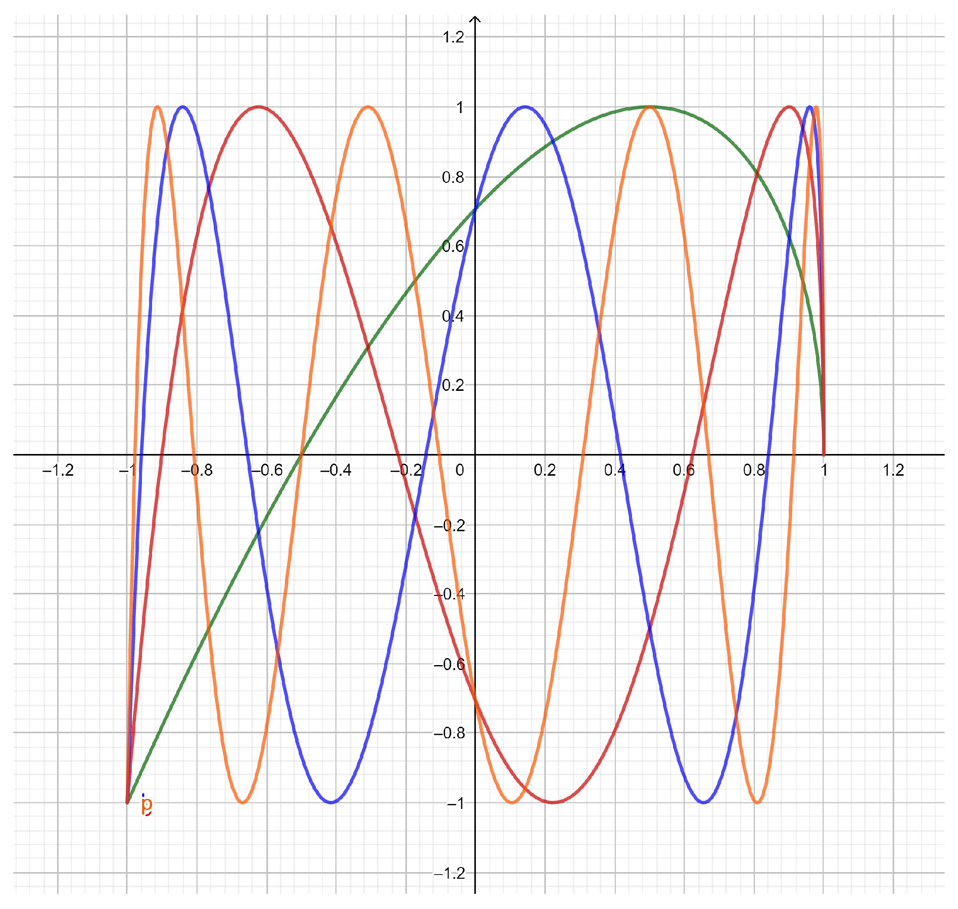
3. First- and Second-Kind Pseudo-Chebyshev Functions

Definitions

In [1,2], we introduced the following definitions:

• First-kind pseudo-Chebyshev functions (Figure 1):

  $$\begin{array}{c}\hfill \begin{array}{c}{T}_{k+\frac{1}{2}}(x)=cos\left((k+\frac{1}{2})arccos(x)\right)\end{array}\end{array}$$

  (1)
• Second-kind pseudo-Chebyshev functions (Figure 2):

  $$\begin{array}{c}\hfill \begin{array}{c}{U}_{k-\frac{1}{2}}(x)=\frac{sin\left((k+\frac{1}{2})arccos(x)\right)}{\sqrt{1-x^2}}.\end{array}\end{array}$$

  (2)

In [2], the main properties of these functions have been studied.

4. Third- and Fourth-Kind Chebyshev Polynomials

Definitions

• The third-kind Chebyshev polynomials (Figure 3) can be expressed in terms of the first-kind pseudo-Chebyshev functions as follows:

  $$\begin{array}{c}\hfill \begin{array}{c}{V}_k(x)=\frac{T_{k+\frac{1}{2}}(x)}{T_{1/2}(x)}=\sqrt{\frac{2}{1+x}}cos\left((k+\frac{1}{2})arccos(x)\right).\end{array}\end{array}$$

  (3)
• The fourth-kind Chebyshev polynomials (Figure 4) can be expressed in terms of the second-kind pseudo-Chebyshev functions as follows:

  $$\begin{array}{c}\hfill \begin{array}{c}{W}_k(x)=\frac{U_{k-\frac{1}{2}}(x)}{U_{1/2}(x)}=\sqrt{\frac{2}{1-x}}sin\left((k+\frac{1}{2})arccos(x)\right).\end{array}\end{array}$$

  (4)

The third- and fourth-kind Chebyshev polynomials satisfy the orthogonality property:

$$\begin{array}{c}\hfill \begin{array}{c}{\int }_{-1}^1{V}_h(x)V_k(x)\sqrt{\frac{1+x}{1-x}}dx={\int }_{-1}^1{W}_h(x)W_k(x)\sqrt{\frac{1-x}{1+x}}dx=\pi {\delta }_{h,k}.\end{array}\end{array}$$

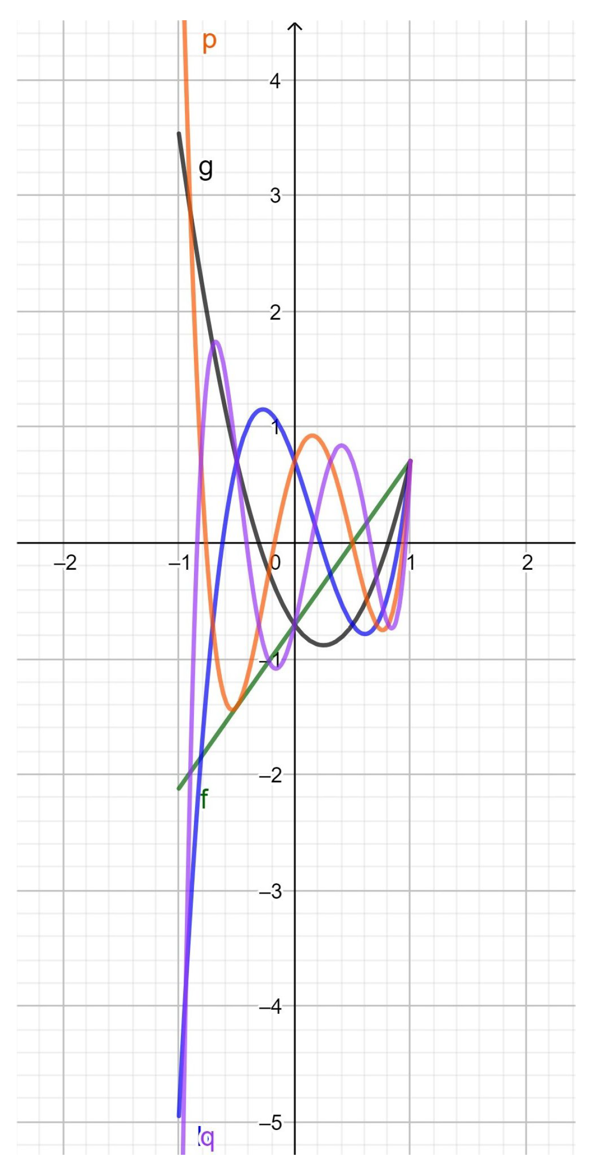
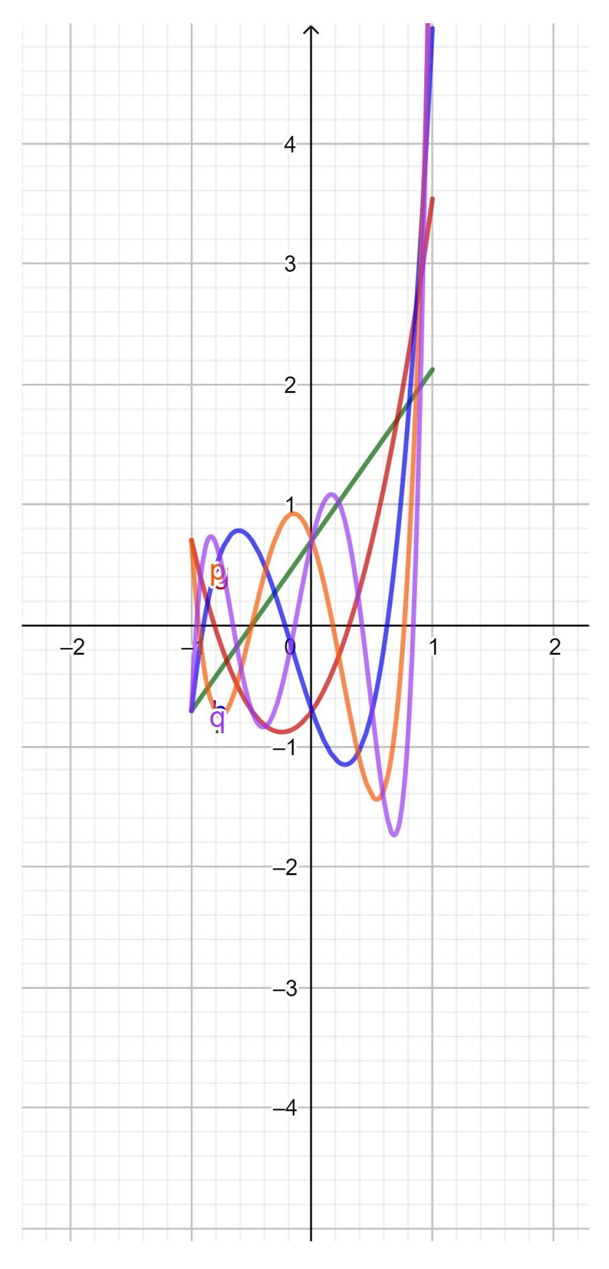
5. Third- and Fourth-Kind Pseudo-Chebyshev Functions

In what follows, we introduce the third- and fourth-kind pseudo-Chebyshev functions.

5.1. Definitions

• The third-kind pseudo-Chebyshev functions (Figure 5) are linked to the first-kind pseudo-Chebyshev functions, by means of the equation:

  $$\begin{array}{c}\hfill \begin{array}{c}{V}_{k+\frac{1}{2}}(x)=\frac{1}{\sqrt{1-x^2}}{T}_{k+\frac{1}{2}}(x)=\frac{cos\left((k+\frac{1}{2})arccos(x)\right)}{\sqrt{1-x^2}}.\end{array}\end{array}$$

  (5)
• The fourth-kind pseudo-Chebyshev functions (Figure 6) are linked to the second-kind pseudo-Chebyshev functions, by means of the equation:

  $$\begin{array}{c}\hfill \begin{array}{c}{W}_{k+\frac{1}{2}}(x)=\sqrt{1-x^2}{U}_{k-\frac{1}{2}}(x)=sin\left((k+1/2)arccos(x)\right).\end{array}\end{array}$$

  (6)

5.2. Recurrence Relations

Note that:

$$\begin{array}{c}{T}_{\frac{1}{2}}(x)=cos\left(\frac{1}{2}arccos(x)\right)=\sqrt{\frac{1+x}{2}},\\ \phantom{1pt28pt}{W}_{-\frac{1}{2}}(x)=sin\left(\frac{1}{2}arccos(x)\right)=\sqrt{\frac{1-x}{2}}.\end{array}$$

(7)

and therefore,

$$\begin{array}{c}{T}_{\frac{3}{2}}(x)=cos\left(\frac{3}{2}arccos(x)\right)=cos\left(arccos(x)+\frac{1}{2}arccos(x)\right)=\\ =cos\left(arccos(x)\right)cos\left(\frac{1}{2}arccos(x)\right)-sin\left(arccos(x)\right)sin\left(\frac{1}{2}arccos(x)\right)=\\ =x\sqrt{\frac{1+x}{2}}-\sqrt{1-x^2}\sqrt{\frac{1-x}{2}}=(2x-1)\sqrt{\frac{1+x}{2}}.\end{array}$$

(8)

Equation (8) can be written as:

$$T_{\frac{3}{2}}(x)=2x{T}_{\frac{1}{2}}(x)-T_{-\frac{1}{2}}(x),$$

(9)

according to the symmetry property $T_{-\frac{1}{2}}(x)=T_{\frac{1}{2}}(x)$.

Furthermore, we have:

$$\begin{array}{c}{T}_{k+\frac{1}{2}}(x)=cos\left(karccos(x)+\frac{1}{2}arccos(x)\right)=\\ T_k(x)\sqrt{\frac{1+x}{2}}-W_{k-1}(x)\sqrt{\frac{1-x}{2}},\end{array}$$

that is,

$$T_{k+\frac{1}{2}}(x)=T_k(x)T_{\frac{1}{2}}(x)-W_{k-1}(x)W_{-\frac{1}{2}}(x).$$

(10)

Theorem 1.

The first-kind pseudo-Chebyshev functions satisfy the recurrence relation:

$$\begin{array}{c}\hfill \left\{\begin{array}{c}{T}_{k+\frac{1}{2}}(x)=2x{T}_{k-\frac{1}{2}}(x)-T_{k-\frac{3}{2}}(x),\hfill \\ T_{\pm \frac{1}{2}}(x)=\sqrt{\frac{1+x}{2}}.\hfill \end{array}\right.\end{array}$$

(11)

Proof of Theorem 1.

We use induction. Equation (11) holds for $k=1$, according to Equation (9). Recalling Equation (10), the induction hypothesis is written:

$$T_{k-\frac{1}{2}}(x)=T_{k-1}(x)T_{\frac{1}{2}}(x)-W_{k-2}(x)W_{-\frac{1}{2}}(x).$$

(12)

Therefore, using the recursions of classical Chebyshev polynomials, we have:

$$\begin{array}{c}{T}_{k+\frac{1}{2}}(x)=T_k(x)T_{\frac{1}{2}}(x)-W_{k-1}(x)W_{-\frac{1}{2}}(x)=\\ =[2x{T}_{k-1}(x)-T_{k-2}(x)]\sqrt{\frac{1+x}{2}}-[2x{W}_{k-2}(x)-W_{k-3}(x)]\sqrt{\frac{1-x}{2}}=\\ =2x[T_{k-1}(x)T_{\frac{1}{2}}(x)-W_{k-2}(x)W_{-\frac{1}{2}}(x)]-\\ [T_{k-2}(x)T_{\frac{1}{2}}(x)-W_{k-4}(x)W_{-\frac{1}{2}}(x)]=2x{T}_{k-\frac{1}{2}}(x)-T_{k-\frac{3}{2}}(x).\end{array}$$

 □

In a similar way, the recurrence relation of the second-kind pseudo-Chebyshev functions can be proven [1,2].

Theorem 2.

The pseudo-Chebyshev functions $V_{k+1/2}(x)$, $W_{k+1/2}(x)$ verify the same recurrence relation of the classical Chebyshev polynomials, with suitable initial conditions.

More precisely, we have:

$$\begin{array}{c}\hfill \left\{\begin{array}{c}{V}_{k+\frac{1}{2}}(x)=2x{V}_{k-\frac{1}{2}}(x)-V_{k-\frac{3}{2}}(x),\hfill \\ V_{\pm \frac{1}{2}}(x)=\frac{1}{\sqrt{2(1-x)}}.\hfill \end{array}\right.\end{array}$$

(13)

$$\begin{array}{c}\hfill \left\{\begin{array}{c}{W}_{k+\frac{1}{2}}(x)=2x{W}_{k-\frac{1}{2}}(x)-W_{k-\frac{3}{2}}(x),\hfill \\ W_{\pm \frac{1}{2}}(x)=\pm \sqrt{\frac{1-x}{2}}.\hfill \end{array}\right.\end{array}$$

(14)

Proof of Theorem 2.

Note that third- and fourth-kind pseudo-Chebyshev functions are defined multiplying the pseudo-Chebyshev functions $T_{k+\frac{1}{2}}(x)$ or $U_{k-\frac{1}{2}}(x)$ by functions that are independent of k. Therefore, they must satisfy the same recurrence relation of classical Chebyshev polynomials. Furthermore, their initial conditions can be easily derived from their definitions, taking into account the symmetry properties of the circular functions. □

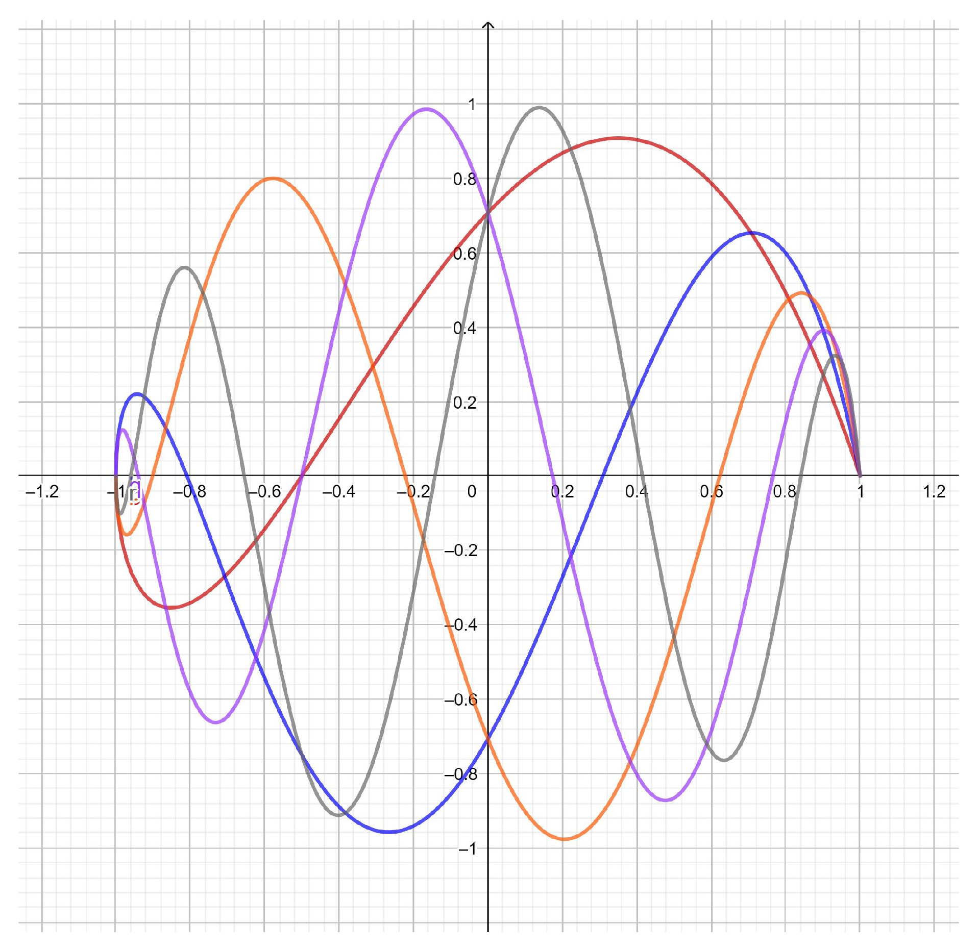
6. Orthogonality Properties

6.1. Orthogonality of the $T_{k+1/2}(x)$ and $U_{k+1/2}(x)$

In [2], the orthogonality properties of the first- and second-kind pseudo-Chebyshev functions of half-integer degree have been proven.

Theorem 3.

The first-kind pseudo-Chebyshev functions $T_{k+1/2}(x)$ verify the orthogonality property:

$${\int }_{-1}^1{T}_{h+\frac{1}{2}}(x)T_{k+\frac{1}{2}}(x)\frac{1}{\sqrt{1-x^2}}dx=0,(h\ne k),$$

(15)

where $h,k$ are integer numbers such that $h+k=2n$, $n=1,2,3,\dots$,

$${\int }_{-1}^1{T}_{k+\frac{1}{2}}^2(x)\frac{1}{\sqrt{1-x^2}}dx=\frac{\pi }{2}.$$

(16)

Proof of Theorem 3.

As a consequence of Werner formulas, we have:

$$\begin{array}{c}{\int }_{-1}^{1}cos\left[\left(h+\frac{1}{2}\right)arccos(x)\right]cos\left[\left(k+\frac{1}{2}\right)arccos(x)\right]\frac{1}{\sqrt{1-x^2}}dx=\\ =2{\int }_0^{\frac{\pi }{2}}cos[(2h+1)t]cos[(2k+1)t]dt=0,\end{array}$$

and:

$${\int }_{-1}^1{cos}^2\left[\left(k+\frac{1}{2}\right)arccos(x)\right]\frac{1}{\sqrt{1-x^2}}dx=2{\int }_0^{\frac{\pi }{2}}{cos}^2[(2k+1)t]dt=\frac{\pi }{2}.$$

(17)

 □

Theorem 4.

The second-kind pseudo-Chebyshev functions $U_{k+1/2}(x)$ verify the orthogonality property:

$${\int }_{-1}^1{U}_{h+\frac{1}{2}}(x)U_{k+\frac{1}{2}}(x)\sqrt{1-x^2}dx=0,(h\ne k),$$

(18)

where $h,k$ are integer numbers such that $h+k=2n$, $n=1,2,3,\dots$,

$${\int }_{-1}^1{U}_{k+\frac{1}{2}}^2(x)\sqrt{1-x^2}dx=\frac{\pi }{2}.$$

(19)

Proof of Theorem 4.

We have, under the above conditions:

$$\begin{array}{c}{\int }_{-1}^{1}sin\left[\left(h+\frac{1}{2}\right)arccos(x)\right]sin\left[\left(k+\frac{1}{2}\right)arccos(x)\right]\sqrt{1-x^2}dx=\\ =2{\int }_0^{\frac{\pi }{2}}sin[(2h+1)t]sin[(2k+1)t]dt=0,\end{array}$$

and:

$${\int }_{-1}^1{sin}^2\left[\left(k+\frac{1}{2}\right)arccos(x)\right]\sqrt{1-x^2}dx=2{\int }_0^{\frac{\pi }{2}}{sin}^2[(2h+1)t]dt=\frac{\pi }{2}.$$

(20)

 □

6.2. Orthogonality of the $V_{k+1/2}(x)$ and $W_{k+1/2}(x)$

The orthogonality properties of the third- and fourth-kind pseudo-Chebyshev functions are as follows:

Theorem 5.

The third-kind pseudo-Chebyshev functions $V_{k+1/2}(x)$ verify the orthogonality property:

$${\int }_{-1}^1{V}_{h+\frac{1}{2}}(x)V_{k+\frac{1}{2}}(x)\sqrt{1-x^2}dx=0,(h\ne k),$$

(21)

where $h,k$ are integer numbers such that $h+k=2n$, $n=1,2,3,\dots$,

$${\int }_{-1}^1{V}_{k+\frac{1}{2}}^2(x)\sqrt{1-x^2}dx=\frac{\pi }{2}.$$

(22)

Theorem 6.

The fourth-kind pseudo-Chebyshev functions $W_{k+1/2}(x)$ verify the orthogonality property:

$${\int }_{-1}^1{W}_{h+\frac{1}{2}}(x)W_{k+\frac{1}{2}}(x)\frac{1}{\sqrt{1-x^2}}dx=0,(h\ne k),$$

(23)

where $h,k$ are integer numbers such that $h+k=2n$, $n=1,2,3,\dots$,

$${\int }_{-1}^1{W}_{k+\frac{1}{2}}^2(x)\frac{1}{\sqrt{1-x^2}}dx=\frac{\pi }{2}.$$

(24)

7. Proofs of Equations (21) and (23)

• For the third-kind, using Definition (3) and recalling Equation (15), we find:

  $$\begin{array}{c}{\int }_{-1}^1{V}_{h+\frac{1}{2}}(x)V_{k+\frac{1}{2}}(x)\sqrt{1-x^2}dx={\int }_{-1}^1\frac{1}{1-x^2}{T}_{h+\frac{1}{2}}(x)T_{k+\frac{1}{2}}(x)\sqrt{1-x^2}dx=\\ ={\int }_{-1}^1{T}_{h+\frac{1}{2}}(x)T_{k+\frac{1}{2}}(x)\frac{1}{\sqrt{1-x^2}}dx=0,(h\ne k),\end{array}$$

  and by Equation (16):

  $${\int }_{-1}^1{V}_{k+\frac{1}{2}}^2(x)\sqrt{1-x^2}dx={\int }_{-1}^1{T}_{k+\frac{1}{2}}^2(x)\frac{1}{\sqrt{1-x^2}}dx=\frac{\pi }{2}.$$
• For the fourth-kind, using Definition (6) and recalling Equation (18), we find:

  $$\begin{array}{c}{\int }_{-1}^1{W}_{h+\frac{1}{2}}(x)W_{k+\frac{1}{2}}(x)\frac{1}{\sqrt{1-x^2}}dx={\int }_{-1}^1(1-x^2)U_{h-1}(x)U_{k-1}(x)\frac{1}{\sqrt{1-x^2}}dx=\\ ={\int }_{-1}^1{U}_{h-1}(x)U_{k-1}(x)\sqrt{1-x^2}dx=0,(h\ne k),\end{array}$$

  and by Equation (19):

  $$\begin{array}{c}\hfill \begin{array}{c}{\int }_{-1}^1{W}_{k+\frac{1}{2}}^2(x)\frac{1}{\sqrt{1-x^2}}dx={\int }_{-1}^1{U}_{k-\frac{1}{2}}^2(x)\sqrt{1-x^2}dx=\frac{\pi }{2}.\end{array}\end{array}$$

8. Representation of the Dirichlet Kernel

It is worth noting that the Dirichlet kernel $D_n(x)$ can be expressed in terms of pseudo-Chebyshev functions.

Theorem 7.

The representation formula of the Dirichlet kernel reads:

$$D_n(arccos(x))=W_n(x)=2T_{\frac{1}{2}}(x)U_{n-\frac{1}{2}}(x).$$

(25)

Proof of Theorem 7.

The Dirichlet kernel can be written as:

$$D_n(x)=\frac{sin\left[\left(n+\frac{1}{2}\right)x\right]}{sin\left(\frac{x}{2}\right)},$$

(26)

and therefore,

$$\begin{array}{c}{D}_n(arccos(x))=W_n(x)=\frac{sin\left[\left(n+\frac{1}{2}\right)arccos(x)\right]}{sin\left(\frac{arccos(x)}{2}\right)}=\sqrt{1-x^2}{U}_{n-\frac{1}{2}}(x)\sqrt{\frac{2}{1-x}}=\\ \sqrt{2(1+x)}{U}_{n-\frac{1}{2}}(x)=2T_{\frac{1}{2}}(x)U_{n-\frac{1}{2}}(x).\end{array}$$

 □

Summation of Trigonometric Series

A consequence of the preceding result is as follows. Consider a trigonometric series for an $L^1[-\pi ,\pi ]$, $2\pi$-periodic function f, that is,

$$f(x)\sim \frac{a_0}{2}+\sum _{k=1}^{\infty }{a}_{k}cos(kx)+b_{k}sin(kx),$$

(27)

where $a_k$ and $b_k$ are the Fourier coefficients of f.

By Carleson’s theorem [19], the above series converges, in the mean and even pointwise, to a set of a Lebesgue measure zero.

Since the partial sums of the above series are written:

$$s_n(x,f)=\frac{a_0}{2}+\sum _{k=1}^n{a}_{k}cos(kx)+b_{k}sin(kx)=\frac{1}{2\pi }{\int }_{-\pi }^{\pi }f(x-t)D_n(t)dt,$$

(28)

the following result holds true:

Theorem 8.

The partial sums of a Fourier series can be written in terms of the pseudo-Chebyshev functions as follows:

$$\begin{array}{c}{s}_n(x,f)=\frac{1}{\pi }{\int }_{-1}^{1}f(x-arccos(\tau ))W_n(\tau )\frac{1}{\sqrt{1-{\tau }^2}}d\tau =\\ =\frac{2}{\pi }{\int }_{-1}^{1}f(x-arccos(\tau ))T_{\frac{1}{2}}(\tau )U_{n-\frac{1}{2}}(\tau )\frac{1}{\sqrt{1-{\tau }^2}}d\tau =\\ =\frac{1}{\pi }{\int }_{-1}^{1}f(x-arccos(\tau ))\frac{U_{n-\frac{1}{2}}(\tau )}{U_{\frac{1}{2}}(\tau )}d\tau .\end{array}$$

9. Conclusions

We have shown that the family of pseudo-Chebyshev function recently introduced in [1,2] can be enlarged by introducing the half-integer degree pseudo-Chebyshev functions of the third and fourth kind, satisfying the orthogonality property with respect to the classical weights of the second and first-kind Chebyshev polynomials.

Since the pseudo-Chebyshev functions arise from the Grandi (rhodonea) curves, assuming a fractional index [1], many other possible pseudo-Chebyshev functions could be considered. For example, we have by definition:

$$T_{\frac{m}{n}}(x)=cos\left[\frac{m}{n}arccosx\right],$$

(29)

and:

$$\sqrt{1-x^2}{U}_{\frac{m}{n}-1}(x)=sin\left[\frac{m}{n}arccosx\right].$$

(30)

Setting:

$$\frac{m}{n}=\frac{p}{q}+\frac{r}{s},$$

(31)

and using the cosine addition formulas, we find the recursion:

$$T_{\frac{m}{n}}(x)=T_{\frac{p}{q}}(x)T_{\frac{r}{s}}(x)-(1-x^2)U_{\frac{p}{q}-1}(x)U_{\frac{r}{s}-1}(x),$$

(32)

and by the sine addition formulas,

$$U_{\frac{m}{n}}(x)=U_{\frac{p}{q}-1}(x)T_{\frac{r}{s}}(x)+U_{\frac{r}{s}}(x)T_{\frac{p}{q}}(x).$$

(33)

We have shown that the particular case when $\frac{m}{n}=k+\frac{1}{2}$ produces functions that are orthogonal in the basic interval $(-1,1)$ with respect to known weights, but we cannot exclude that other choices exist of rational indices (corresponding to different Grandi curves) producing sequences of functions that verify the properties of some interest. This is an open problem, which could be solved in the near future. Finally, it is important to note the powerful tool represented by Chebyshev polynomials; in fact, these polynomials can be used in many important and various fields and in particular to simplify the properties of other families of polynomials, for instance in the description of Bernoulli and Lucas polynomials [20,21].

References

1. Ricci, P.E. Complex spirals and pseudo-Chebyshev polynomials of fractional degree. Symmetry 2018, 10, 671. [Google Scholar] [CrossRef]
2. Brandi, P.; Ricci, P.E. Some properties of the pseudo-Chebyshev polynomials of half-integer degree. J. Class. Anal. 2019. submitted. [Google Scholar]
3. Mason, J.C.; Handscomb, D.C. Chebyshev Polynomials; Chapman and Hall: New York, NY, USA; CRC: Boca Raton, FL, USA, 2003. [Google Scholar]
4. Rivlin, T.J. The Chebyshev Polynomials; J. Wiley and Sons: New York, NY, USA, 1974. [Google Scholar]
5. Ricci, P.E. Alcune osservazioni sulle potenze delle matrici del secondo ordine e sui polinomi di Tchebycheff di seconda specie, Atti Accad. Sci. Torino 1975, 109, 405–410. [Google Scholar]
6. Ricci, P.E. Sulle potenze di una matrice. Rend. Mater. 1976, 9, 179–194. [Google Scholar]
7. Ricci, P.E. Una proprietà iterativa dei polinomi di Chebyshev di prima specie in più variabili. Rend. Mater. Appl. 1986, 6, 555–563. [Google Scholar]
8. Boyd, J.P. Chebyshev and Fourier Spectral Methods, 2nd ed.; Dover: Mineola, NY, USA, 2001. [Google Scholar]
9. Cesarano, C. Identities and generating functions on Chebyshev polynomials. Georgian Math. J. 2012, 19, 427–440. [Google Scholar] [CrossRef]
10. Cesarano, C. Integral representations and new generating functions of Chebyshev polynomials. Hacet. J. Math. Stat. 2015, 44, 535–546. [Google Scholar] [CrossRef]
11. Cesarano, C.; Cennamo, G.M.; Placidi, L. Operational methods for Hermite polynomials with applications. WSEAS Trans. Math. 2014, 13, 925–931. [Google Scholar]
12. Cesarano, C. Generalized Chebyshev polynomials. Hacet. J. Math. Stat. 2014, 43, 731–740. [Google Scholar]
13. Cesarano, C.; Fornaro, C. Operational identities on generalirized two-variable Chebyshev polynomials. Int. J. Pure Appl. Math. 2015, 100, 59–74. [Google Scholar] [CrossRef]
14. Cesarano, C.; Fornaro, C. A note on two-variable Chebyshev polynomials. Georgian Math. J. 2017, 24, 339–349. [Google Scholar] [CrossRef]
15. Srivastava, H.M.; Ricci, P.E.; Natalini, P. A Family of Complex Appell Polynomial Sets. Real Acad. Sci. Exact. Fis Nat. Ser. A Math. 2018. to appear. [Google Scholar] [CrossRef]
16. Aghigh, K.; Masjed-Jamei, M.; Dehghan, M. A survey on third and fourth kind of Chebyshev polynomials and their applications. Appl. Math. Comput. 2008, 199, 2–12. [Google Scholar] [CrossRef]
17. Doha, E.H.; Abd-Elhameed, W.M.; Alsuyuti, M.M. On using third and fourth kinds Chebyshev polynomials for solving the integrated forms of high odd-order linear boundary value problems. J. Egypt. Math. Soc. 2014. to appear. [Google Scholar] [CrossRef]
18. Kim, T.; Kim, D.S.; Dolgy, D.V.; Kwon, J. Sums of finite products of Chebyshev polynomials of the third and fourth kinds. Adv. Differ. Equ. 2018, 2018, 283. [Google Scholar] [CrossRef]
19. Carleson, L. On convergence and growth of partial sums of Fourier series. Acta Math. 1966, 116, 135–157. [Google Scholar] [CrossRef]
20. Kim, D.S.; Kim, T.; Lee, S.H. Some identities for Bernoulli polynomials involving Chebyshev polynomials. J. Comput. Anal. Appl. 2014, 16, 172–180. [Google Scholar]
21. Kim, T.; Kim, D.S.; Dolgy, D.V.; Kwon, J. Representing sums of finite products of Chebyshev polynomials of the first kind and Lucas polynomials by Chebyshev polynomials. Mathematics 2019, 7, 26. [Google Scholar] [CrossRef]
Figure 1. Pseudo T k + 1 / 2 , k = 1 , 2 , 3 , 4 , 5 . 1, green; 2, red; 3, blue; 4, orange.
Mathematics 07 00180 g001
Figure 2. Pseudo U k + 1 / 2 , k = 1 , 2 , 3 , 4 , 5 . 1, green; 2, red; 3, blue; 4, orange.
Mathematics 07 00180 g002
Figure 3. V k ( x ) , k = 1 , 2 , 3 , 4 , 5 . 1, green; 2, red; 3, blue; 4, orange; 5, violet.
Mathematics 07 00180 g003
Figure 4. W k ( x ) , k = 1 , 2 , 3 , 4 , 5 . 1, green; 2, red; 3, blue; 4, orange; 5, violet.
Mathematics 07 00180 g004
Figure 5. V k + 1 / 2 , k = 1 , 2 , 3 , 4 , 5 . 1, grey; 2, red; 3, blue; 4, orange; 5, violet.
Mathematics 07 00180 g005
Figure 6. W k + 1 / 2 , k = 1 , 2 , 3 , 4 , 5 . 1, red; 2, blue; 3, orange; 4, violet; 5, grey.
Mathematics 07 00180 g006