Abstract
Existing fuzzy analytic hierarchy process (FAHP) methods usually aggregate the fuzzy pairwise comparison results produced by multiple decision-makers (DMs) rather than the fuzzy weights estimations. This is problematic because fuzzy pairwise comparison results are subject to uncertainty and lack consensus. To address this problem, a partial-consensus posterior-aggregation FAHP (PCPA-FAHP) approach is proposed in this study. The PCPA-FAHP approach seeks a partial consensus among most DMs instead of an overall consensus among all DMs, thereby increasing the possibility of reaching a consensus. Subsequently, the aggregation result is defuzzified using the prevalent center-of-gravity method. The PCPA-FAHP approach was applied to a supplier selection problem to validate its effectiveness. According to the experimental results, the PCPA-FAHP approach not only successfully found out the partial consensus among the DMs, but also shrunk the widths of the estimated fuzzy weights to enhance the precision of the FAHP analysis.
1. Introduction
Analytic hierarchy process (AHP) has been widely applied to multi-criteria decision-making problems in various fields [1,2,3]. However, AHP is based on pairwise comparison results that are subjective. To solve this problem, AHP usually aggregates the pairwise comparison results by multiple decision-makers (DMs) [4,5,6]. In most past studies, the number of DMs ranged from 3 [7,8] to up to 30 [9]. In addition, a DM may be uncertain whether the pairwise comparison results are reflective of his/her beliefs or not. To consider such uncertainty, pairwise comparison results can be mapped to fuzzy values. The two treatments give rise to the prevalent multi-DM fuzzy AHP (FAHP) methods.
According to Forman and Peniwati [10], there are two ways to aggregate multiple DMs’ judgments in FAHP. The first way, the aggregating individual judgements (AIJ) way, aggregates the pairwise comparison results. The other way, the aggregating individual priorities (AIP) way, aggregates the estimated fuzzy weights/priorities. The AIJ way is an anterior aggregation, while the AIP way is a posterior aggregation. The AIJ way considerably simplifies the required computation because the fuzzy weights are estimated just once, and therefore is more prevalent [11]. However, since pairwise comparison results are subjective and uncertain, the AIP way is problematic. In contrast, few studies have implemented AIP-type FAHP methods. Pan [12] proposed an FAHP approach in which each DM solved an individual FAHP problem using the fuzzy geometric mean (FGM) method. Then, the fuzzy weights estimated by the DMs were aggregated using the max-min operator, i.e., fuzzy intersection (FI) or the minimum T-norm. After that, the aggregation result was defuzzified using the center-of-gravity (COG) method [13]. The same operator has been widely adopted to measure the consensus among multiple DMs [14,15]. A different aggregation mechanism was proposed by [16,17] that minimized the sum of the squared deviations between each DM’s judgement and the aggregation result. However, the aggregation mechanism assumed the existence of consensus, and derived the aggregation result directly. It was possible that the values of a fuzzy weight estimated by the DMs were very different, i.e., the values did not contain each other. Pan’s method did not address this issue. To address this issue, several attempts have been made in the past. For example, Chen [18] proposed the concept of partial consensus that sought for a consensus among some of the DMs rather than all DMs. The method was applied to the problem of forecasting the foreign exchange rate in [19]. Recently, Chen [20] evaluated the entropy of the FI result. If the entropy was above a threshold, then the consensus was insufficient, and the DMs needed to modify their forecasts. However, these attempts were made for fuzzy collaborative forecasting or design rather than for FAHP. A fuzzy collaborative forecasting problem is usually a supervised learning problem; there are actual values. However, there are no actual values of fuzzy weights in an FAHP problem.
To address the problem of Pan’s FAHP method, in this study, a partial-consensus posterior-aggregation FAHP (PCPA-FAHP) method is proposed. In the proposed PCPA-FAHP approach, each DM applies the prevalent FGM approach to estimate the fuzzy weights. Then, the partial-consensus FI (PCFI) method [18] is applied to aggregate the estimation results, so as to derive the narrowest range of the fuzzy weight. The PCFI method finds out the partial consensus among most DMs instead of the overall consensus among all DMs. The former is obviously easier than the latter. After that, the COG method is applied to defuzzify the aggregation results, generating a crisp/representative value. Compared to the existing methods, the proposed PCPA-FAHP approach has the following novel characteristics:
- (1)
- The proposed PCPA-FAHP approach adopts a posterior aggregation. Namely, the fuzzy weights estimated by the DMs, rather than the fuzzy pairwise comparison results by them, are aggregated: A multiple-DM FAHP method can be considered as a fuzzy collaborative forecasting (FCF) approach. Most existing FCF approaches adopt a posterior aggregation, i.e., the forecasts by multiple DMs, rather than their opinions, are aggregated [21,22]. If the forecasting performance based on the aggregation result is not satisfactory, the DMs modify their opinions by referring to others’ opinions [23,24]. However, existing FCF methods belong to supervised learning methods, while the PCPA-FAHP approach does not because there is no actual value of the fuzzy weight. In addition, it is not easy for the DMs to modify their pairwise comparison results by referring to others’ because the relative importance levels of factors/attributes/criteria are correlated and cannot be modified in an independent way.
- (2)
- When a consensus among all DMs cannot be achieved, the partial consensus, i.e., the consensus among most DMs, is to be sought.
The remainder of this paper is organized as follows. Section 2 introduces the PCPA-FAHP approach. A real case is used in Section 3 to illustrate the applicability of the PCPA-FAHP approach. Some existing methods are also applied to the case for a comparison in Section 4. Section 5 concludes this study. Some possible topics are also provided for further investigation.
2. The Proposed Methodology
The PCPA-FAHP approach is proposed in this study for comparing the relative importance levels or priorities of several factors/attributes-criteria. The PCPA-FAHP approach consists of the following steps:
- Step 1.
- Each DM applies the FGM approach to estimate the fuzzy weights.
- Step 2.
- Apply FI to aggregate the estimation results, so as to derive the narrowest range of each fuzzy weight.
- Step 3.
- If the overall consensus among the DMs does not exist, go to Step 4; otherwise, go to Step 5.
- Step 4.
- Apply PCFI to aggregate the estimation results, so as to derive the narrowest range of each fuzzy weight.
- Step 5.
- Apply COG to defuzzify the aggregation result, so as to generate a crisp/representative value.
The procedure of the PCPA-FAHP approach is illustrated with a flowchart in Figure 1.
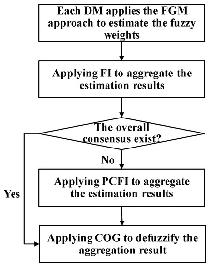
Figure 1.
The procedure of the partial-consensus posterior-aggregation fuzzy analytic hierarchy process (PCPA-FAHP) approach.
2.1. Applying the FGM Approach to Estimate the Fuzzy Weights
In the FGM approach, at first each DM expresses his/her opinion on the relative importance/priority of a factor/attribute/criterion over that of another with linguistic terms such as “as equal as”, “weakly more important than”, “strongly more important than”, “very strongly more important than”, and “absolutely more important than”. Without loss of generality, these linguistic terms can be mapped to triangular fuzzy numbers (TFNs) such as:
- L1:
- “As equal as” = (1, 1, 3);
- L2:
- “Weakly more important than” = (1, 3, 5);
- L3:
- “Strongly more important than” = (3, 5, 7);
- L4:
- “Very strongly more important than” = (5, 7, 9);
- L5:
- “Absolutely more important than” = (7, 9, 9);
which are illustrated in Figure 2. It is a theoretically challenging task to find a set of TFNs for the linguistic terms to increase the possibility of reaching a consensus.
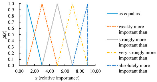
Figure 2.
The triangular fuzzy numbers (TFNs) for the linguistic terms.
Based on the pairwise comparison results by the m-th DM, a fuzzy pairwise comparison matrix is constructed as:
where
is the fuzzy pairwise comparison result embodying the relative importance of factor/attribute/criterion i over factor/attribute/criterion j. is chosen from the linguistic terms in Figure 2. is a positive comparison if . The fuzzy eigenvalue and eigenvector of , indicated respectively with and , satisfy
and
where (−) and (×) denote fuzzy subtraction and multiplication, respectively. The fuzzy maximal eigenvalue and weight of each criterion are derived respectively as
Based on , the consistency among the fuzzy pairwise comparison results is evaluated as
where R.I. is the random index [25]. The fuzzy pairwise comparison results are inconsistent if or [25], which can be relaxed to or if the matrix size is large [26,27].
The FGM method estimates the values of fuzzy weights as
Based on (9), the fuzzy maximal eigenvalue can be estimated as
Obviously, Equations (9) and (10) are fuzzy weighted average (FWA) problems. A variant of FGM (a simplified yet more prevalent version), indicated with FGMi, is to ignore the dependency between the dividend and divisor of either equation.
2.2. FI for Finding out the Overall Consensus
As mentioned previously, a multi-DM post-aggregation FAHP problem is analogous to an unsupervised FCF problem to which a suitable consensus aggregator is critical. According to Kuncheva and Krishnapuram [28], a consensus aggregator should meet three requirements: Symmetry, selective monotonicity, and unanimity. They proposed three aggregation rules: The minimum aggregation rule, the maximum aggregation rule, and the average aggregation rule, for which the degree of consensus was measured in terms of the highest discrepancy. FI is the most prevalent consensus aggregator in FCF methods [24,29]. FI finds out the values common to those estimated by all DMs. Therefore, it can be used to find out the overall consensus among the DMs.
When the fuzzy weight estimated by each DM is approximated with a TFN, the FI result will be a polygon-shaped fuzzy number (see Figure 3) [29] that embodies the DMs’ overall consensus of the weight/priority of the factor/attribute/criterion:
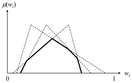
Figure 3.
The fuzzy intersection (FI) result.
However, it is possible that the FI result is an empty set, which means there is no overall consensus among the DMs.
2.3. PCFI for Finding out the Partial Consensus
When there is no overall consensus among all DMs, the partial consensus among them, i.e., the consensus among most DMs, can be sought instead.
Definition 1.
(PCFI) [20] The H/M PCFI of the i-th fuzzy weight estimated by the M DMs, i.e., ~ is indicated with such that
where g() ∈ Z+; 1 ≤ g() ≤ M; g(p) ∩ g(q) = ∅ ∀ p ≠ q; H ≥ 2.
For example, the 2/3 PCFI of ~ can be obtained as
which is illustrated in Figure 4.
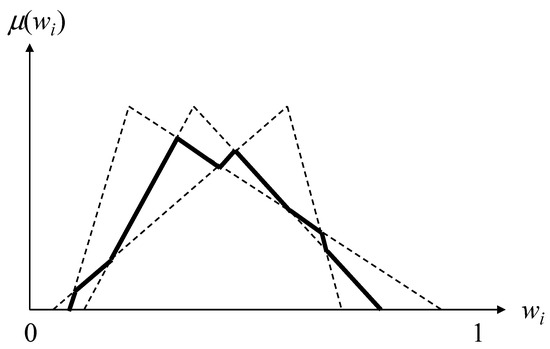
Figure 4.
The 2/3 partial consensus fuzzy intersection (PCFI) result.
The PCFI aggregator meets four requirements: Boundary, monotonicity, commutativity, and associativity. In addition, the following properties hold for the H/M PCFI result:
- (1)
- FI is equivalent to M/M PCFI.
- (2)
- H − 1 membership functions are outside the H/M PCFI result. In contrast, M − 1 membership functions are outside the FI result.
- (3)
- The range of is wider than that of if H1 < H2.
- (4)
- The range of any PCFI result is obviously wider than that of the FI result.
- (5)
- For the training data, every PCFI result contains the actual values [20].
- (6)
- For the testing data, the probability that actual values are contained is higher in a PCFI result than in the FI result [20].
The PCFI result is also a polygon-shaped fuzzy number (see Figure 4). Compared with the original TFNs, the PCFI result has a narrower range while still containing the actual value. Therefore, the precision of estimating the fuzzy weight will be improved after applying the PCFI. In addition, it is possible to find partial consensus among the DMs using the PCFI even if there is no overall consensus when the FI is applied.
2.4. COG for Defuzzifying the Aggregation Result
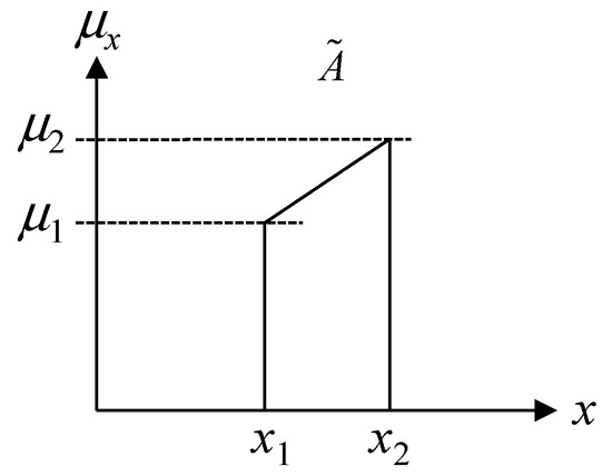
The PCFI result in Figure 4 can be represented as the union of several non-normal trapezoidal fuzzy numbers (TrFNs) (see Figure 5):
where is the r-th endpoint of ; . For any x value,
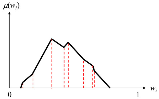
Figure 5.
The PCFI result as a union of non-normal trapezoidal fuzzy numbers (TrFNs).
COG is applied to defuzzify :
to which the following theorems are helpful.
Theorem 1.
Let be a non-normal TrFN as shown in Figure 6. Then the integral of is
Figure 6.
A non-normal TrFN.
Proof.
Theorem 1 is proved. □
Theorem 2.
Let be a non-normal TrFN as shown in Figure 6. Then the integral of is
Proof.
Theorem 2 is proved. □
3. Application to a Supplier Selection Problem
The supplier selection problem discussed in Lima Junior et al. [7] was used to illustrate the applicability of the proposed methodology. In the supplier selection problem, the performance of a supplier was assessed along five dimensions including quality, price, delivery, supplier profile, and supplier relationship. To aggregate the performances along the five dimensions, fuzzy weighted average (FWA) was applicable, for which the weight of each dimension needed to be specified. To this end, the PCFI-FAHP approach was applied.
Three DMs, including one industrial engineering manager, one production control manager, and one procurement department manager, were involved in the supplier selection problem. At first, each of them utilized the following linguistic terms [30] to express his/her belief about the relative importance of a dimension over another:
- L1:
- “As equal as” = (1, 1, 3);
- L2:
- “Weakly more important than” = (1, 3, 5);
- L3:
- “Strongly more important than” = (3, 5, 7);
- L4:
- “Very strongly more important than” = (5, 7, 9);
- L5:
- “Absolutely more important than” = (7, 9, 9).
Based on these inputs, the fuzzy pairwise comparison matrixes were constructed for the DMs in Table 1.

Table 1.
The fuzzy pairwise comparison matrixes constructed for the decision-makers (DMs).
Each DM applied FGM to estimate the fuzzy maximal eigenvalue and fuzzy weights from the corresponding fuzzy pairwise comparison matrix. As a result, the estimated fuzzy maximal eigenvalues were:
- ,
- ,
- .
The corresponding consistency indexes were
- = ,
- = ,
- = ,
showing certain levels of consistency since ~ ≤ 0.3. In addition, the estimated fuzzy weights are summarized in Figure 7.
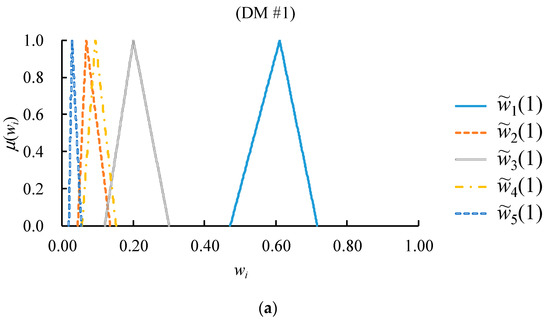
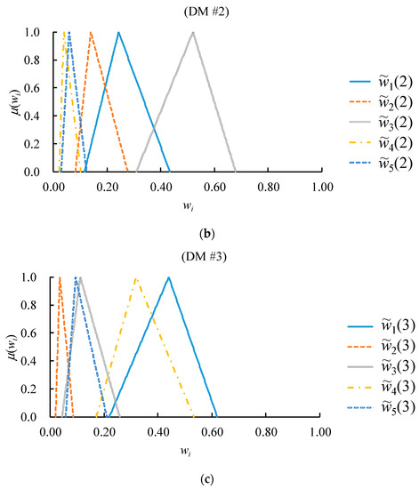
Figure 7.
The estimated fuzzy weights: (a) by DM #1; (b) by DM #2; (c) by DM #3.
Subsequently, FI was applied to aggregate the fuzzy weights estimated by the DMs. However, unfortunately the overall consensus did not exist. For example, the result of aggregating the values of estimated by the DMs is illustrated in Figure 8. The FI result was an empty set, showing a lack of (overall) consensus. In addition, overall consensus was not achieved for the values of , , or .
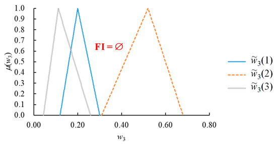
Figure 8.
The FI result.
As a consequence, the partial consensus, rather than the overall consensus, was sought. It is noteworthy that there were only two levels of PCFI in the supplier selection problem, 2/3 PCFI and 3/3 PCFI. Between them, 3/3 PCFI was equal to FI. The result of applying 2/3 PCFI to the values of estimated by the DMs is shown in Figure 9. There existed some partial consensus among the DMs. In addition, the DMs also achieved some partial consensus concerning the values of the other fuzzy weights.
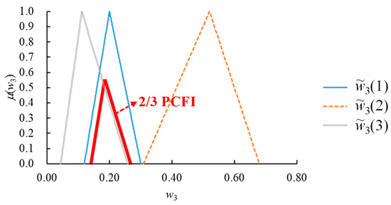
Figure 9.
The result of applying 2/3 PCFI to the values of estimated by the DMs.
Based on the PCFI results, the minimums, maximums, and widths of the fuzzy weights are summarized in Table 2. The minimal and average widths were 0.054 and 0.401, respectively.
Table 2.
The minimums, maximums, and range widths of the fuzzy weights.
COG was applied to defuzzify the fuzzy weights. The results are shown in Table 3.
Table 3.
The defuzzification results.
However, the sum of the defuzzified weights might not be 1 anymore, which required a re-normalization. The results are shown in Table 4.
Table 4.
The re-normalization results.
4. A Comparison with Some Existing Methods
To make a comparison, in this section four existing methods including FGM [31], FGMi [32], fuzzy extent analysis (FEA) [33], and FEAi [8,11,30] were also applied to the supplier selection problem:
- (1)
- The results obtained using FGM and FGMi were fuzzy, while those obtained using FEA and FEAi were crisp.
- (2)
- All the existing methods assumed there was consensus among the DMs.
In the FGM method, the fuzzy pairwise comparison results by the DMs were aggregated using FGM. Then, the fuzzy maximal eigenvalue and fuzzy weights were estimated from the aggregation result using FGM as well. The FGMi method was basically identical to the FGM method, except for the simplification of calculation by ignoring the dependence between the dividend and divisor. In both methods, COG was applied to defuzzify the fuzzy weights. A re-normalization was also required after defuzzification.
In the FEA method, the fuzzy pairwise comparison results by the DMs were also aggregated using FGM. Then, the fuzzy synthetic extent of each criterion was derived using fuzzy arithmetic mean. The weight of the criterion was set to its minimal degree of being the maximum. The only difference between the FEAi method and the FEA method is the ignorance of the dependence between the dividend and divisor. In both methods, defuzzification and re-normalization were not necessary.
The results obtained using the existing methods are summarized in Table 5. However, it was not possible to say which method was the most accurate method, since there was no actual value of a weight. Nevertheless, the weights obtained using the FGM were the closest to those obtained using the proposed methodology. In contrast, the weights obtained using the FEAi method were the farthest.
Table 5.
The weights estimated using various methods.
The average widths of the fuzzy weights obtained using various methods were compared and the results are shown in Figure 10. Obviously, the proposed methodology achieved the highest precision by minimizing the average width of the fuzzy weights, which was obviously due to the fuzzy collaboration mechanism.

Figure 10.
The average widths of the fuzzy weights estimated using various methods.
Compared to the existing FAHP methods, the proposed methodology was distinctive in that it excluded DM opinions that could not be included in the consensus. The proposed methodology did not attempt to compromise opposing DM opinions into neutral results. A DM whose opinion was excluded either accepted the consensus or modified his/her opinion to be included. In other words, it was important for DMs to reach consensus before aggregating their opinions. In addition, the overlap among the fuzzy weights estimated by the DMs seemed to be a very good tool for the visualization of consensus.
5. Conclusions
Among existing multi-DM FAHP methods, most of them aggregate the fuzzy pairwise comparison results by the DMs before deriving (or estimating) the fuzzy maximal eigenvalue and fuzzy weights. This is problematic because the fuzzy pairwise comparison results are uncertain and inconsistent. Instead, aggregating the fuzzy weights by the DMs, which are compromised results, in a posterior way seems to be more reasonable. However, a problem facing such a way is that there may be no consensus among the DMs, i.e., there was no intersection among the fuzzy weights specified by them. One way to address this problem is to seek the partial consensus among most DMs instead of the overall consensus among all DMs. From this point of view, the PCPA-FAHP approach is proposed in this study.
The PCPA-FAHP approach was applied to a supplier selection problem to validate its effectiveness. Some existing methods were also applied to the supplier selection problem to make a comparison. According to the experimental results:
- (1)
- Among the methods compared in the supplier selection problem, only the PCPA-FAHP approach was able to check the existence of the consensus among the DMs.
- (2)
- Although there was no overall consensus among all DMs in the supplier selection problem, some partial consensus did exist among most DMs.
- (3)
- The fuzzy collaboration mechanism employed in the PCPA-FAHP approach successfully shrunk the widths of the estimated fuzzy weights, thereby enhancing the precision of the FAHP analysis.
- (4)
- Among existing methods, the results obtained using FGM were the closest to those obtained using the PCPA-FAHP approach. However, the estimation precision achieved using FGM was much worse than that achieved using the PCPA-FAHP approach.
The PCPA-FAHP method needs to be applied to more real cases to further elaborate its effectiveness. In addition, more advanced collaboration mechanisms can be designed in future studies to further enhance the estimation precision. Furthermore, the uncertain pairwise comparison results can be expressed with rough numbers instead of fuzzy numbers [15,16], which constitutes a rough AHP (RAHP) problem [34]. The proposed methodology should be extended to deal with such problems.
Author Contributions
All authors contributed equally to the writing of this paper. All authors read and approved the final manuscript. Writing original draft, T.-C.T.C. and Y.-C.W.; Writing review & editing, T.-C.T.C. and Y.-C.W.
Funding
This research received no external funding.
Acknowledgments
We are thankful to the referees for their careful reading of the manuscript and for valuable comments and suggestions that greatly improved the presentation of this work.
Conflicts of Interest
The authors declare that there is no conflict of interest regarding the publication of this article.
References
- Van Laarhoven, P.J.M.; Pedrycz, W. A fuzzy extension of Saaty’s priority theory. Fuzzy Sets Syst. 1983, 11, 229–241. [Google Scholar] [CrossRef]
- Promentilla, M.A.B.; Furuichi, T.; Ishii, K.; Tanikawa, N. A fuzzy analytic network process for multi-criteria evaluation of contaminated site remedial countermeasures. J. Environ. Manag. 2008, 88, 479–495. [Google Scholar] [CrossRef] [PubMed]
- Jain, V.; Sakhuja, S.; Thoduka, N.; Aggarwal, R.; Sangaiah, A.K. Supplier selection using fuzzy AHP and TOPSIS: a case study in the Indian automotive industry. Neural Comput. Appl. 2016, 29, 555–564. [Google Scholar] [CrossRef]
- Kahraman, C.; Cebeci, U.; Ruan, D. Multi-attribute comparison of catering service companies using fuzzy AHP: The case of Turkey. Int. J. Prod. Econ. 2004, 87, 171–184. [Google Scholar] [CrossRef]
- Ignatius, J.; Hatami-Marbini, A.; Rahman, A.; Dhamotharan, L.; Khoshnevis, P. A fuzzy decision support system for credit scoring. Neural Comput. Appl. 2016, 29, 921–937. [Google Scholar] [CrossRef]
- Foroozesh, N.; Tavakkoli-Moghaddam, R.; Mousavi, S.M. A novel group decision model based on mean–variance–skewness concepts and interval-valued fuzzy sets for a selection problem of the sustainable warehouse location under uncertainty. Neural Comput. Appl. 2017, 30, 3277–3293. [Google Scholar] [CrossRef]
- Junior, F.R.L.; Osiro, L.; Carpinetti, L.C.R. A comparison between Fuzzy AHP and Fuzzy TOPSIS methods to supplier selection. Appl. Soft Comput. 2014, 21, 194–209. [Google Scholar] [CrossRef]
- Güran, A.; Uysal, M.; Ekinci, Y. An additive FAHP based sentence score function for text summarization. ITC 2017, 46, 53–69. [Google Scholar] [CrossRef]
- Gnanavelbabu, A.; Arunagiri, P. Ranking of MUDA using AHP and Fuzzy AHP algorithm. Mater. Today: Proc. 2018, 5, 13406–13412. [Google Scholar] [CrossRef]
- Forman, E.; Peniwati, K. Aggregating individual judgments and priorities with the analytic hierarchy process. Eur. J. Oper. Res. 1998, 108, 165–169. [Google Scholar] [CrossRef]
- Wang, Y.-C.; Chen, T.; Yeh, Y.-L. Advanced 3D printing technologies for the aircraft industry: a fuzzy systematic approach for assessing the critical factors. Int. J. Adv. Manuf. Technol. 2018, 1–11. [Google Scholar] [CrossRef]
- Pan, N.-F. Fuzzy AHP approach for selecting the suitable bridge construction method. Autom. Constr. 2008, 17, 958–965. [Google Scholar] [CrossRef]
- Hanss, M. Applied Fuzzy Arithmetic; Springer: Berlin/Heidelberg, Germany, 2005. [Google Scholar]
- Ostrosi, E.; Haxhiaj, L.; Fukuda, S. Fuzzy modelling of consensus during design conflict resolution. Res. Eng. Design 2011, 23, 53–70. [Google Scholar] [CrossRef]
- Chen, T. Forecasting the Unit Cost of a Product with Some Linear Fuzzy Collaborative Forecasting Models. Algorithms 2012, 5, 449–468. [Google Scholar] [CrossRef]
- Ostrosi, E.; Bluntzer, J.-B.; Zhang, Z.; Stjepandić, J. Car style-holon recognition in computer-aided design. J. Comput. Design Eng. 2018. [Google Scholar] [CrossRef]
- Zhang, Z.; Xu, D.; Ostrosi, E.; Yu, L.; Fan, B. A systematic decision-making method for evaluating design alternatives of product service system based on variable precision rough set. J. Intell. Manuf. 2017. [Google Scholar] [CrossRef]
- Chen, T. A hybrid fuzzy and neural approach with virtual experts and partial consensus for DRAM price forecasting. Int. J. Innov. Comput. Infor. Control 2012, 8, 583–597. [Google Scholar]
- Chen, T. Foreign exchange rate forecasting with a virtual-expert partial-consensus fuzzy-neural approach for semiconductor manufacturers in Taiwan. IJISE 2013, 13, 73–91. [Google Scholar] [CrossRef]
- Chen, T. Estimating unit cost using agent-based fuzzy collaborative intelligence approach with entropy-consensus. Appl. Soft Comput. 2018, 73, 884–897. [Google Scholar] [CrossRef]
- Mitra, S.; Banka, H.; Pedrycz, W. Rough–Fuzzy Collaborative Clustering. IEEE Trans. Syst. Man Cybern. B Cybern. 2006, 36, 795–805. [Google Scholar] [CrossRef]
- Chen, T.; Romanowski, R. Forecasting the productivity of a virtual enterprise by agent-based fuzzy collaborative intelligence—With Facebook as an example. Appl. Soft Comput. 2014, 24, 511–521. [Google Scholar] [CrossRef]
- Pedrycz, W.; Rai, P. Collaborative clustering with the use of Fuzzy C-Means and its quantification. Fuzzy Sets Syst. 2008, 159, 2399–2427. [Google Scholar] [CrossRef]
- Chen, T.; Wang, Y.-C. An Agent-Based Fuzzy Collaborative Intelligence Approach for Precise and Accurate Semiconductor Yield Forecasting. IEEE Trans. Fuzzy Syst. 2014, 22, 201–211. [Google Scholar] [CrossRef]
- Saaty, T.L. The Analytic Hierarchy Process; McGraw-Hill Education: New York, NY, USA, 1980. [Google Scholar]
- Wedley, W.C. Consistency prediction for incomplete AHP matrices. Math. Comput. Model. 1993, 17, 151–161. [Google Scholar] [CrossRef]
- Klaus, D. Goepel Business Performance Management Singapore. Available online: https://bpmsg.com/2013/12/ (accessed on 20 October 2018).
- Kuncheva, L.I.; Krishnapuram, R. A fuzzy consensus aggregation operator. Fuzzy Sets Syst. 1996, 79, 347–356. [Google Scholar] [CrossRef]
- Chen, T.; Lin, Y.-C. A fuzzy-neural system incorporating unequally important expert opinions for semiconductor yield forecasting. Int. J. Unc. Fuzzy Knowl. Syst. 2008, 16, 35–58. [Google Scholar] [CrossRef]
- Zyoud, S.H.; Kaufmann, L.G.; Shaheen, H.; Samhan, S.; Fuchs-Hanusch, D. A framework for water loss management in developing countries under fuzzy environment: Integration of Fuzzy AHP with Fuzzy TOPSIS. Expert Syst. Appl. 2016, 61, 86–105. [Google Scholar] [CrossRef]
- Buckley, J.J. Fuzzy hierarchical analysis. Fuzzy Sets Syst. 1985, 17, 233–247. [Google Scholar] [CrossRef]
- Zheng, G.; Zhu, N.; Tian, Z.; Chen, Y.; Sun, B. Application of a trapezoidal fuzzy AHP method for work safety evaluation and early warning rating of hot and humid environments. Saf. Sci. 2012, 50, 228–239. [Google Scholar] [CrossRef]
- Chang, D.-Y. Applications of the extent analysis method on fuzzy AHP. Eur. J. Oper. Res. 1996, 95, 649–655. [Google Scholar] [CrossRef]
- Aydogan, E.K. Performance measurement model for Turkish aviation firms using the rough-AHP and TOPSIS methods under fuzzy environment. Expert Syst. Appl. 2011, 38, 3992–3998. [Google Scholar] [CrossRef]
© 2019 by the authors. Licensee MDPI, Basel, Switzerland. This article is an open access article distributed under the terms and conditions of the Creative Commons Attribution (CC BY) license (http://creativecommons.org/licenses/by/4.0/).