All articles published by MDPI are made immediately available worldwide under an open access license. No special
permission is required to reuse all or part of the article published by MDPI, including figures and tables. For
articles published under an open access Creative Common CC BY license, any part of the article may be reused without
permission provided that the original article is clearly cited. For more information, please refer to
https://www.mdpi.com/openaccess.
Feature papers represent the most advanced research with significant potential for high impact in the field. A Feature
Paper should be a substantial original Article that involves several techniques or approaches, provides an outlook for
future research directions and describes possible research applications.
Feature papers are submitted upon individual invitation or recommendation by the scientific editors and must receive
positive feedback from the reviewers.
Editor’s Choice articles are based on recommendations by the scientific editors of MDPI journals from around the world.
Editors select a small number of articles recently published in the journal that they believe will be particularly
interesting to readers, or important in the respective research area. The aim is to provide a snapshot of some of the
most exciting work published in the various research areas of the journal.
This paper studies the periodic solutions of a four-dimensional coupled polynomial system with N-degree homogeneous nonlinearities of which the unperturbed linear system has a center singular point in generalization resonance at the origin. Considering arbitrary positive integers and with and , the new explicit expression of displacement function for the four-dimensional system is detected by introducing the technique on power trigonometric integrals. Then some precise and detailed results in comparison with the existing works, including the existence condition, the exact number, and the parameter control conditions of periodic solutions, are obtained, which can provide a new theoretical description and mechanism explanation for the phenomena of emergence and disappearance of periodic solutions. Results obtained in this paper improve certain existing results under some parameter conditions and can be extensively used in engineering applications. To verify the applicability and availability of the new theoretical results, as an application, the periodic solutions of a circular mesh antenna model are obtained by theoretical method and numerical simulations.
Many problems in the fields of engineering and science can be described by nonlinear polynomial systems. Due to interaction between different variables, these systems often exhibit complicated dynamic characteristics and bifurcation behaviors [1,2,3]. One of the important ingredients for describing the dynamic behaviors of nonlinear systems is the bifurcation of periodic solutions, which is closely related to the second part of Hilbert’s 16th problem [4]. Many scholars have done a lot of work in recent years, and some meaningful results for one-dimensional and planar systems have been obtained [5,6,7,8,9]. With the development of science and technology, the study of one-dimensional and planar systems cannot satisfy the need of practical applications. Hence, it is urgent to study the bifurcation of periodic solutions for high-dimensional polynomial systems. However, due to the complexity of geometric structure and numerical calculation of high-dimensional nonlinear polynomial systems, research on the bifurcation of periodic solutions is much more sophisticated than the one-dimensional and planar systems.
Up to now, some contributions have been made in the bifurcation theory of periodic solutions of high-dimensional nonlinear polynomial systems. Various classical and effective methods, such as the Poincaré map [10], the Melnikov method [11], the harmonic balance method [12], and the averaging method [13], were proposed to detect the periodic solutions. Further study on the bifurcation of periodic solutions for some types of polynomial systems was widely considered in [14] and references therein. Recently, to overcome the complex calculations appearing in the process of analyzing the periodic solutions of high-dimensional polynomial systems, some symbolic algorithms and programs were developed based on computer software, which can provide a convenient way to solve the problems in real applications [15,16].
The study of the existence and number of periodic solutions for high-dimensional polynomial systems is an important and hot topic in bifurcation theory that can help scientists better comprehend and analyze the complex periodic vibration phenomena exhibited in systems from different fields. Some results on the existence of periodic solutions for some certain types of systems, such as slow-fast systems and perturbed Hamilton systems, were obtained in [17,18,19,20,21,22]. In recent years, the study of the number of periodic solutions for high-dimensional systems has attracted much attention from researchers. The results can be mainly divided into two aspects: the lower bounds [23] and the upper bounds [24]. As we have seen, most of the studies deal with piecewise linear systems or three-dimensional nonlinear systems [25,26]. In fact, with the increasing of the dimensions of nonlinear systems, the amounts of calculation increase exponentially, and it is difficult to determine the number of periodic solutions. For a four or higher dimensional N-degree perturbation system, the upper bound of the number of periodic solutions bifurcating from the center singular point in certain resonance or zero–Hopf singularity has been obtained [27,28,29]. However, the more general results on the existence and number of periodic solutions bifurcating from a four-dimensional center in generalization resonance , have not been obtained.
Most of the mechanical models appearing in science and engineering applications, such as those exhibited in [1,3,30], are often multi-degree-of-freedom nonlinear dynamical systems. These systems can often be reduced to nonlinear dynamic systems with even dimensions and cannot be directly analyzed based on certain existing results. Inspired by the aforementioned works, to facilitate the practical applications, we are concerned with a four-dimensional coupled polynomial system with N-degree homogeneous nonlinearities of which the unperturbed linear system has a center singular point in generalization resonance , where . The upper bounds of the number of periodic solutions for and have been obtained in previous literatures [27,28,29]. Our main aim is to bring the relevant studies to a more general case, . In this paper, some more precise and detailed results in comparison with the existing works, including the existence condition, exact number, and the parameter control conditions of periodic solutions, are obtained. The obtained results can be widely applied to engineering models, which can provide a detailed description for the periodic solutions when the coefficients are allowed to vary in a wide range of parameters. Periodic solutions of an engineering model show the complex periodic vibrations of the application devices, and our theoretical results may provide a parameter method for controlling periodic vibrations.
This paper is organized as follows: In Section 2, some preliminary lemmas that play an important role in our study of the periodic solutions of System (1) are presented. In Section 3, by detecting the new exact explicit expression of displacement function based on the Poincaré map and taking into account the complex coefficients, some results on the existence, number, and parameter control conditions of periodic solutions of the four-dimensional nonlinear system are obtained. In Section 4, as an application, the periodic solutions of a two-degree-of-freedom circular mesh antenna model subjected to thermal excitation are studied by theoretical results and numerical methods. In Section 5, conclusions of this paper are presented.
2. Preliminaries
Consider a four-dimensional coupled polynomial system with N-degree homogeneous nonlinearities of which the unperturbed linear system has a center singular point in generalization resonance as follows,
where is a small parameter,
and denotes the integer part. We are concerned with the existence condition, exact number, and parameter control conditions of periodic solutions of System (1). We all know that when , System (1) has no periodic solution. Hence, the degree of the nonlinear terms of System (1), , will be considered in this paper.
In this section, we will present some important lemmas on the transformations of System (1) and the exact formulas of power trigonometric integrals as preliminaries.
Rescaling System (1), the following lemma can be obtained:
Lemma1.
By introducing the scale transformation
System (1) can be rewritten as
where.
Proof.
Rescaling the variables of System (1) by Transformation (3), we obtain
which can be reduced to
This proof is completed. □
Writing System (4) in polar coordinates, the following lemma can be obtained:
Lemma2.
Considering the transformation
System (4) becomes
where,,
Proof.
Doing the change of variables from to the new variables given by Transformation (5), System (4) becomes
where the expressions of , are exhibited in Lemma 2. Hence,
Now System (8) can be rewritten as
where , , and the expression is exhibited in Lemma 2. Considering as a new independent variable, we obtain a non-autonomous system with the form
This proof is completed. □
For convenience, two important notations that play an important role in our investigation are introduced;
where . Our next objective will be to discuss the exact expressions of and .
Lemma3.
Considering, the following statements hold:
(1)
Ifis odd, then.
(2)
Ifis even, then
(i)
Whenis odd,
(ii)
Whenis even,
where
and we set.
Proof.
When , note that
Based on the analysis above, when or , the expressions and may not be equal to zero, where , , . Next, we discuss and by considering the parity of .
(1)
If is odd, there exists no such that and , where , . Hence, holds in this case.
(2)
If is even, the expressions and may not be zero. In fact, supposing there exist and such that , there exist and such that . Next, we discuss the exact expressions of and .
(i)
The expression . Considering the introduced notation , together with the above analysis, we obtain
The exact expression of will be discussed based on the parity of .
(a)
When is odd,
(b)
When is even,
(ii)
The expression of . Thus:
Similar with case (i), we consider by discussing the parity of .
(a)
When is odd,
(b)
When is even,
This proof is completed. □
3. Periodic Solutions of a Four-Dimensional Nonlinear System
In this section, the existence, exact number, and parameter control conditions of the periodic solutions of System (1) are investigated by detecting the new explicit expression of the displacement function based on the Poincaré map.
3.1. Displacement Function
System (1) is transformed into System (6) in Section 2, which implies that the periodic solutions of System (1) can be obtained by considering a Poincaré map for System (6). Denote by the solution of System (6) with the initial condition , where . Define a global cross section to vector field (6) by
Note that , shown in System (6), is continuous and periodic with respect to variable . Consider the Poincaré map of System (6),
and define the displacement function as
where In what follows, we will detect the expression of displacement function.
Lemma4.
The displacement function of System (6) with initial conditioncan be written as follows:
where, .
Proof.
Expand the solution of System (6), , in the Taylor series in , i.e.,
Clearly is a real function that satisfies , where . Substituting into System (6) yields
The power series expansions of and at both ends of Equation (10) for at , can be expressed as
and
where
Equating the coefficients of at both ends of Equation (10) yields
Based on , the expression is of the form
Now the expression of the solution becomes
Hence, based on Equation (9), the displacement function of System (6) can be obtained:
This proof is completed. □
We note that a zero solution of the displacement function corresponds to a periodic solution of System (6), which implies that studying the exact expression of is crucial for our investigation.
3.2. The Expression of
In this subsection, we study the important term, , of the displacement function . Considering System (6) and Lemma 3, the following lemma can be obtained.
Lemma5.
The expression ofcan be obtained as follows:
(1)
Ifis odd, then
(2)
Ifis even, then
where
Proof.
Writing
we obtain , where
Next, we discuss the exact expressions of and .
(1)
The expressions of , . Thus
(2)
The expressions of ,. When is odd, then . When is even, the following expressions can be obtained based on Lemma 3:
From the expressions , , Lemma 5 holds.
This proof is completed. □
It is remarkable that the explicit expression of System (1) for arbitrary positive integers and with and is obtained by introducing the technique on the exact formulas of power trigonometric integrals, which is new and plays an important role in detecting the exact number and parameter control conditions of the periodic solutions of System (1). Note that when , we obtain , based on Lemma 5, then the exact expression is of the form
which shows that the form of expression in this case is in agreement with certain existing result in the previous literature [27], but we obtain all the coefficients in this paper. The result obtained in this section can help to provide more detailed bifurcation information about System (1) by considering the complex coefficients.
3.3. Periodic Solutions
In this subsection, we study the existence condition, exact number, and the parameter control conditions of the periodic solutions of System (1) by supposing .
Theorem1.
Based on the expression of, the following statements hold forsufficiently small.
(1)
If there exists a solutionofsuch that
System (1) has a periodic solution
(2)
The number of periodic solutions of System (1) can be provided by the number of solutions ofthat satisfy statement (1) and.
Proof.
We prove Theorem 1 by the following two steps.
(1)
If there exists such that , we have . Since
there exists a unique vector function in the neighborhood of such that for sufficiently small by the implicit function theorem. Hence, based on the definition of the Poincaré map, System (6) has a periodic solution in the neighborhood of .
Recalling the variables transformation shown in Lemma 2 and properties of polar coordinates, when sufficiently small, System (4) has a periodic solution when the solution satisfies , , , which is shown as
Based on the scale Transformation (3), when sufficiently small, System (1) has a periodic solution with the form
(2)
A solution of , which satisfies Statement (1), provides a periodic solution of System (1). Hence, the number of periodic solutions of System (1) can be obtained by discussing the number of solutions of that satisfy Statement (1) and .
This proof is completed. □
Theorem 1 provides a sufficient condition for analyzing the existence and number of periodic solutions of System (1). Next, we discuss the exact number of periodic solutions and the parameter control conditions based on Theorem 1.
Theorem2.
For System (1), there is no periodic solution whenis odd andbased on the displacement function of order.
Proof.
When is odd, based on Lemma 5, we have
Since , there is no solution that satisfies for . Hence, there is no periodic solution for System (1) in this case and Theorem 2 holds.
This proof is completed. □
Next, we discuss the number and parameter control conditions of the periodic solutions of System (1) when is even. For convenience, we introduce some notations:
and some important sets:
Denote as the elements number of set and write
Denoting as the number of periodic solutions of System (1), the following result can be obtained.
Theorem3.
Considering System (1) and supposing, whenis even and, the following statements hold forsufficiently small based on the displacement function of order.
(1)
if.
(2)
if.
(3)
if.
(4)
The number of periodic solutions of System (1) cannot be obtained if, where, ,,.
Proof.
When is even, the exact expression of can be rewritten as:
where , , . Next, we discuss the number of periodic solutions of System (1) by considering the real solutions of based on the following two cases, where .
(1)
If , i.e., , the equation has no solution with respect to since , and we obtain in this case. If , i.e., , now , and we will not discuss the periodic solutions of System (1) in this case.
(2)
If , equation has real solutions with respect to only in the case of . Hence, based on Equation (18), the following equations can be obtained:
and
where the expressions of , , and are shown in (15). Based on Equation (19), the relationship between and can be obtained, which reveals the value of . When is positive, combining with the equation , a set of solution , which provides a positive , can be obtained. Hence, when a positive is obtained, the number of solutions of that satisfy is one, so the equation has solutions with respect to for , which reveals if the Jacobian of is nonzero at the solution. Next, we discuss the periodic solutions of system (1) by considering the solutions of based on the following two cases:
Case 1.. The periodic solutions of System (1) will be discussed by the following three subcases:
(1)
If , which only exists for , then
In this subcase, if , we obtain , ; if , we obtain , . Hence, the parameter condition holds only when , which indicates when . Now Equation (19) can be reduced to
In fact, it is easy to verify that there exists no parameter condition such that due to . Hence, combining Equation (22) with , the number of solutions of that satisfy is one for and zero for .
(2)
If , which only exists for , then
We obtain . So Equation (19) can be reduced to
In fact, it is easy to verify that there exists no parameter condition such that . Next, we discuss the periodic solutions of System (1) by discussing the following cases:
(I)
If , from Equations (23)–(24), we obtain
where , . Combining Equation (22) with the equation , the number of the solutions of that satisfy is one for and zero for .
(II)
If , then
The number of solutions of that satisfy is one for and zero for .
The Jacobian of at each solution is nonzero when . Hence, we obtain for and for .
(3)
If when , Equation (19) is irreducible. To obtain the relationship between and , we need to discuss the following equation:
When , the Jacobian of is zero at each solution, which implies that the periodic solutions of System (1) cannot be obtained by Theorem 1 under this condition; when , there exists no real relationship between and , which shows that System (1) has no periodic solution under this condition. Hence, only when , two real expressions of with respect to can be obtained and System (1) may exist periodic solutions. Next, we discuss the periodic solutions of System (1) by the following three cases:
(I)
If , it is always .
(II)
If , when , from Equation (25), then
Hence, in this case, the number of solutions of that satisfy is: (a) two for , ; (b) one for ; (c) zero for , .
(III)
If , when , from Equation (25), then
, , .
Hence, in this case, the number of solutions of which satisfy is: (a) two for , ; (b) one for ; (c) zero for , .
It is easy to verify that there exists no parameter condition such that . Together with the cases (I)–(III), the Jacobian of is nonzero at each solution when . Hence, we obtain for ; for ; for ; and the number of periodic solutions of System (1) cannot be obtained for , where
Case 2.. Next, we discuss the periodic solutions of System (1) by the following two subcases.
(I)
When , we obtain . If , i.e., , we obtain
Now the number of the solutions of that satisfy with respect to is one for and zero for . If , , i.e., , the equation has no solution.
(II)
When , we obtain . If , i.e., , we obtain
Now the number of the solutions of which satisfy with respect to is one for and zero for . If , , i.e., , the equation has no solution.
Hence, based on cases (I)–(II), we obtain for and for .
In summary, together with the above cases, we can obtain the fact that , which implies and . Hence, the exact number of the periodic solutions of System (1) and the parameter control conditions can be obtained as shown in Theorem 3.
This proof is completed. □
In fact, the upper bounds of the number of periodic solutions for a four-dimensional system with all the N-degree homogeneous nonlinearities in the cases of and have been obtained [27,29]. However, if some coefficients of the N-degree terms are zero and the system can be reduced to Systems (1) or (3), some more precise and detailed results, including the existence condition, exact number, and parameter control conditions of the periodic solutions are obtained for , . Considering a special case, , for System (1), the exact number of periodic solutions obtained in Theorem 3 verifies and improves the upper bound of the number of periodic solutions obtained in the previous literature. Results shown in Theorems 1–3 present a new theoretical description and mechanism explanation for the phenomena of the emergence and disappearance of periodic solutions, which can be widely and directly applied to engineering applications of form (1) and provides engineers the parameter method for vibration control.
4. Application
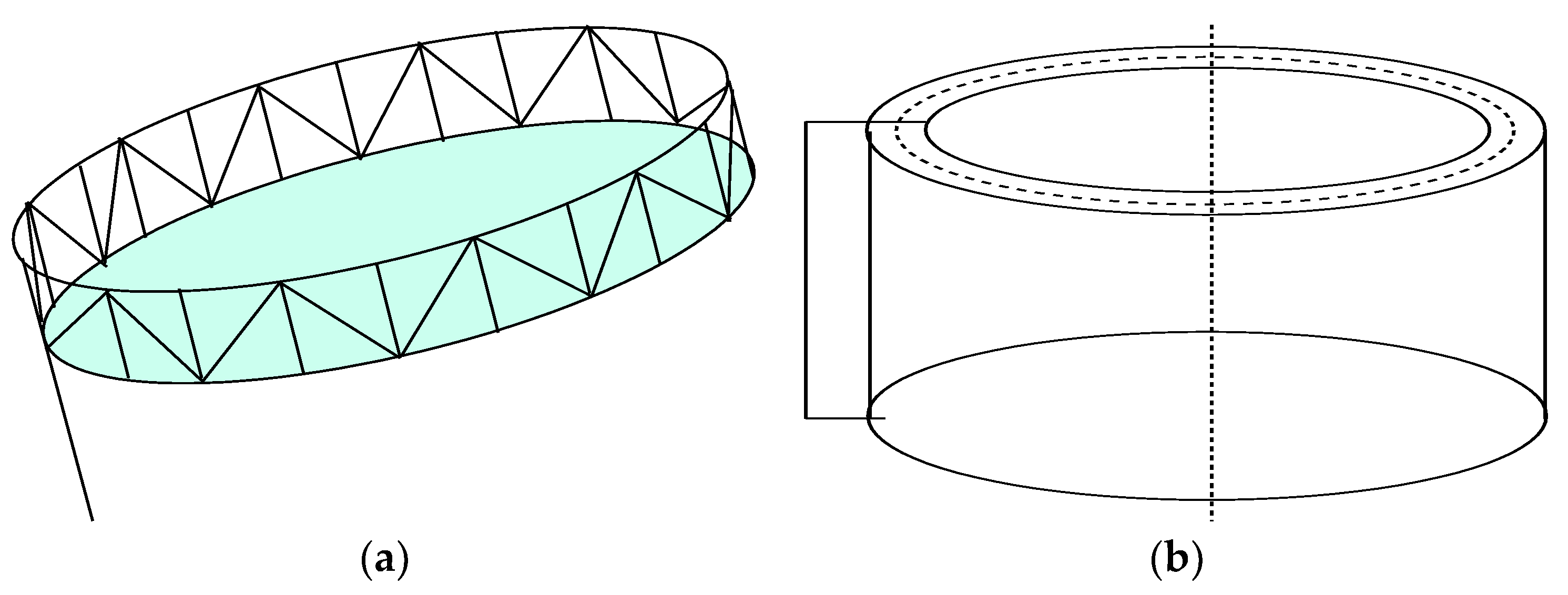
To demonstrate the applicability and effectiveness of our theoretical results, the periodic breath vibrations of a two-degree-of-freedom mechanical model of the circular mesh antenna subjected to the thermal excitation are investigated. An equivalent circular cylindrical shell model is regarded as a simplified model of the circular mesh antenna, as shown in Figure 1 [30].
Based on Reddy’s first-order shear deformation theorem, Hamilton’s principle, and the Galerkin procedure, a two-degree-of-freedom dynamic system of the circular cylindrical shell is obtained as follows [30]:
where and are frictional coefficients, is thermal excitation, and and are two linear frequencies.
Considering the case of primary parameter resonance and 1:1 internal resonance, we have the relations
where , are detuning parameters. Supposing for convenience, introducing the scale transformations
and denoting the asymptotic solutions of System (26) as
we obtain
where , . Writing
the averaged equations are obtained based on normal form theory and the method of multiple scales:
By introducing the transformations
if , System (27) can be rewritten as
Now System (28) is in the form of System (1) and the degree of its homogeneous terms is three, which shows that . Supposing , we discuss the periodic solutions of System (28) by considering the cases of , , and , where: .
(1)
. Based on Lemma 5, we obtain:
The following two statements hold for System (28): (1) If , then and the periodic solutions cannot be obtained by Theorem 3; (2) If , then and the number of periodic solutions is 1 and 0 if and , respectively.
(2)
. Now is odd, and System (28) has no periodic solution based on Theorem 2.
(3)
. Based on Lemma 5, we obtain . Hence, System (28) has no periodic solution in this case based on Theorem 3.
To verify the effectiveness of our results, we detect the phase portraits of the periodic solutions of System (28) under a group of parameter conditions via numerical simulations. Considering the parameter condition
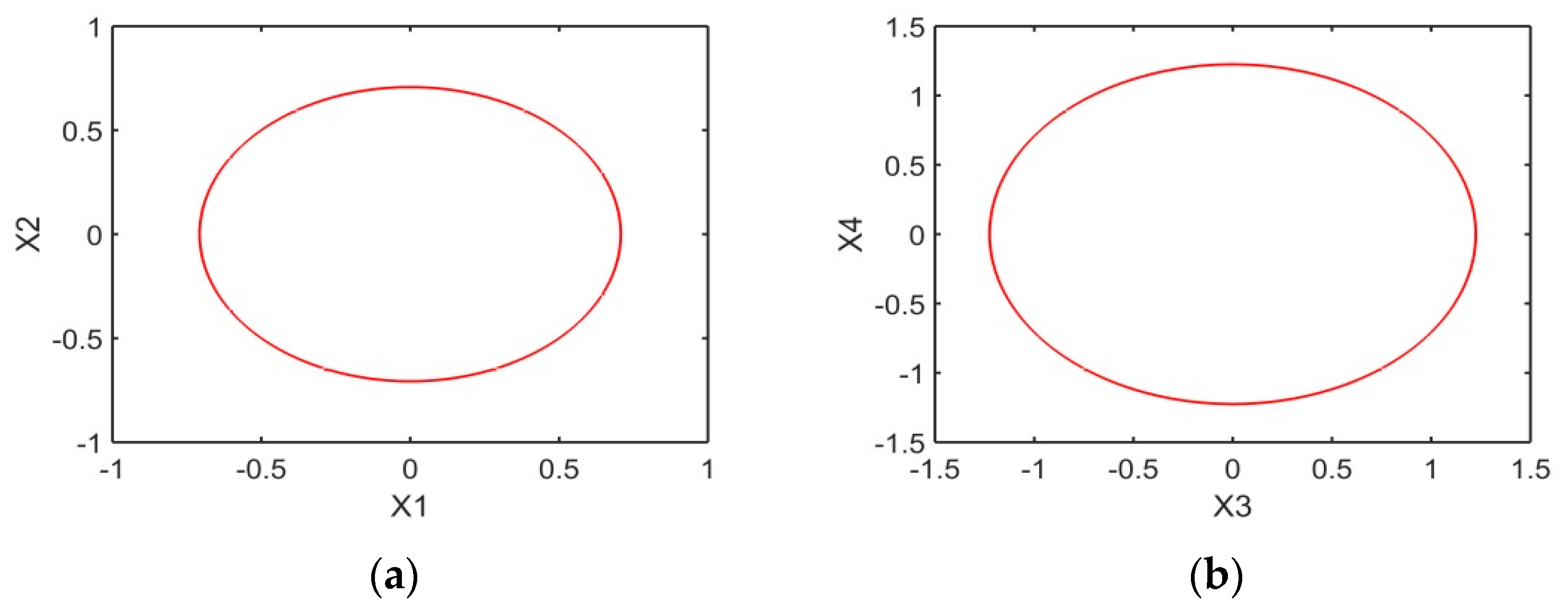
when , System (28) has one periodic solution for and no periodic solution for ; when and , System (28) has no periodic solution. Next, we show the phase portraits of the one periodic solution of System (28) in the case of and . Figure 2a,b respectively demonstrate the projections of the periodic solution on the plans and , and Figure 2c,d show the phase portraits in space and for .
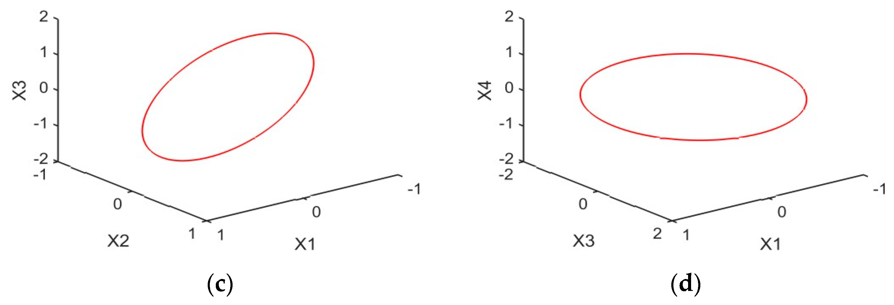
Figure 3 shows the phase portraits of the periodic solution of System (28) for and .
The exact number and parameter control conditions of the periodic solutions of System (28) are obtained based on theoretical and numerical methods, which can provide a detailed description for the periodic solutions when the coefficients are allowed to vary in a wide range of parameters. Based on numerical simulations, under the parameter condition (), the phase portraits of the periodic solutions with different values of can be observed from Figure 2 and Figure 3, which can verify the theoretical and numerical results. The obtained results show new understanding on the periodic motions of the circular mesh antenna and provide a method for vibration control.
5. Conclusions
In this paper, the periodic solutions for a four-dimensional coupled polynomial system with N-degree homogeneous nonlinearities are investigated. When the unperturbed linear part of the four-dimensional system has a center singular point in generalization resonance at the origin for , , , the new explicit expression of the displacement function of order is obtained by introducing the exact formulas on power trigonometric integrals, which is in agreement with certain existing results, but we obtain the more detailed expression by including the exact coefficients. By considering the zero solutions of with complex coefficient relations, the results on the existence condition, exact number, and parameter control conditions of the periodic solutions of System (1) are obtained, which shows that the parity of has a great influence on the periodic solutions. Results obtained in this paper provide more precise and detailed bifurcation information for System (1) than the existing results in the case of , which can be widely applied to various engineering applications and help engineers better analyze the complex periodic vibrations exhibited in reality. Theorems 1–3 verify and improve the upper bound of the number of periodic solutions obtained in the previous literature for System (1), which presents the effects of important parameters on the phenomena of the emergence and disappearance of periodic solutions and shows a new theoretical explanation on vibration mechanisms.
As an application, the periodic solutions of a two-degree-of-freedom circular mesh antenna model subjected to the thermal excitation are investigated by theoretical and numerical methods. The results on the exact number, parameter control conditions, and the relative positions of the periodic solutions are obtained, which verify the applicability and validity of the theoretical results and show the complicated periodic motions of circular mesh antenna. Periodic vibrations with high amplitudes may lead to serious damage to the device, and the theoretical results obtained in this paper may provide a parameter method for vibration control of circular mesh antenna.
It is remarkable that the method for detecting the existence of periodic solutions of System (1) can also be extended to the four-dimensional system with m-degree nonhomogeneous terms:
where , , and the other expressions , , and have the same meaning as those exhibited in System (1). Lemma 5 provides a convenient way to compute the expression , where
Hence, we can obtain a result similar to Theorem 1. However, due to the complex coefficients of , research on the exact number and parameter control conditions of periodic solutions of System (29) is still a difficult topic that will be investigated in a further study. In addition, some higher dimensional (odd or even) systems have arisen more and more frequently in the fields of science and engineering in recent years, so we will try to study their periodic solutions as well as the stability in later work.
Author Contributions
All authors are contributing equally to this research.
Funding
The research project is supported by the National Natural Science Foundation of China (11772007, 11372014, 11571026 and 11290152) and is also supported by the Beijing Natural Science Foundation (1172002, Z180005 and 1192003).
Conflicts of Interest
The authors declare no conflict of interest.
References
Avramov, K.V.; Mikhlin, Y.V.; Kurilov, E. Asymptotic analysis of nonlinear dynamics of simply supported cylindrical shells. Nonlinear Dyn.2007, 47, 331–352. [Google Scholar] [CrossRef]
Li, J.B. Hilbert’s 16th problem and bifurcations of planar polynomial vector fields. Int. J. Bifurc. Chaos2003, 13, 47–106. [Google Scholar] [CrossRef]
An, Y.L.; Han, M.A. On the number of limit cycles near a homoclinic loop with a nilpotent singular point. J. Differ. Equ.2015, 258, 3194–3247. [Google Scholar] [CrossRef]
Yang, J.M.; Ding, W. Limit cycles of a class of Lienard systems with restoring forces of seventh degree. Appl. Math. Comput.2018, 316, 422–437. [Google Scholar] [CrossRef]
Da Cruz, L.P.C.; Novaes, D.D.; Torregrosa, J. New lower bound for the Hilbert number in piecewise quadratic differential systems. J. Differ. Equ.2019, 266, 4170–4203. [Google Scholar] [CrossRef]
Bey, M.; Badi, S.; Fernane, K.; Makhlouf, A. The number of limit cycles bifurcating from the periodic orbits of an isochronous center. Math. Methods Appl. Sci.2019, 42, 821–829. [Google Scholar] [CrossRef]
Kadry, S.; Alferov, G.; Ivanov, G.; Korolev, V.; Selitskaya, V. A new method to study the periodic solutions of the ordinary differential equations using functional analysis. Mathematics2019, 7, 677. [Google Scholar] [CrossRef]
Poincaré, H. Les Méthodes Nouvelles de la Mécanique Celeste; Gauthier: Paris, France, 1899. [Google Scholar]
Veerman, P.; Holmes, P. The existence of arbitrarily many distinct periodic orbits in a two degree of freedom Hamiltonian system. Physica D1985, 14, 177–192. [Google Scholar] [CrossRef]
Nayfeh, A.H.; Balachandran, A.B. Applied Nonlinear Dynamics; Wiley: New York, NY, USA, 1995. [Google Scholar]
Sanders, J.A.; Verhulst, F.; Murdock, J. Averaging Methods in Nonlinear Dynamical Systems; Springer: New York, NY, USA, 2007. [Google Scholar]
Mahdi, A.; Romanovski, V.G.; Shafer, D.S. Stability and periodic oscillations in the Moon-Rand systems. Nonlinear Anal. Real World Appl.2013, 14, 294–313. [Google Scholar] [CrossRef][Green Version]
Wang, L.X.; Zhang, J.M.; Shao, H.J. Existence and global stability of a periodic solution for a cellular neural network. Nonlinear Sci. Numer. Simul.2014, 19, 2983–2992. [Google Scholar] [CrossRef]
Zhang, J.M.; Zhang, L.J.; Bai, Y.Z. Stability and bifurcation analysis on a predator–prey system with the weak Allee effect. Mathematics2019, 7, 432. [Google Scholar] [CrossRef]
Wiggins, S.; Holmes, P. Homoclinic orbits in slowly varying oscillators. SIAM J. Appl. Math.1987, 18, 592–611. [Google Scholar] [CrossRef]
Ye, Z.Y.; Han, M.A. Bifurcations of invariant tori and subharmonic solutions of singularly perturbed system. Chin. Ann. Math. Ser. B2007, 28, 135–148. [Google Scholar] [CrossRef]
Chiba, H. Periodic orbits and chaos in fast-slow systems with Bogdanov-Takens type fold points. J. Differ. Equ.2011, 250, 112–160. [Google Scholar] [CrossRef]
Sourdis, C. On periodic orbits in a slow-fast system with normally elliptic slow manifold. Math. Mehtods Appl. Sci.2014, 37, 270–276. [Google Scholar] [CrossRef]
Tian, H.H.; Han, M.A. Bifurcation of periodic orbits by perturbing high-dimensional piecewise smooth integrable systems. J. Differ. Equ.2017, 263, 7448–7474. [Google Scholar] [CrossRef]
Sun, M.; Zhang, W.; Chen, J.E.; Yao, M.H. Subharmonic Melnikov theory for degenerate resonance systems and its application. Nonlinear Dyn.2017, 89, 1173–1186. [Google Scholar] [CrossRef]
Wang, Q.L.; Huang, W.T.; Liu, Y.R. Multiple limit cycles bifurcation from the degenerate singularity for a class of three-dimensional systems. Acta Math. Appl. Sin. Engl. Ser.2016, 32, 73–80. [Google Scholar] [CrossRef]
Li, J.; Quan, T.T.; Zhang, W. Bifurcation and number of subharmonic solutions of a 4D non-autonomous slow–fast system and its application. Nonlinear Dyn.2018, 92, 721–739. [Google Scholar] [CrossRef]
Cheng, Y.Y. Bifurcation of limit cycles of a class of piecewise linear differential systems in R4 with three zones. Discrete Dyn. Nat. Soc.2013, 2013. [Google Scholar] [CrossRef]
Navarro, J.F.; Poveda, R. Computation of periodic orbits in three-dimensional Lotka-Volterra systems. Math. Methods Appl. Sci.2017, 40, 7185–7200. [Google Scholar] [CrossRef]
Barreira, L.; Llibre, J.; Valls, C. Bifurcation of limit cycles from a 4-dimensional center in Rm in resonance 1: N. J. Math. Anal. Appl.2012, 389, 754–768. [Google Scholar] [CrossRef]
Chen, Y.M.; Liang, H.H. Zero-zero-Hopf bifurcation and ultimate bound estimation of a generalized Lorenz–Stenflo hyperchaotic system. Math. Methods. Appl. Sci.2017, 40, 3424–3432. [Google Scholar] [CrossRef]
Barreira, L.; Llibre, J.; Valls, C. Limit cycles bifurcating from a zero–Hopf singularity in arbitrary dimension. Nonlinear Dyn.2018, 92, 1159–1166. [Google Scholar] [CrossRef]
Zhang, W.; Chen, J.; Wang, Y.F.; Yang, X.D. Continuous model and nonlinear dynamic responses of circular mesh antenna clamped at one side. Eng. Struct.2017, 151, 115–135. [Google Scholar] [CrossRef]
Figure 1.
(a) The circular mesh antenna; (b) The equivalent circular cylindrical shell.
Figure 1.
(a) The circular mesh antenna; (b) The equivalent circular cylindrical shell.
Figure 2.
Periodic solution of System (28) with : (a) on the plane ; (b) on the plane ; (c) in space ; (d) in space .
Figure 2.
Periodic solution of System (28) with : (a) on the plane ; (b) on the plane ; (c) in space ; (d) in space .
Figure 3.
Periodic solution of System (28) with : (a) on the plane ; (b) on the plane ; (c) in space ; (d) in space .
Figure 3.
Periodic solution of System (28) with : (a) on the plane ; (b) on the plane ; (c) in space ; (d) in space .
Tian, Y.; Li, J.
Periodic Solutions for a Four-Dimensional Coupled Polynomial System with N-Degree Homogeneous Nonlinearities. Mathematics2019, 7, 1218.
https://doi.org/10.3390/math7121218
AMA Style
Tian Y, Li J.
Periodic Solutions for a Four-Dimensional Coupled Polynomial System with N-Degree Homogeneous Nonlinearities. Mathematics. 2019; 7(12):1218.
https://doi.org/10.3390/math7121218
Chicago/Turabian Style
Tian, Yuanyuan, and Jing Li.
2019. "Periodic Solutions for a Four-Dimensional Coupled Polynomial System with N-Degree Homogeneous Nonlinearities" Mathematics 7, no. 12: 1218.
https://doi.org/10.3390/math7121218
APA Style
Tian, Y., & Li, J.
(2019). Periodic Solutions for a Four-Dimensional Coupled Polynomial System with N-Degree Homogeneous Nonlinearities. Mathematics, 7(12), 1218.
https://doi.org/10.3390/math7121218
Note that from the first issue of 2016, this journal uses article numbers instead of page numbers. See further details here.
Article Metrics
No
No
Article Access Statistics
For more information on the journal statistics, click here.
Multiple requests from the same IP address are counted as one view.
Tian, Y.; Li, J.
Periodic Solutions for a Four-Dimensional Coupled Polynomial System with N-Degree Homogeneous Nonlinearities. Mathematics2019, 7, 1218.
https://doi.org/10.3390/math7121218
AMA Style
Tian Y, Li J.
Periodic Solutions for a Four-Dimensional Coupled Polynomial System with N-Degree Homogeneous Nonlinearities. Mathematics. 2019; 7(12):1218.
https://doi.org/10.3390/math7121218
Chicago/Turabian Style
Tian, Yuanyuan, and Jing Li.
2019. "Periodic Solutions for a Four-Dimensional Coupled Polynomial System with N-Degree Homogeneous Nonlinearities" Mathematics 7, no. 12: 1218.
https://doi.org/10.3390/math7121218
APA Style
Tian, Y., & Li, J.
(2019). Periodic Solutions for a Four-Dimensional Coupled Polynomial System with N-Degree Homogeneous Nonlinearities. Mathematics, 7(12), 1218.
https://doi.org/10.3390/math7121218
Note that from the first issue of 2016, this journal uses article numbers instead of page numbers. See further details here.


