Simplified Fractional Order Controller Design Algorithm


Abstract
1. Introduction
- Phase margin φm and gain crossover frequency ωcg:
- Iso-damping property;
- High-frequency noise rejection;
- Good output disturbance rejection; and
- Steady-state error cancellation;
- ; ;
- ;
- , with A the desired noise attenuation for frequencies rad/s;
- , with B the desired value of the sensitivity function for frequencies rad/s.
2. The Proposed Controller Design Method
2.1. The Generalized Optimum Method
2.2. Fractional Order Optimum Method
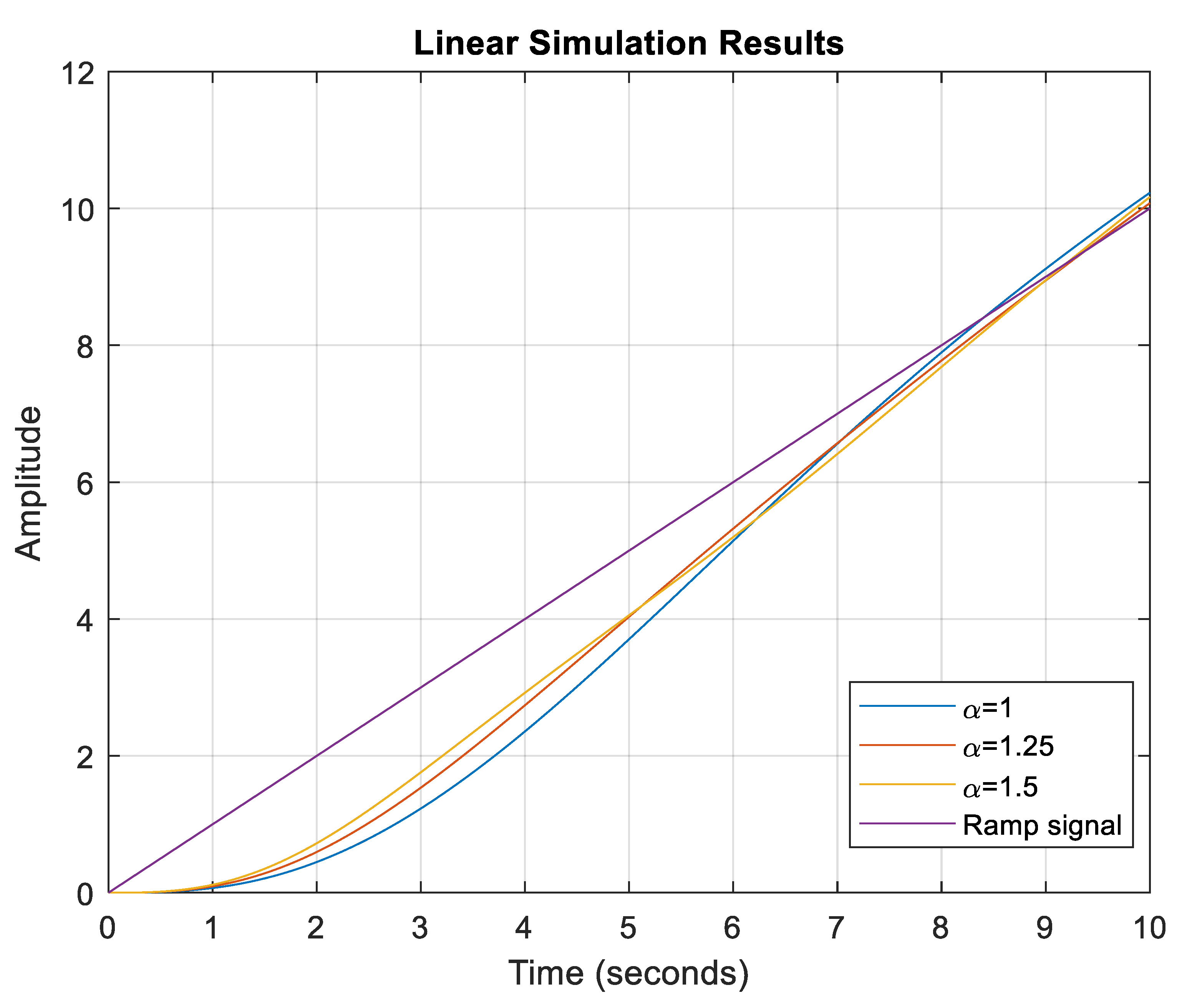
- Having the process mathematical model of the form of Equation (5), the open loop transfer function form is imposed as in Equation (16) to provide zero steady-state position and velocity error.
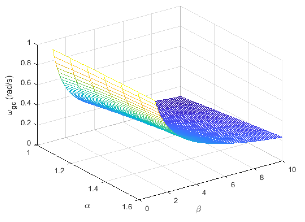
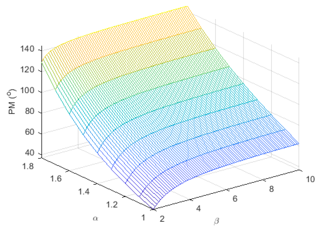
- Using Equations (18) and (19) the tuning parameters K, α and β for the desired values of gain crossover frequency and phase margin are computed.
- Having the open loop in Equation (17) and the process model in Equation (5), the transfer function of the fractional order controller in one of the forms presented in [22] is obtained.
3. Case Studies
3.1. Integer Order Plant, without Zero
3.2. Integer Order Plant with Zero
3.3. Fractional Order Plant
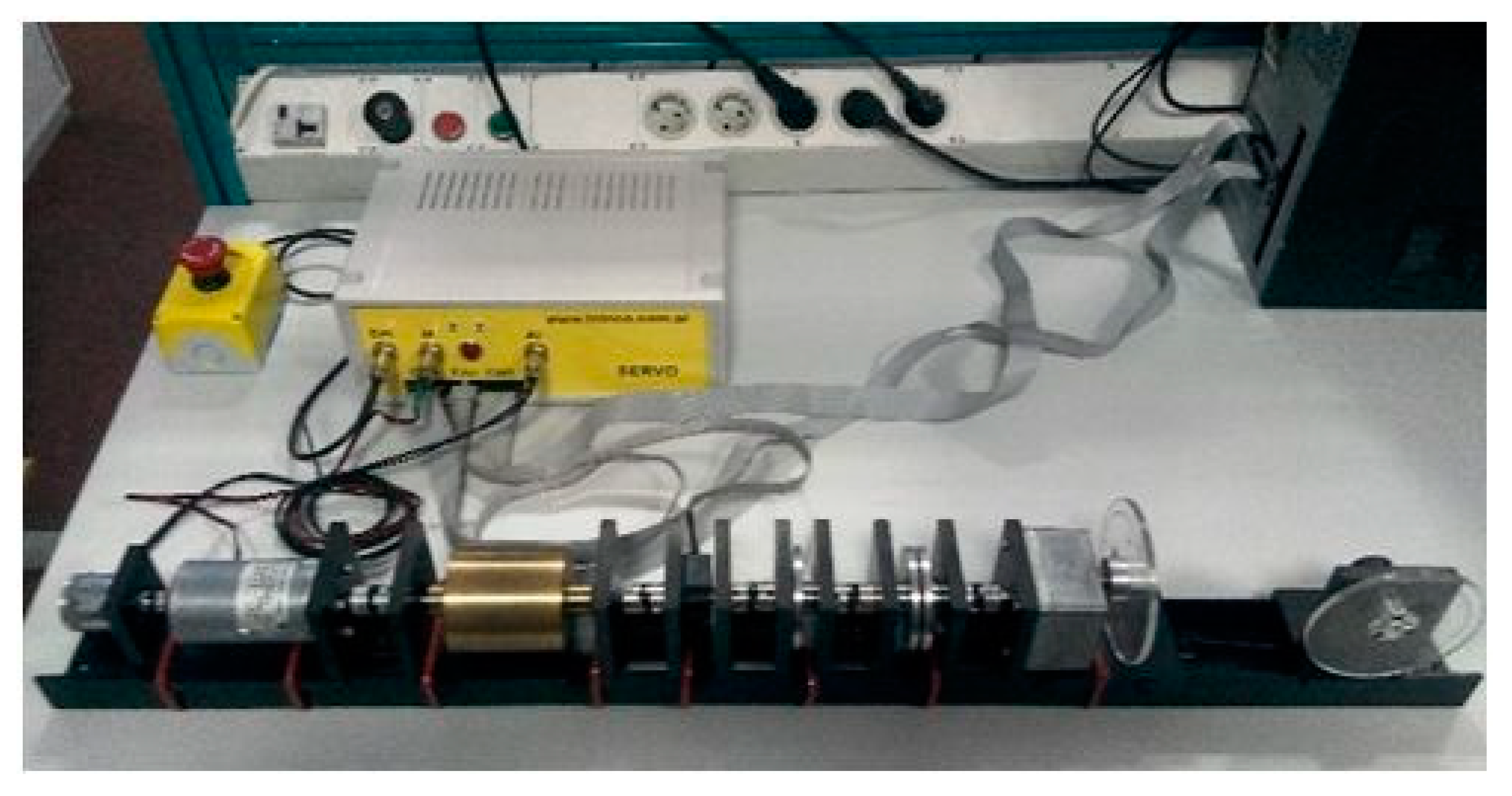
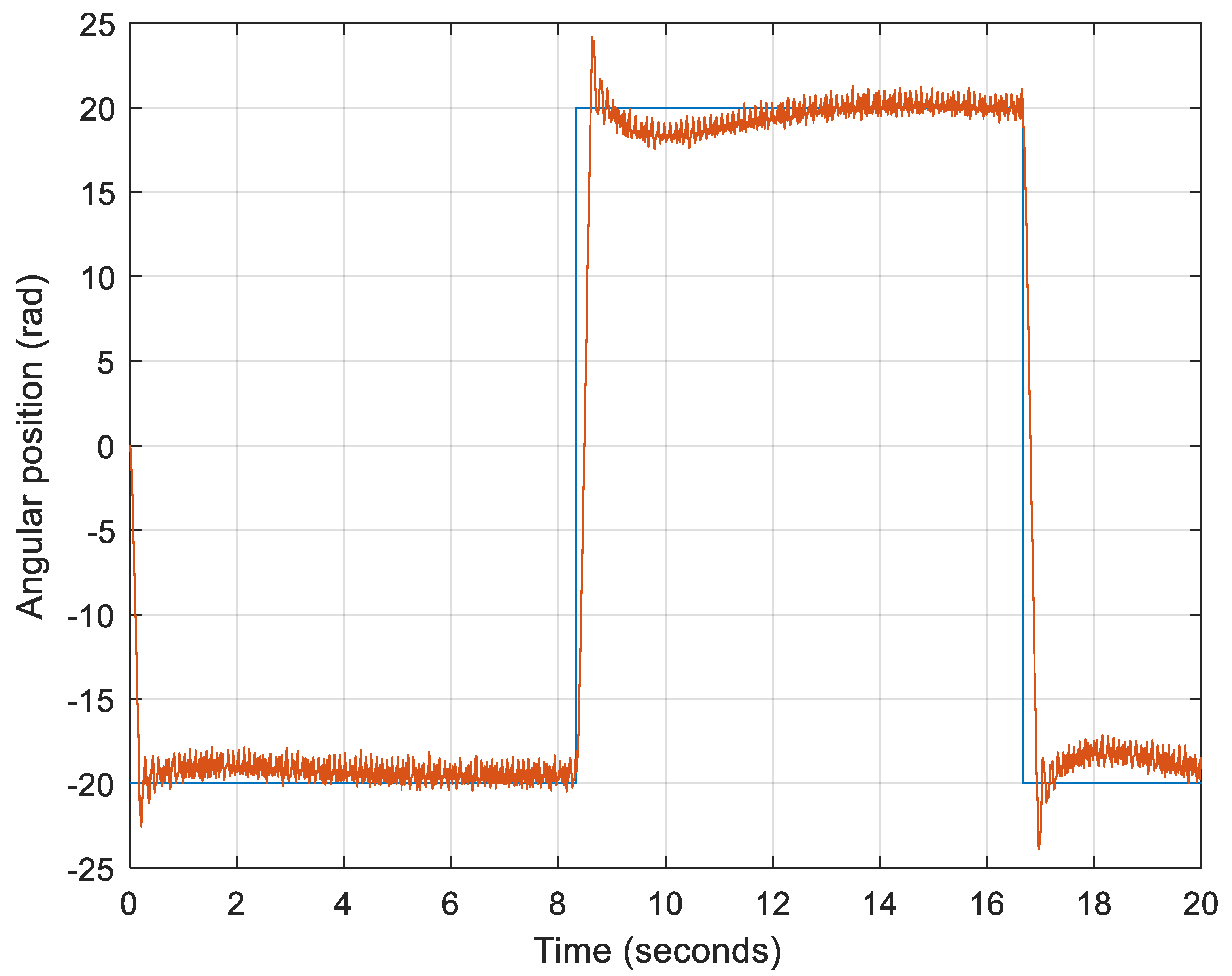
3.4. Experimental Case Study
4. Conclusions
- Ensures practically any closed loop performance measures, given the possibility to choose the most convenient solution by optimization for the tuning parameters α and β. Each solution will ensure the maximum possible value of the phase margin.
- It is a simple method of the same complexity as the Kessler’s optimum method.
- It can be applied for practically any type of process model, from integer order models to fractional order models, which can be approximated as in Equation (9).
Funding
Acknowledgments
Conflicts of Interest
References
- Chen, Y.Q.; Petras, I.; Xue, D. Fractional order control-A tutorial. In Proceedings of the 2009 American Control Conference, St. Louis, MO, USA, 10–12 June 2009; pp. 1397–1411. [Google Scholar]
- Tejado, I.; Vinagre, B.M.; Traver, J.E.; Prieto-Arranz, J.; Nuevo-Gallardo, C. Back to Basics: Meaning of the Parameters of Fractional Order PID Controllers. Mathematics 2019, 7, 530. [Google Scholar] [CrossRef]
- Petráš, I.; Terpák, J. Fractional Calculus as a Simple Tool for Modeling and Analysis of Long Memory Process in Industry. Mathematics 2019, 7, 511. [Google Scholar] [CrossRef]
- Gutiérrez, R.E.; Rosário, J.M.; Machado, J.T. Fractional Order Calculus: Basic Concepts and Engineering Applications. Math. Probl. Eng. 2010, 2010, 375858. [Google Scholar] [CrossRef]
- Fathalla, A.R. Numerical Modeling of Fractional-Order Biological Systems. Abstr. Appl. Anal. 2013, 2013, 816803. [Google Scholar] [CrossRef]
- Hilfer, R. Applications of Fractional Calculus in Physics; World Scientific: Singapore, Singapore, 2000. [Google Scholar] [CrossRef]
- Miller, K.S.; Ross, B. An Introduction to the Fractional Calculus and Fractional Differential Equations; John Wiley & Sons: New York, NY, USA, 1993. [Google Scholar]
- Podlubny, I. Fractional-order systems and PIλDμ-controllers. IEEE Trans. Autom. Control. 1999, 44, 208–213. [Google Scholar] [CrossRef]
- Oustaloup, A. La Commande CRONE; Editions HERMES: Paris, France, 1991. [Google Scholar]
- Bruzzone, L.; Fanghella, P. Fractional-Order Control of a Micrometric Linear Axis. J. Control. Sci. Eng. 2013, 2013, 947428. [Google Scholar] [CrossRef]
- Bruzzone, L.; Fanghella, P. Comparison of PDD1/2 and PDu Position Controls of a Second Order Linear System. In Proceedings of the 33rd IASTED International Conference on Modelling, Identification and Control MIC 2014, Innsbruck, Austria, 17–19 February 2014; pp. 182–188. [Google Scholar]
- Monje, C.A.; Chen, Y.Q.; Vinagre, B.M.; Xue, D.; Feliu-Batlle, V. Fundamentals of Fractional-Order Systems; Springer: London, UK, 2010. [Google Scholar]
- Dulf, E.H.; Timis, D.; Muresan, C.I. Robust Fractional Order Controllers for Distributed Systems. Acta Polytech. Hung. 2017, 14, 163–176. [Google Scholar]
- Muresan, C.I.; Dulf, E.H.; Both, R. Vector-based tuning and experimental validation of fractional-order PI/PD controllers. Nonlinear Dyn. 2016, 84, 179–188. [Google Scholar] [CrossRef]
- Padula, F.; Visioli, A. Tuning rules for optimal PID and fractional-order PID controllers. J. Process Control 2011, 21, 69–81. [Google Scholar] [CrossRef]
- Valerio, D.; da Costa, J.S. Tuning of fractional PID controllers with Ziegler Nichols-type rules. Signal Process. 2006, 86, 2771–2784. [Google Scholar] [CrossRef]
- Hmed, A.B.; Amairi, M.; Aoun, M.; Hamdi, S.E. Comparative study of some fractional PI controllers for first order plus time delay systems. In Proceedings of the 2017 18th International Conference on Sciences and Techniques of Automatic Control and Computer Engineering (STA), Monastir, Tunisia, 21–23 December 2017; pp. 278–283. [Google Scholar]
- Garrappa, R.; Kaslik, E.; Popolizio, M. Evaluation of Fractional Integrals and Derivatives of Elementary Functions: Overview and Tutorial. Mathematics 2019, 7, 407. [Google Scholar] [CrossRef]
- Kessler, C. Das symmetrische Optimum. Regelungstechnik 1958, 6, 432–436. [Google Scholar]
- Voda, A.A.; Landau, I.D. A Method for the Auto-calibration of PID Controllers. Automatica 1995, 31, 41–53. [Google Scholar] [CrossRef]
- Preitl, S.; Precup, R.E. An extension of tuning relations after symmetrical optimum method for PI and PID controllers. Automatica 1999, 35, 1731–1736. [Google Scholar] [CrossRef]
- Ahmadi Dastjerdi, A.; Vinagre, B.M.; Chen, Y.Q.; HosseinNia, S.H. Linear fractional order controllers; A survey in the frequency domain. Annu. Rev. Control 2019, 47, 51–70. [Google Scholar] [CrossRef]
- Oustaloup, A.; Levron, F.; Mathieu, B.; Nanot, F.M. Frequency-band complex noninteger differentiator: Characterization and synthesis. IEEE Trans. Circuits Syst. I 2000, 47, 25–39. [Google Scholar] [CrossRef]
- Oustaloup, A.; Sabatier, J.; Lanusse, P.; Malti, R.; Melchior, P.; Moreau, X.; Moze, M. An overview of the crone approach in system analysis, modeling and identification, observation and control. IFAC Proc. 2008, 41, 14254–14265. [Google Scholar] [CrossRef]
- Inteco, Poland. Modular Servo System-User’s Manual. Available online: www.inteco.com.pl (accessed on 26 August 2019).


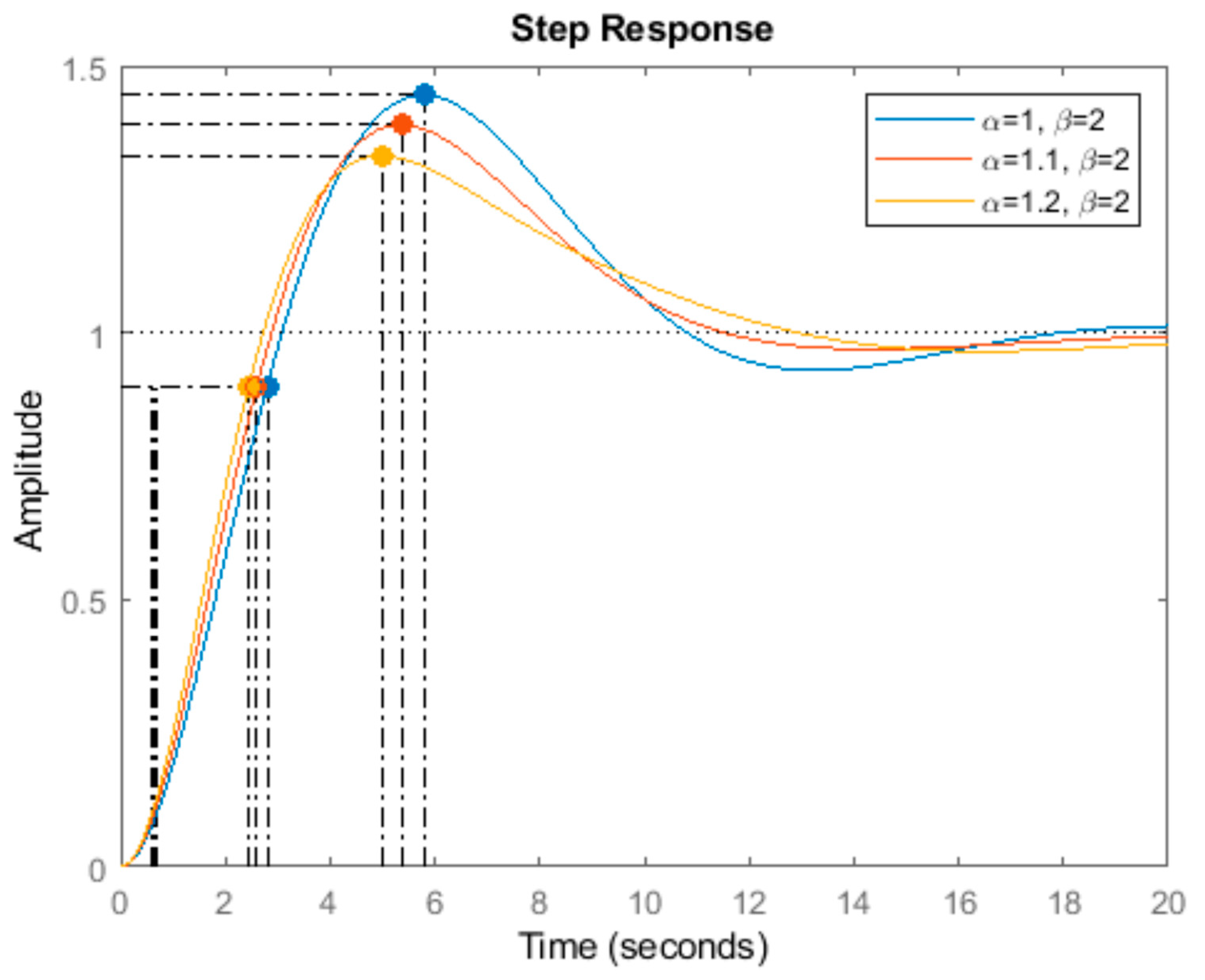
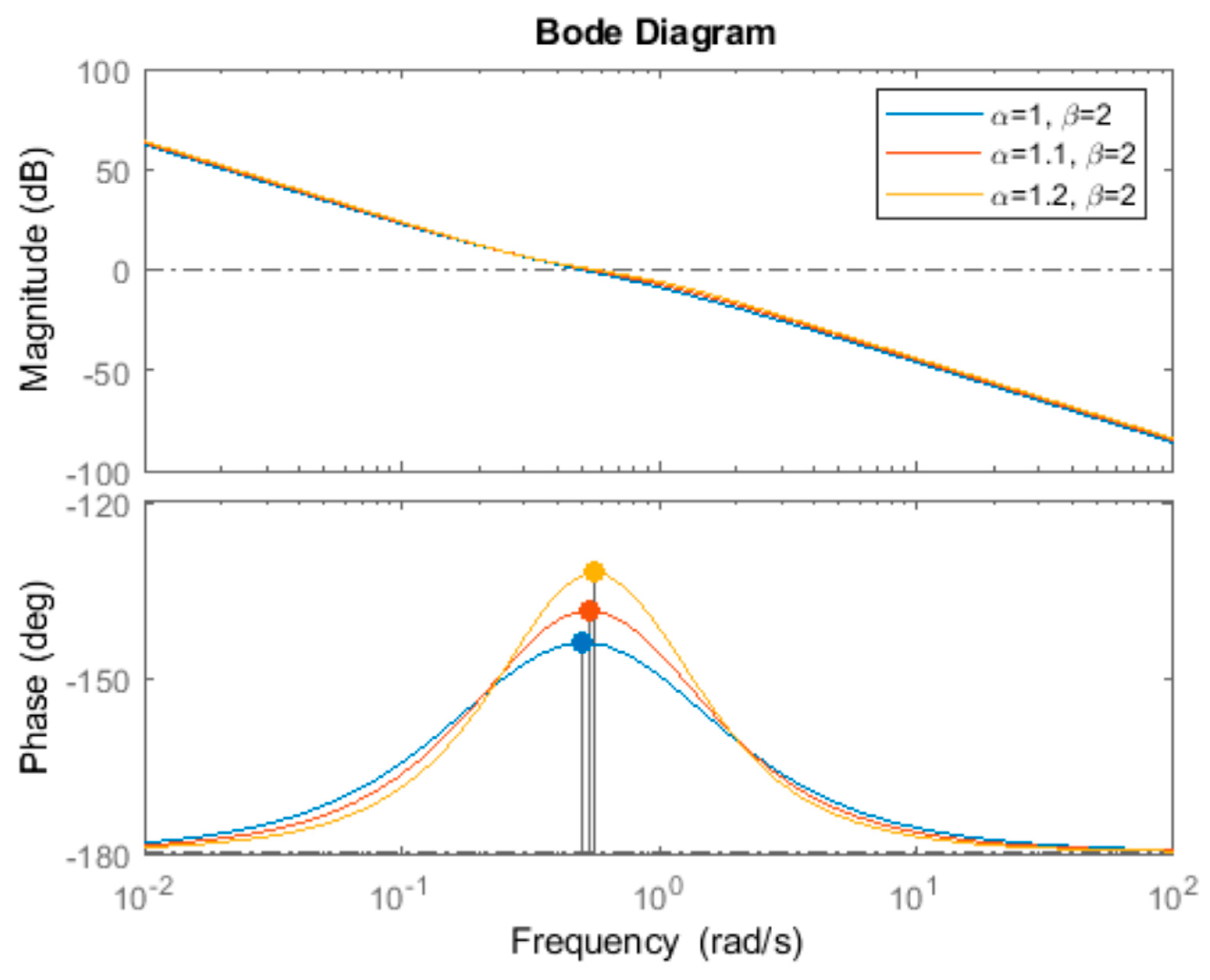
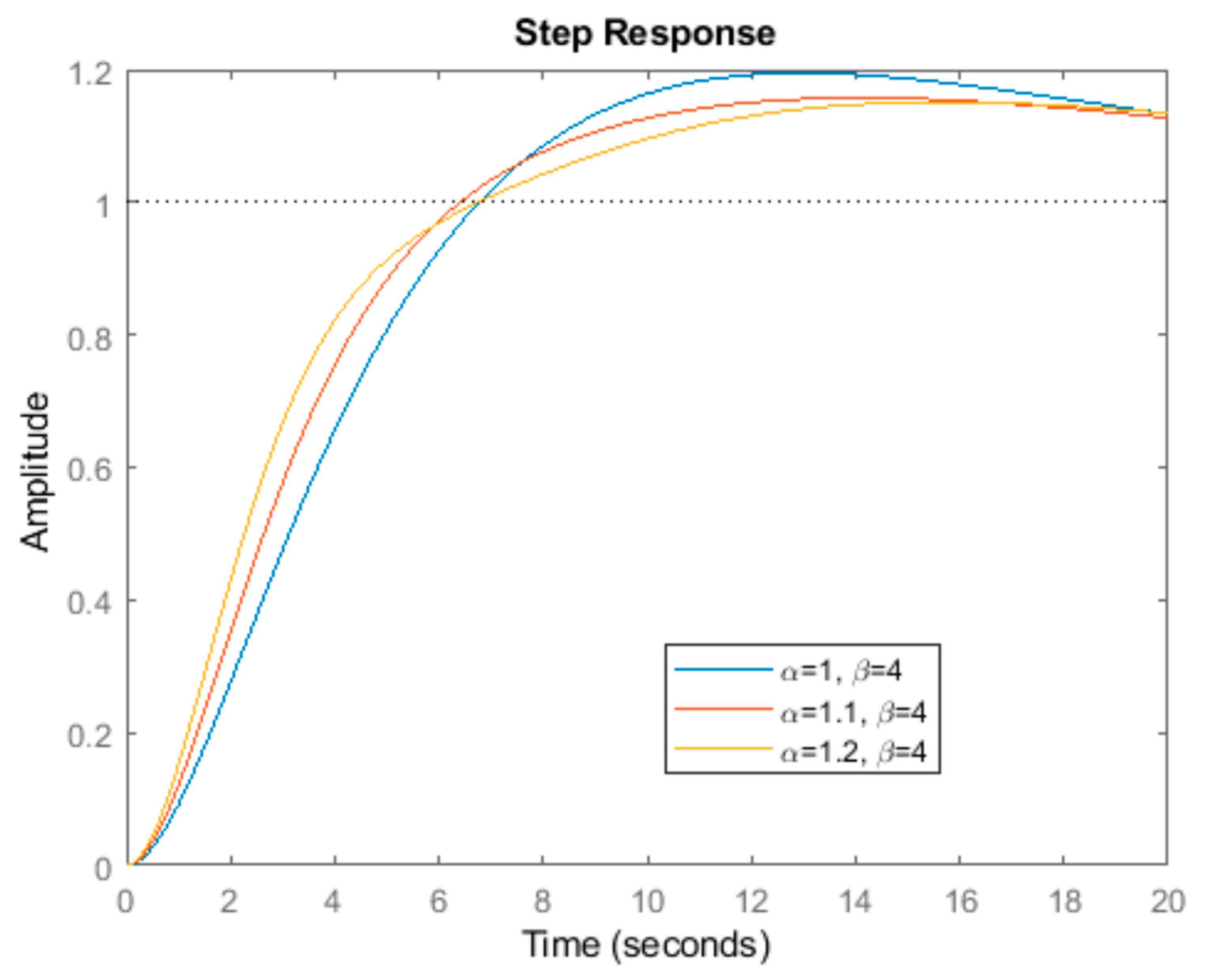
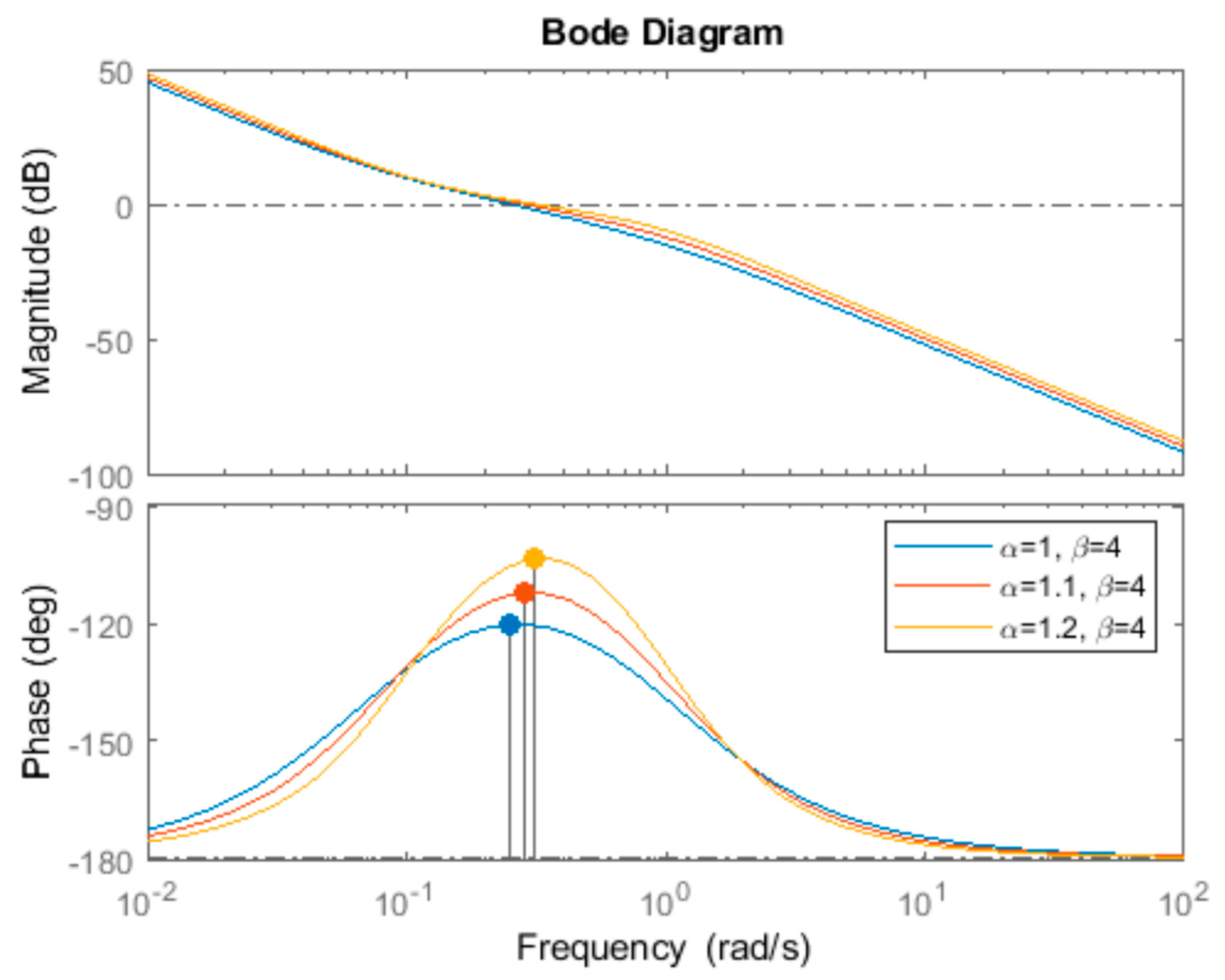
| α | Gain Crossover Frequency (rad/s) | Phase Margin (°) | Overshoot (%) | Rise Time (s) | |
|---|---|---|---|---|---|
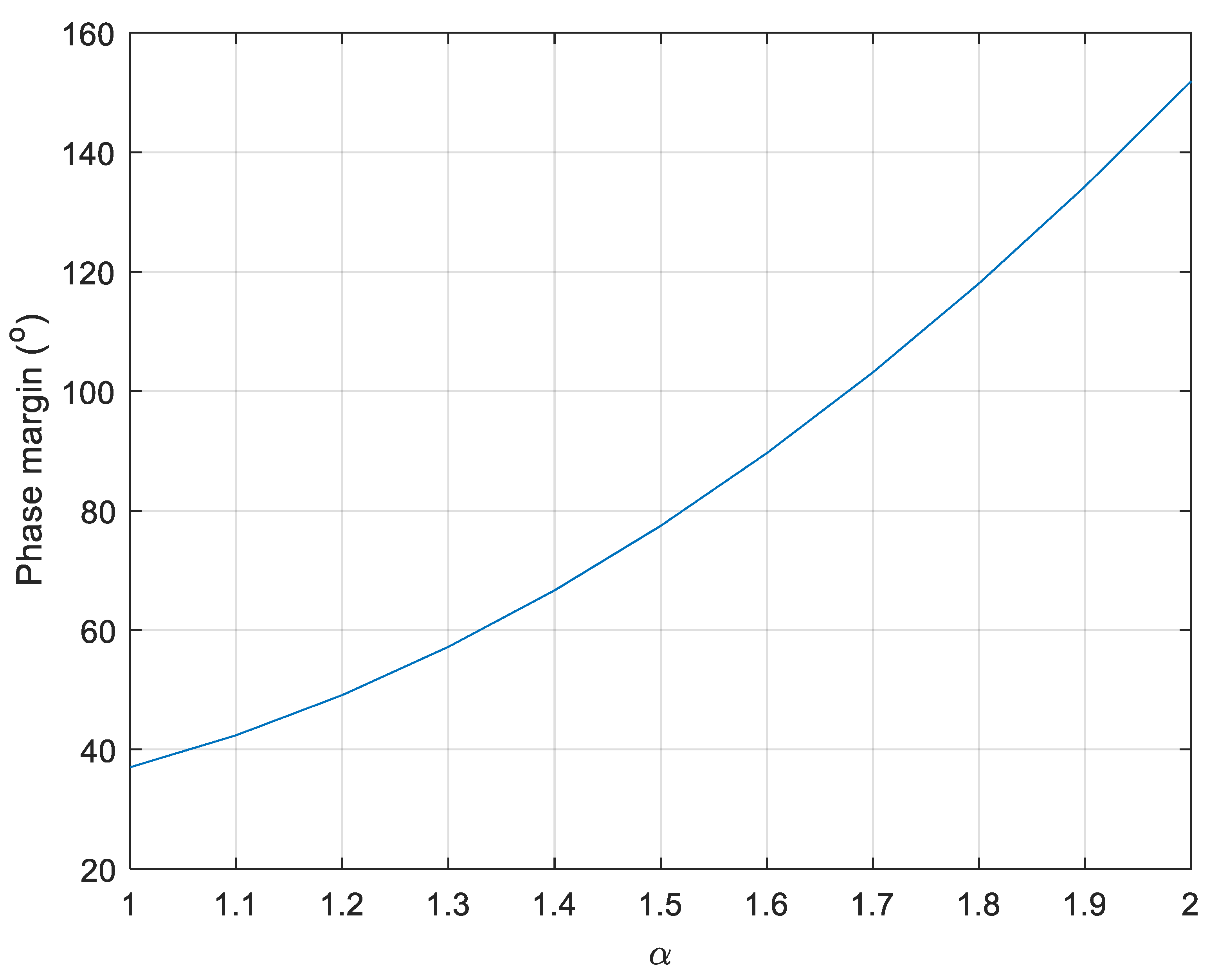
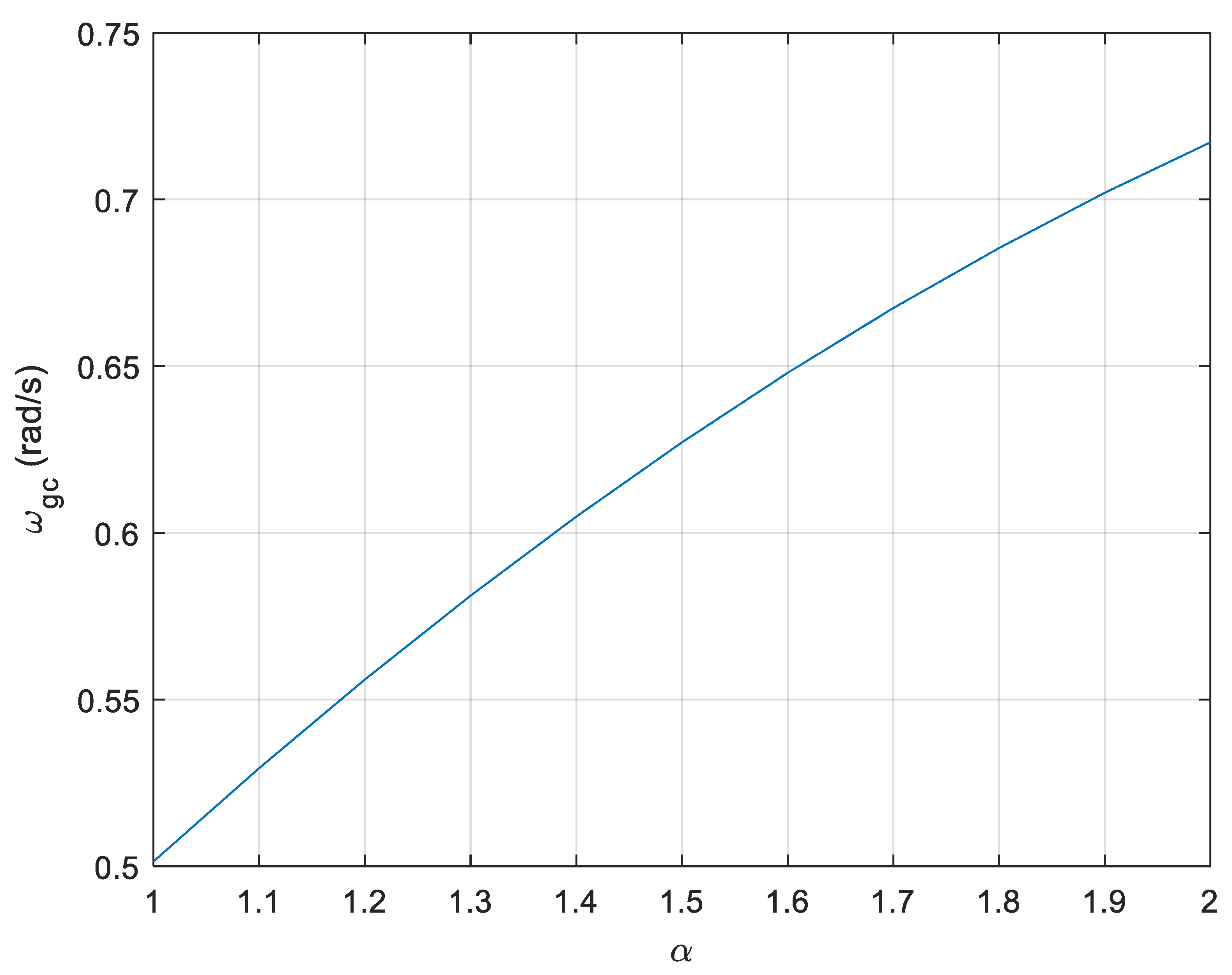
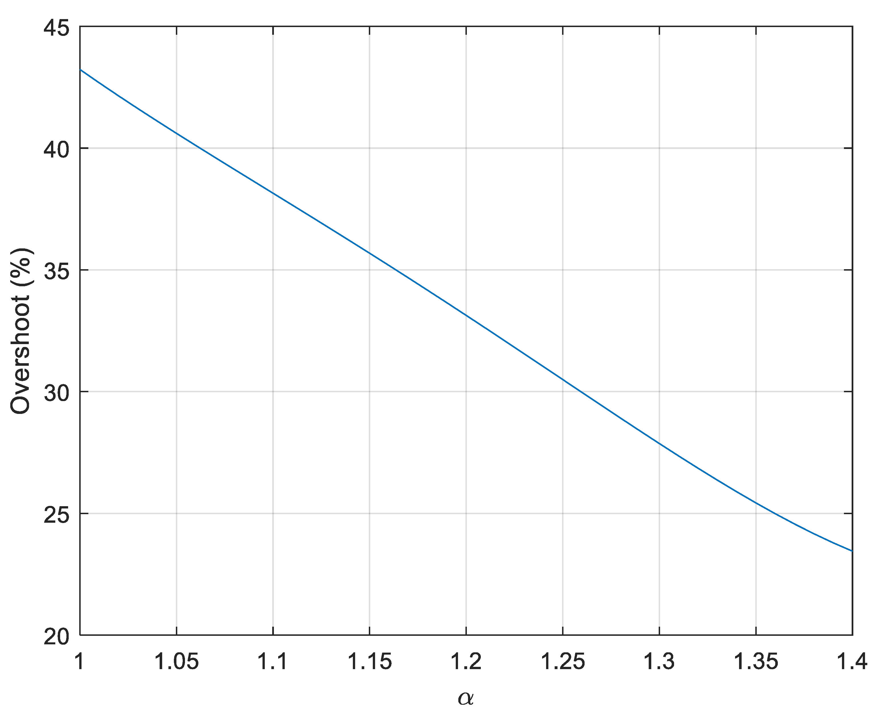
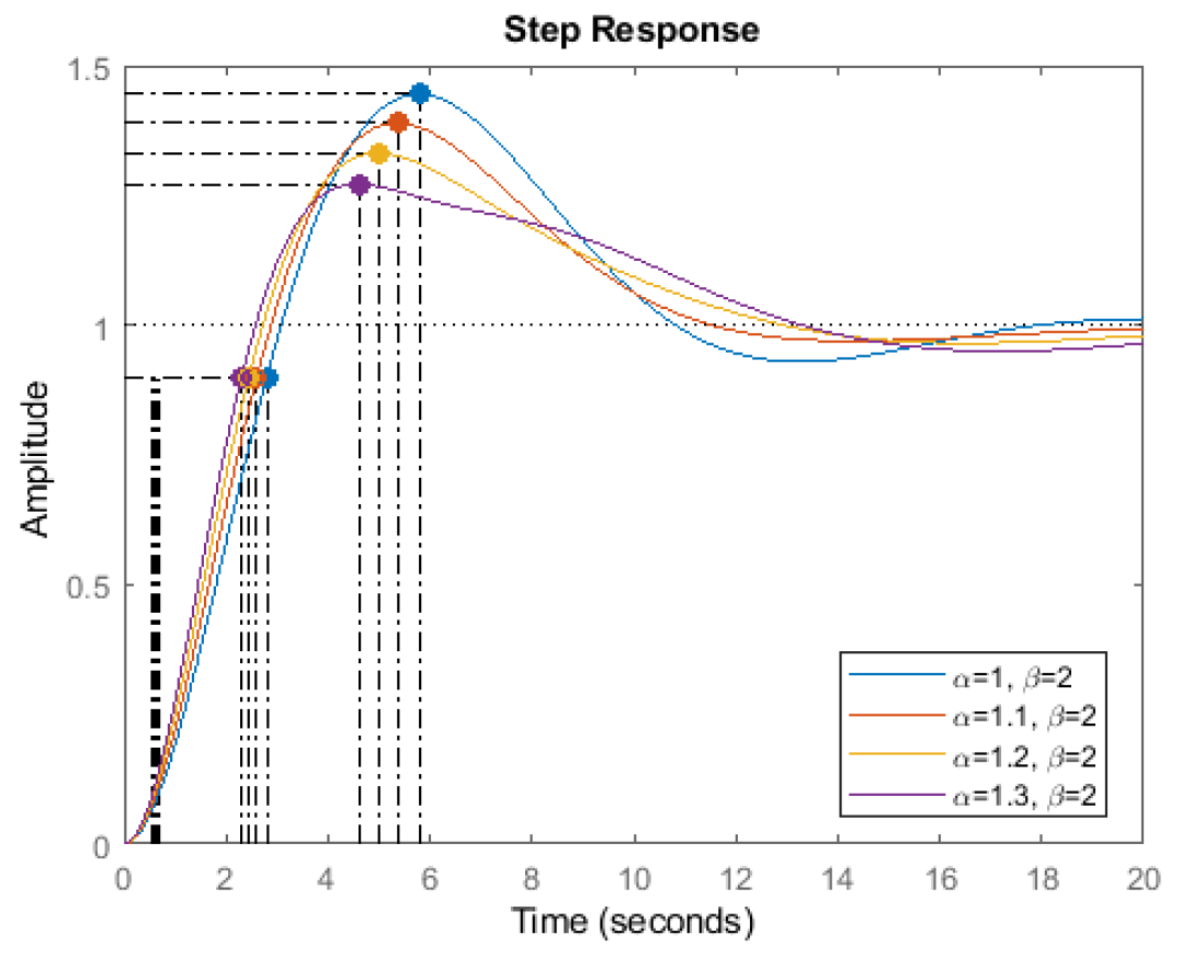
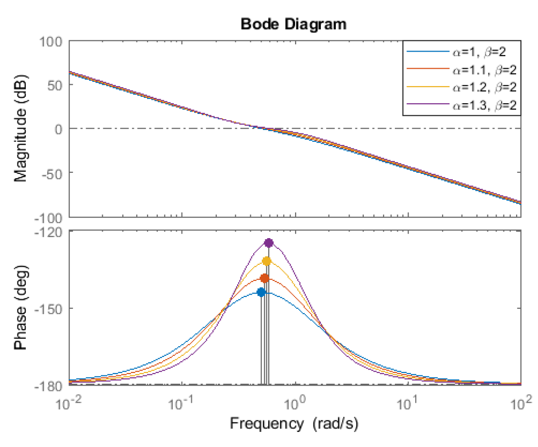
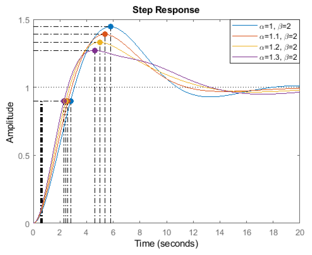
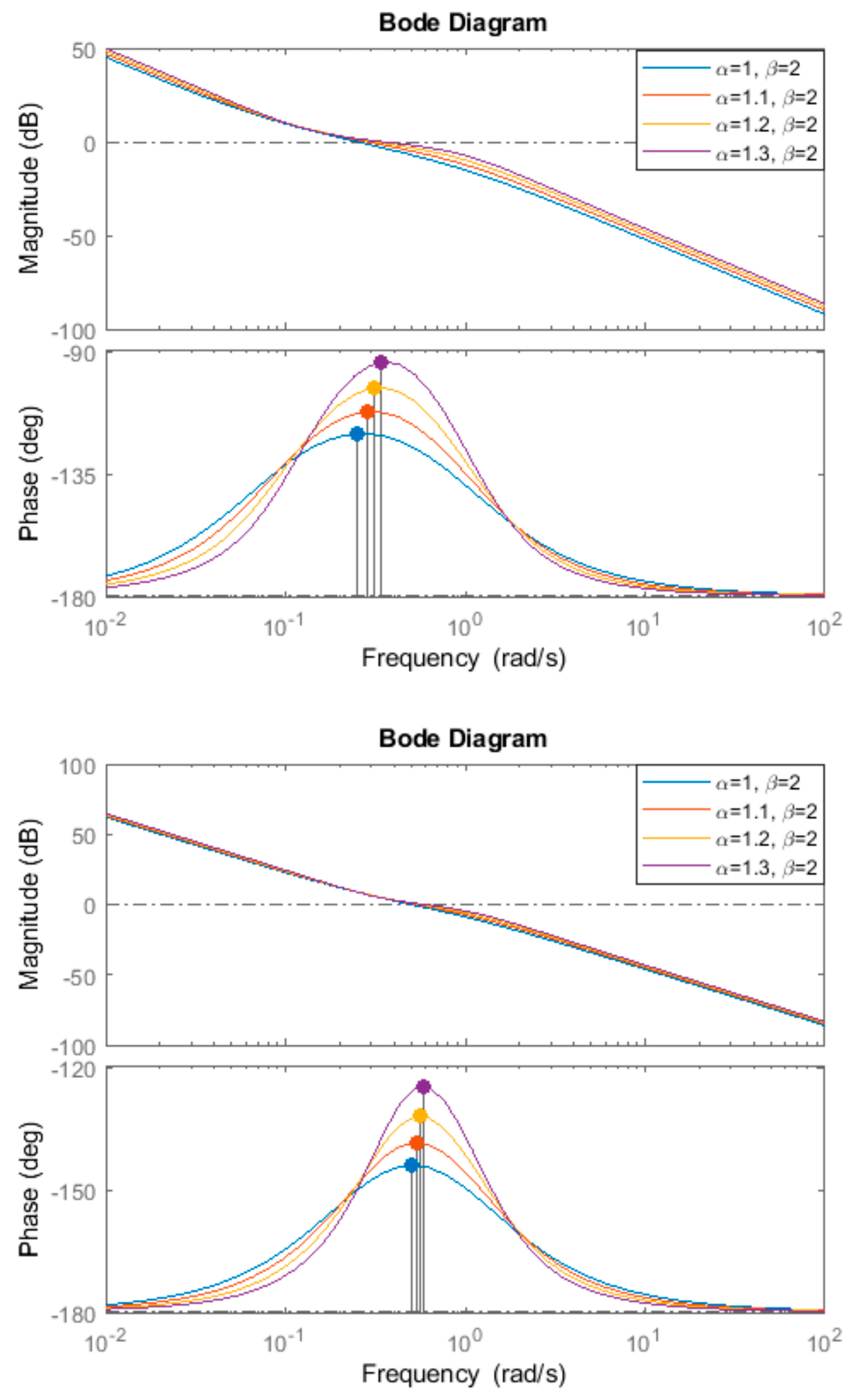
| β = 2 | 1 | 0.50 | 36.87 | 43.2 | 2.15 |
| 1.1 | 0.53 | 42.63 | 38.2 | 2.01 | |
| 1.2 | 0.56 | 49.29 | 33.0 | 1.95 | |
| 1.3 | 0.58 | 57.08 | 28.0 | 1.79 | |
| 1.4 | 0.60 | 66.38 | 23.4 | 1.69 | |
| 1.5 | 0.63 | 77.65 | 22.4 | 1.59 | |
| β = 3 | 1 | 0.33 | 50.90 | 24.9 | 3.39 |
| 1.1 | 0.36 | 58.00 | 18.5 | 3.26 | |
| 1.2 | 0.40 | 65.85 | 15.4 | 3.19 | |
| 1.3 | 0.42 | 74.62 | 15.0 | 2.62 | |
| 1.4 | 0.45 | 84.50 | 14.9 | 2.43 | |
| 1.5 | 0.48 | 95.76 | 14.8 | 2.22 | |
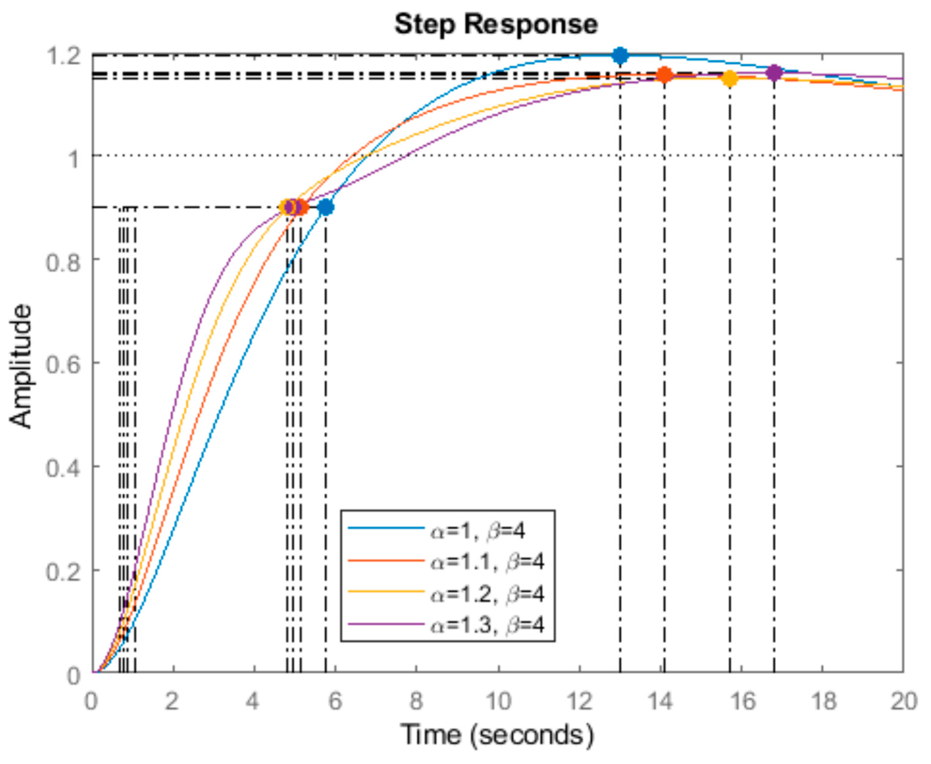
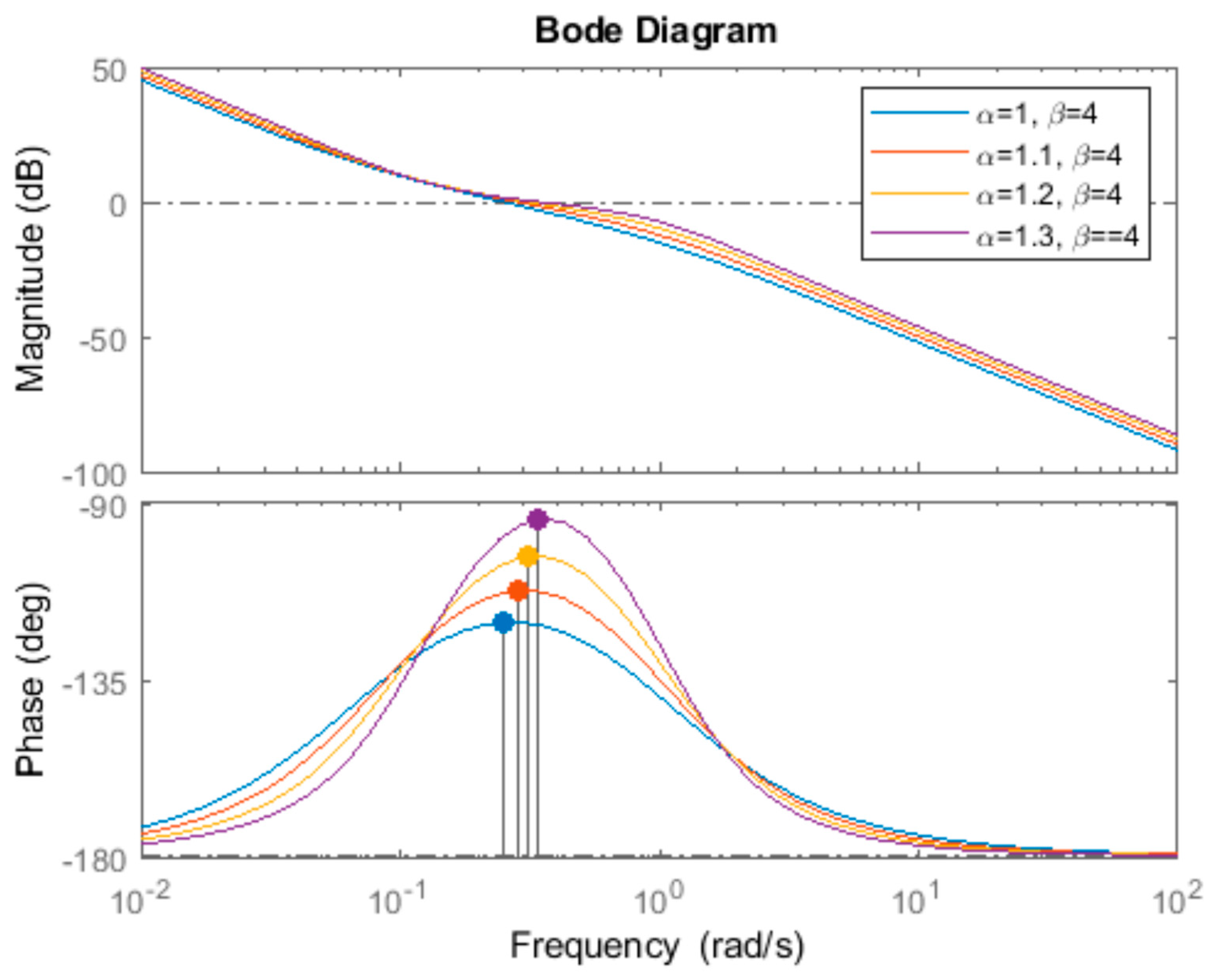
| β = 4 | 1 | 0.25 | 56.30 | 17.3 | 4.91 |
| 1.1 | 0.28 | 63.64 | 14.5 | 4.70 | |
| 1.2 | 0.31 | 71.59 | 13.3 | 4.58 | |
| 1.3 | 0.34 | 80.31 | 13.1 | 4.08 | |
| 1.4 | 0.37 | 89.96 | 13.0 | 3.74 | |
| 1.5 | 0.39 | 100.78 | 12.9 | 3.35 |
© 2019 by the author. Licensee MDPI, Basel, Switzerland. This article is an open access article distributed under the terms and conditions of the Creative Commons Attribution (CC BY) license (http://creativecommons.org/licenses/by/4.0/).
Share and Cite
Dulf, E.-H. Simplified Fractional Order Controller Design Algorithm. Mathematics 2019, 7, 1166. https://doi.org/10.3390/math7121166
Dulf E-H. Simplified Fractional Order Controller Design Algorithm. Mathematics. 2019; 7(12):1166. https://doi.org/10.3390/math7121166
Chicago/Turabian StyleDulf, Eva-Henrietta. 2019. "Simplified Fractional Order Controller Design Algorithm" Mathematics 7, no. 12: 1166. https://doi.org/10.3390/math7121166
APA StyleDulf, E.-H. (2019). Simplified Fractional Order Controller Design Algorithm. Mathematics, 7(12), 1166. https://doi.org/10.3390/math7121166