On Solving Modified Helmholtz Equation in Layered Materials Using the Multiple Source Meshfree Approach

Abstract

This paper presents a study for solving the modified Helmholtz equation in layered materials using the multiple source meshfree approach (MSMA). The key idea of the MSMA starts with the method of fundamental solutions (MFS) as well as the collocation Trefftz method (CTM). The multiple source collocation scheme in the MSMA stems from the MFS and the basis functions are formulated using the CTM. The solution of the modified Helmholtz equation is therefore approximated by the superposition theorem using particular nonsingular functions by means of multiple sources located within the domain. To deal with the two-dimensional modified Helmholtz equation in layered materials, the domain decomposition method was adopted. Numerical examples were carried out to validate the method. The results illustrate that the MSMA is relatively simple because it avoids a complicated procedure for finding the appropriate position of the sources. Additionally, the MSMA for solving the modified Helmholtz equation is advantageous because the source points can be collocated on or within the domain boundary and the results are not sensitive to the location of source points. Finally, compared with other methods, highly accurate solutions can be obtained using the proposed method.

1. Introduction

The solution of the modified Helmholtz equation plays a crucial role in the science and engineering fields, such as for boundary detection problems [1], water wave problems [2], Cauchy problems [3,4], diffusion equations [5], topological sensitivity analyses [6], and boundary value problems [7]. Over the past 10 years, conventional approaches have been widely adopted for solving the modified Helmholtz equation [8,9,10]. In contrast to the conventional approaches, several boundary collocation meshfree methods that have the basis functions satisfying the partial differential equation have also been proposed, for instance, the boundary knot method (BKM) [11,12], the boundary node method [13,14], the singular boundary method (SBM) [15,16,17], and the regularized meshless method [18,19]. In 2003, Chen and Hon [12] adopted the BKM to solve Helmholtz, modified Helmholtz, and the combination of diffusion and convection problems. The convergence of the BKM for the above equations was also investigated. Later, Chen et al. [15] applied the SBM to solve the modified Helmholtz equation. To examine the accuracy of the SBM, several wave numbers were considered in the numerical model [15]. For the modeling of Helmholtz-type equations in composite layered materials, Bin-Mohsin and Lesnic [20] adopted the method of fundamental solutions (MFS).

The MFS [21,22] is categorized into the indirect boundary element method or the boundary collocation meshfree approach, since only the boundary collocation points are used in the solution process. To avoid the singularity of the fundamental solutions, the MFS must collocate the source points outside the physical domain. Since it is a challenge to identify the location of source points, several attempts regarding this issue have been studied [23,24]. In 2007, Young et al. [25] proposed the modified MFS for finding the solution to the Laplace equation with an arbitrary domain. Later, Liu [26] adopted the multiple-length MFS (MLMFS) to investigate the appropriate placement of the sources for the Laplace equation. By using the MLMFS, the condition number can be reduced and the accuracy of the MLMFS may be increased. In recent years, Shigeta et al. [27] presented the multilayer method of fundamental solutions in conjunction with the weighted greedy QR decomposition (WGQRD) to solve the Laplace equation. As for the WGQRD, it can be used to find the necessary source points and unnecessary ones are removed in the numerical model.

Recently, Ku et al. [28] proposed a novel boundary-type meshfree method which is a hybrid of the MFS as well as the collocation Trefftz method (CTM). It adopts the collocation scheme from the MFS and the matrix form can be constructed in terms of superpositioning the nonsingular basis function from the CTM. This approach was then used for solving the Laplace-type subsurface flow problem. Xiao et al. [29] further applied the method to the problems of heat transfer in heterogeneous multilayer materials in two dimensions. Since the hybrid boundary-type meshless methods are only found to solve Laplace-type problems, it is especially interesting to explore this newly developed method for solving other non-Laplace problems. To the authors’ knowledge, pioneering work using the new boundary-type meshfree method to solve the modified Helmholtz equation in layered materials has not yet been proposed. We therefore propose a new boundary-type meshfree method using the basis functions based on the first-kind modified Bessel function capable of solving the two-dimensional modified Helmholtz equation over arbitrary geometries with doubly and multiply connected domains.

Starting from previous studies [28,29], we conducted pioneering work to solve the modified Helmholtz equation in layered materials. Since it is necessary to derive particular nonsingular basis functions for the two-dimensional modified Helmholtz equation, the specific method in this study is named the multiple source meshfree approach (MSMA). The key idea of the MSMA starts with the MFS and the CTM. The multiple source collocation scheme in the MSMA stems from the MFS, and the basis functions are formulated from the CTM. The solution of the modified Helmholtz equation is therefore approximated by the superposition theorem using particular nonsingular functions by means of multiple sources located within the domain. To deal with the two-dimensional modified Helmholtz equation in layered materials, the domain decomposition method (DDM) [30,31] was adopted. Numerical examples were carried out to validate the method.

The article is organized as follows: A brief introduction of the two-dimensional modified Helmholtz equation and the formulation of the MSMA considering the domain decomposition method are given in Section 2. In Section 3, several numerical examples are included to evaluate the accuracy of the proposed approach by comparing it with exact solutions. In Section 4, we discuss the research. Findings are summarized in Section 5.

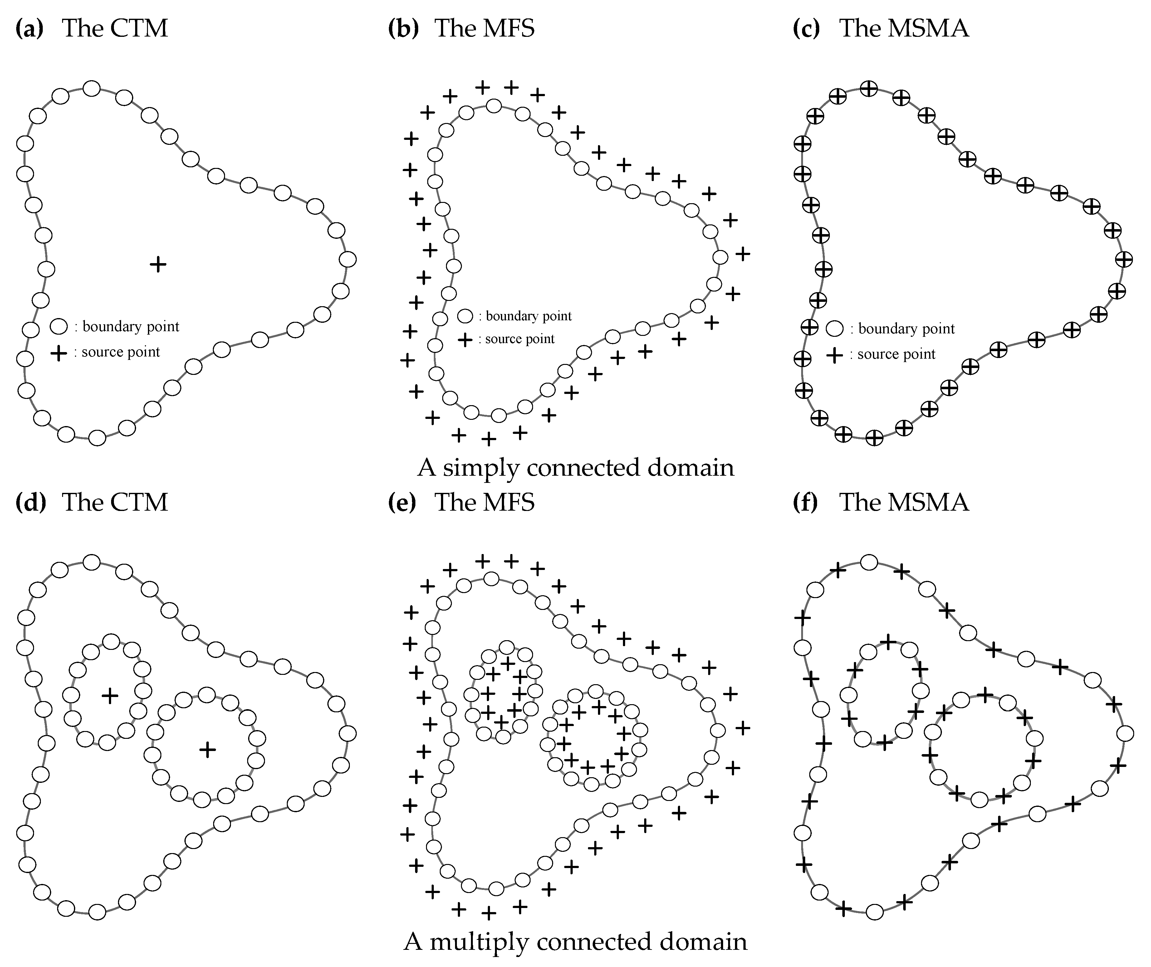
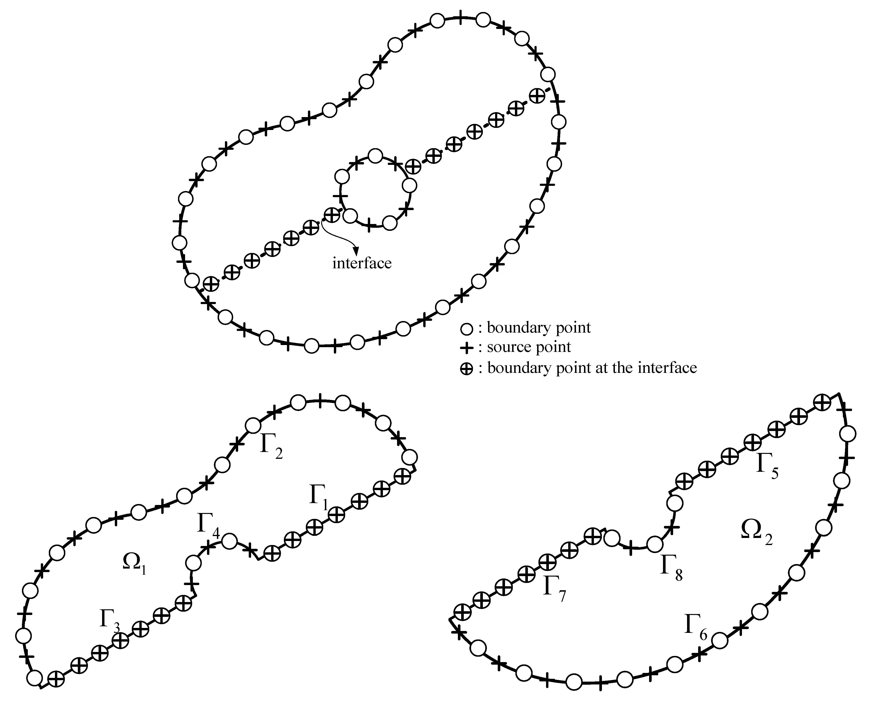
2. The Methodology

We consider a two-dimensional domain for the problem of interest in ${\Re }^2$ and assume that $\mathsf{\Omega }$ is enclosed by a boundary $\partial \mathsf{\Omega }=\Gamma$. The two-dimensional modified Helmholtz equation and the corresponding boundary conditions are stated as

$$({\nabla }^2-{\lambda }^2)u(x,y)=0,(x,y)\in \mathsf{\Omega }.$$

(1)

The Dirichlet and Neumann conditions are

$$u(x,y)=g(x,y)\mathrm{on}{\Gamma }_{\mathrm{D}}$$

(2)

$$\frac{\partial u(x,y)}{\partial n}=f(x,y)\mathrm{on}{\Gamma }_f$$

(3)

in which ${\Re }^2$ denotes the two-dimensional domain, ${\nabla }^2$ denotes the Laplacian, $u$ may represent temperature (or acoustic pressure), $\mathsf{\Omega }$ represents the domain of the problem, $\lambda$ is the wave number, $g$ and $f$ are the Dirichlet and Neumann boundary data, ${\Gamma }_{\mathrm{D}}$ and ${\Gamma }_f$ denote the boundaries where the Dirichlet and Neumann conditions are given, and $n$ represents the outward normal direction.

The idea of this study was originally motivated by the MFS and the CTM, in which the collocation scheme is from the MFS and the basis functions are from the Trefftz formulation. To elaborate the proposed MSMA, the collocation scheme is introduced first. Figure 1 demonstrates the collocation points for the MFS, CTM, and MSMA bounded by simply and multiply connected domains. As illustrated in Figure 1a, a source point is located within the physical boundary enclosed by a simply connected domain in the CTM. Instead of using just a source point, the concept of the MFS is to approximate the solutions via a fundamental solution by means of locating the sources away from the physical boundary, as illustrated in Figure 1b. As for the MSMA, the solution is approximated through the linear combination of the particular nonsingular functions in terms of multiple sources collocated within the physical boundary, as illustrated in Figure 1c. For a multiply connected domain, which includes more than one cavity, multiple sources are placed within the physical boundary. The collocation scheme of the sources is demonstrated in Figure 1d–f for the CTM, MFS, and MSMA. From Figure 1, it is obvious that the proposed MSMA is advantageous because we may place the source and boundary points at the same position. Also, unlike the MFS, the source points can be placed at any position and are not sensitive to the results.

In the MSMA, the solution of the modified Helmholtz equation is approximated by the superposition theorem using nonsingular general solutions by means of multiple sources. Numerical solutions of the modified Helmholtz equation in two dimensions may be expressed as the combination of nonsingular general solutions. We may rewrite the two-dimensional modified Helmholtz equation in the polar coordinate as follows:

$$\frac{{\partial }^{2}u}{\partial r^2}+\frac{1}{r}\frac{\partial u}{\partial r}+\frac{1}{r^2}\frac{{\partial }^{2}u}{\partial {\theta }^2}-{\lambda }^{2}u=0$$

(4)

where $r$ represents the radial coordinate and $\theta$ is the angular coordinate. For Equation (4), particular nonsingular functions can be derived using the separation of variables. Since the solutions are expressed as the linear superposition of the nonsingular functions, we may obtain the numerical solution of the two-dimensional modified Helmholtz equation represented by the linear superposition of the nonsingular basis functions:

$$u(\mathbf{x})\approx {\displaystyle \sum _{j=1}^S{\displaystyle \sum _{k=1}^P{\mathbf{a}}_{j,k}{\mathbf{H}}_{j,k}}(\mathbf{x},{\mathbf{y}}_j)}$$

(5)

in which $\mathbf{x}\in \mathsf{\Omega }$, ${\mathbf{y}}_j$ is the source point, ${\mathbf{a}}_{j,k}$ denotes a vector of unknown coefficients, $S$ denotes the source point number, and $P$ represents the terms of the particular solutions. The particular solutions [4], ${\mathbf{H}}_{j,k}(\mathbf{x},{\mathbf{y}}_j)$, can be derived using the separation of variables for the two-dimensional modified Helmholtz equation in a simply connected domain given by

$${\mathbf{H}}_{j,k}(\mathbf{x},{\mathbf{y}}_j)={[\begin{array}{cc}{\mathrm{I}}_k(\lambda {\rho }_j)\sin (k{\theta }_j)& {\mathrm{I}}_k(\lambda {\rho }_j)\cos (k{\theta }_j)\end{array}]}^{\mathrm{T}}$$

(6)

where ${\mathrm{I}}_k$ is the modified Bessel function of order $k$ for the first kind; ${\rho }_j$ denotes the distance between the boundary collocation point and the source point, ${\rho }_j=\left|\mathbf{x}-{\mathbf{y}}_j\right|$; and ${\theta }_j$ is the angle of the boundary point and the source point. For the Dirichlet boundary condition, we have

$$u({\mathbf{x}}_l)\approx {\displaystyle \sum _{j=1}^S{\displaystyle \sum _{k=1}^P{\mathbf{a}}_{j,k}{\mathbf{H}}_{j,k}}({\mathbf{x}}_l,{\mathbf{y}}_j)}=g({\mathbf{x}}_l)$$

(7)

in which $l=1,\dots ,Q$, $Q$ represents the boundary point number, and $g({\mathbf{x}}_l)$ represents the Dirichlet boundary data given on the boundary points. From Equation (3), the boundary of the Neumann condition is rewritten as

$$\frac{\partial u({\mathbf{x}}_l)}{\partial n}=(\frac{\partial u({\mathbf{x}}_l)}{\partial \rho }\frac{\partial \rho }{\partial x}+\frac{\partial u({\mathbf{x}}_l)}{\partial \theta }\frac{\partial \theta }{\partial x})n_x+(\frac{\partial u({\mathbf{x}}_l)}{\partial \rho }\frac{\partial \rho }{\partial y}+\frac{\partial u({\mathbf{x}}_l)}{\partial \theta }\frac{\partial \theta }{\partial y})n_y$$

(8)

where $n_x$ and $n_y$ at ${\mathbf{x}}_l$ denote the outward normal direction vector. Using Equation (5), the derivatives of $\partial u/\partial \rho$ and $\partial u/\partial \theta$ are given by

$$\frac{\partial u({\mathbf{x}}_l)}{\partial \rho }={\displaystyle \sum _{j=1}^S{\displaystyle \sum _{k=1}^P{\mathbf{a}}_{j,k}{[\begin{array}{cc}\lambda {\mathrm{I}}_{(k+1)}(\lambda {\rho }_j)+(\frac{k}{{\rho }_j}){\mathrm{I}}_k(\lambda {\rho }_j)\sin (k{\theta }_j)& \lambda {\mathrm{I}}_{(k+1)}(\lambda {\rho }_j)+(\frac{k}{{\rho }_j}){\mathrm{I}}_k(\lambda {\rho }_j)\cos (k{\theta }_j)\end{array}]}^{\mathrm{T}}}}$$

(9)

$$\frac{\partial u({\mathbf{x}}_l)}{\partial \theta }={\displaystyle \sum _{j=1}^S{\displaystyle \sum _{k=1}^P{\mathbf{a}}_{j,k}{[\begin{array}{cc}k{\mathrm{I}}_k(\lambda {\rho }_j)\cos (k{\theta }_j)& -k{\mathrm{I}}_k(\lambda {\rho }_j)\sin (k{\theta }_j)\end{array}]}^{\mathrm{T}}}}.$$

(10)

Substituting Equations (9) and (10) into Equation (8), the following equation is listed below:

$$\frac{\partial u({\mathbf{x}}_l)}{\partial n}={\displaystyle \sum _{j=1}^S{\displaystyle \sum _{k=1}^P{\mathbf{a}}_{j,k}{[\begin{array}{cc}\partial ({\mathrm{I}}_k(\lambda {\rho }_j)\sin (k{\theta }_j))/\partial n& \partial ({\mathrm{I}}_k(\lambda {\rho }_j)\cos (k{\theta }_j))/\partial n\end{array}]}^{\mathrm{T}}}}$$

(11)

where

$$\frac{\partial ({\mathrm{I}}_k(\lambda {\rho }_j)\sin (k{\theta }_j))}{\partial n}={\displaystyle \sum _{j=1}^S{\displaystyle \sum _{k=1}^P\begin{array}{c}[\lambda {\mathrm{I}}_{(k+1)}(\lambda {\rho }_j)+(\frac{k}{{\rho }_j}){\mathrm{I}}_k(\lambda {\rho }_j)\sin (k{\theta }_j)\cos {\theta }_j-k{\mathrm{I}}_k(\lambda {\rho }_j)\cos (k{\theta }_j)(\frac{\sin {\theta }_j}{{\rho }_j})]n_x\\ +[\lambda {\mathrm{I}}_{(k+1)}(\lambda {\rho }_j)+(\frac{k}{{\rho }_j}){\mathrm{I}}_k(\lambda {\rho }_j)\sin (k{\theta }_j)\sin {\theta }_j+k{\mathrm{I}}_k(\lambda {\rho }_j)\cos (k{\theta }_j)(\frac{\cos {\theta }_j}{{\rho }_j})]n_y\end{array}}},$$

(12)

$$\frac{\partial ({\mathrm{I}}_k(\lambda {\rho }_j)\cos (k{\theta }_j))}{\partial n}={\displaystyle \sum _{j=1}^S{\displaystyle \sum _{k=1}^P\begin{array}{c}[\lambda {\mathrm{I}}_{(k+1)}(\lambda {\rho }_j)+(\frac{k}{{\rho }_j}){\mathrm{I}}_k(\lambda {\rho }_j)\cos (k{\theta }_j)\cos {\theta }_j+k{\mathrm{I}}_k(\lambda {\rho }_j)\sin (k{\theta }_j)(\frac{\sin {\theta }_j}{{\rho }_j})]n_x\\ +[\lambda {\mathrm{I}}_{(k+1)}(\lambda {\rho }_j)+(\frac{k}{{\rho }_j}){\mathrm{I}}_k(\lambda {\rho }_j)\cos (k{\theta }_j)\sin {\theta }_j-k{\mathrm{I}}_k(\lambda {\rho }_j)\sin (k{\theta }_j)(\frac{\cos {\theta }_j}{{\rho }_j})]n_y\end{array}}},$$

(13)

Neumann boundary data are also imposed on the domain boundary using Equation (8):

$$\frac{\partial u({\mathbf{x}}_l)}{\partial n}\approx {\displaystyle \sum _{j=1}^S{\displaystyle \sum _{k=1}^P{\mathbf{a}}_{j,k}{[\begin{array}{cc}\partial ({\mathrm{I}}_k(\lambda {\rho }_j)\sin (k{\theta }_j))/\partial n& \partial ({\mathrm{I}}_k(\lambda {\rho }_j)\cos (k{\theta }_j))/\partial n\end{array}]}^{\mathrm{T}}}}=f({\mathbf{x}}_l)$$

(14)

where $l=1,\dots ,Q$, and $f({\mathbf{x}}_l)$ represents the Neumann boundary data given on the boundary points. Using Equations (7) and (14), the following equation can be obtained as

$$\mathbf{A}\mathsf{\alpha }=\mathbf{b}$$

(15)

where $\mathbf{A}=\left[\begin{array}{ccccc}{\mathrm{I}}_1(\lambda {\rho }_1)\sin ({\theta }_1)& {\mathrm{I}}_1(\lambda {\rho }_1)\cos ({\theta }_1)& \cdots & {\mathrm{I}}_k(\lambda {\rho }_1)\sin (k{\theta }_1)& {\mathrm{I}}_k(\lambda {\rho }_1)\cos (k{\theta }_1)\\ {\mathrm{I}}_1(\lambda {\rho }_2)\sin ({\theta }_2)& {\mathrm{I}}_1(\lambda {\rho }_2)\cos ({\theta }_2)& \cdots & {\mathrm{I}}_k(\lambda {\rho }_2)\sin (k{\theta }_2)& {\mathrm{I}}_k(\lambda {\rho }_2)\cos (k{\theta }_2)\\ ⋮& ⋮& \ddots & ⋮& ⋮\\ {\mathrm{I}}_1(\lambda {\rho }_c)\sin ({\theta }_c)& {\mathrm{I}}_1(\lambda {\rho }_c)\cos ({\theta }_c)& \cdots & {\mathrm{I}}_k(\lambda {\rho }_c)\sin (k{\theta }_c)& {\mathrm{I}}_k(\lambda {\rho }_c)\cos (k{\theta }_c)\\ {\mathrm{N}}_{j,k=1}^{\mathrm{I}}& {\mathrm{N}}_{j,k=1}^{\mathrm{II}}& \cdots & {\mathrm{N}}_{j,k=P}^{\mathrm{I}}& {\mathrm{N}}_{j,k=P}^{\mathrm{I}\mathrm{I}}\\ {\mathrm{N}}_{j,k=1}^{\mathrm{I}}& {\mathrm{N}}_{j,k=1}^{\mathrm{I}\mathrm{I}}& \cdots & {\mathrm{N}}_{j,k=P}^{\mathrm{I}}& {\mathrm{N}}_{j,k=P}^{\mathrm{I}\mathrm{I}}\\ ⋮& ⋮& \ddots & ⋮& ⋮\\ {\mathrm{N}}_{j,k=1}^{\mathrm{I}}& {\mathrm{N}}_{j,k=1}^{\mathrm{I}\mathrm{I}}& \cdots & {\mathrm{N}}_{j,k=P}^{\mathrm{I}}& {\mathrm{N}}_{j,k=P}^{\mathrm{I}\mathrm{I}}\end{array}\right],$

$$\mathsf{\alpha }={\left[\begin{array}{cccccccc}{a}_1& a_2& a_3& \dots & \dots & a_{m-2}& a_{m-1}& a_m\end{array}\right]}^{\mathrm{T}},\mathbf{b}={\left[\begin{array}{cccccccc}{g}_1& g_2& \dots & g_c& f_1& f_2& \dots & f_d\end{array}\right]}^{\mathrm{T}},$$

(16)

and

$${\mathrm{N}}_{j,k}^{\mathrm{I}}={\displaystyle \sum _{j=1}^{\mathrm{S}}{\displaystyle \sum _{k=1}^{\mathrm{P}}\begin{array}{c}[\lambda {\mathrm{I}}_{(k+1)}(\lambda {\rho }_j)+(k/{\rho }_j){\mathrm{I}}_k(\lambda {\rho }_j)\sin (k{\theta }_j)\cos {\theta }_j-k{\mathrm{I}}_k(\lambda {\rho }_j)\cos (k{\theta }_j)(\sin {\theta }_j/{\rho }_j)]n_x\\ +[\lambda {\mathrm{I}}_{(k+1)}(\lambda {\rho }_j)+(k/{\rho }_j){\mathrm{I}}_k(\lambda {\rho }_j)\sin (k{\theta }_j)\sin {\theta }_j+k{\mathrm{I}}_k(\lambda {\rho }_j)\cos (k{\theta }_j)(\cos {\theta }_j/{\rho }_j)]n_y\end{array}}}$$

(17)

$${\mathrm{N}}_{j,k}^{\mathrm{I}\mathrm{I}}={\displaystyle \sum _{j=1}^{\mathrm{S}}{\displaystyle \sum _{k=1}^{\mathrm{P}}\begin{array}{c}[\lambda {\mathrm{I}}_{(k+1)}(\lambda {\rho }_j)+(k/{\rho }_j){\mathrm{I}}_k(\lambda {\rho }_j)\cos (k{\theta }_j)\cos {\theta }_j+k{\mathrm{I}}_k(\lambda {\rho }_j)\sin (k{\theta }_j)(\sin {\theta }_j/{\rho }_j)]n_x\\ +[\lambda {\mathrm{I}}_{(k+1)}(\lambda {\rho }_j)+(k/{\rho }_j){\mathrm{I}}_k(\lambda {\rho }_j)\cos (k{\theta }_j)\sin {\theta }_j-k{\mathrm{I}}_k(\lambda {\rho }_j)\sin (k{\theta }_j)(\cos {\theta }_j/{\rho }_j)]n_y\end{array}}}.$$

(18)

In the preceding equations, $\mathbf{A}$ is a $Q\times S$ matrix, $S$ represents the source point number, $\mathsf{\alpha }$ represents a vector with the size of $S\times 1$ for unknown coefficients, $\mathbf{b}$ denotes a vector with the size of $Q\times 1$ for boundary values, $c$ and $d$ represent the boundary point number for Dirichlet and Neumann boundary data, respectively, $a_1,a_2,\dots ,a_m$ are unknown coefficients to be determined, and $g_1,g_2,\dots ,g_c$ and $f_1,f_2,\dots ,f_d$ denote the Dirichlet and Neumann boundary data, respectively.

To deal with the two-dimensional modified Helmholtz equation in layered materials, the DDM [30,31] was adopted. It should be noted that the DDM was also used to deal with the problems bounded by doubly and multiply connected domains in this study because the proposed MSMA approximates the solution of the two-dimensional modified Helmholtz equation as the combination of only particular nonsingular basis functions.

Unlike the CTM or the MFS, the MSMA does not consider the negative basis functions or the so-called singular basis functions in the proposed method. As a result, we are not able to tackle the singular solution in the cavity by using only the nonsingular basis functions. It is therefore necessary to split the domain into several simply connected subregions, such that we may guarantee subregions existing only in a nonsingular solution.

In the DDM, the physical boundary is split into several simply connected subregions which are connected at the interface between two consecutive subregions, as depicted in Figure 2. At the interface, the overspecified boundary data need to be satisfied. A doubly connected domain, $\mathsf{\Omega }$, is split into two subregions, ${\mathsf{\Omega }}_1$ and ${\mathsf{\Omega }}_2$. For the subregions, we have ${\Gamma }_1$, ${\Gamma }_2$, …, and ${\Gamma }_8$ sub-boundaries, in which ${\mathsf{\Omega }}_1$ is composed of ${\Gamma }_1$, ${\Gamma }_2$, ${\Gamma }_3$, and ${\Gamma }_4$ and ${\mathsf{\Omega }}_2$ is composed of ${\Gamma }_5$, ${\Gamma }_6$, ${\Gamma }_7$, and ${\Gamma }_8$. To connect ${\mathsf{\Omega }}_1$ and ${\mathsf{\Omega }}_2$, we may use both the Dirichlet and Neumann boundary conditions to satisfy the continuity condition on the interface. The form of the continuity equations is described as follows:

$${u|}_{{\Gamma }_1}={u|}_{{\Gamma }_5},{\frac{\partial u}{\partial n}|}_{{\Gamma }_1}={\frac{\partial u}{\partial n}|}_{{\Gamma }_5},{u|}_{{\Gamma }_3}={u|}_{{\Gamma }_7},{\frac{\partial u}{\partial n}|}_{{\Gamma }_3}={\frac{\partial u}{\partial n}|}_{{\Gamma }_7}.$$

(19)

Using the DDM, we can obtain the matrix form, which is expressed as follows:

$${\mathbf{A}}_{\mathrm{D}}{\mathsf{\alpha }}_{\mathrm{D}}={\mathbf{b}}_{\mathrm{D}}$$

(20)

$${\mathbf{A}}_{\mathrm{D}}=\left[\begin{array}{cc}{\mathbf{A}}_{{\mathsf{\Omega }}_1}& {\mathbf{0}}_{{\mathsf{\Omega }}_2}\\ {{\mathbf{A}}_{\mathrm{I}}|}_{{\Gamma }_1,{\Gamma }_3}& {{\mathbf{A}}_{\mathrm{I}}|}_{{\Gamma }_5,{\Gamma }_7}\\ {\mathbf{0}}_{{\mathsf{\Omega }}_1}& {\mathbf{A}}_{{\mathsf{\Omega }}_2}\end{array}\right],{\mathsf{\alpha }}_{\mathrm{D}}=\left[\begin{array}{c}{\mathsf{\alpha }}_{{\mathsf{\Omega }}_1}\\ {\mathsf{\alpha }}_{{\mathsf{\Omega }}_2}\end{array}\right],{\mathbf{b}}_{\mathrm{D}}=\left[\begin{array}{c}{\mathbf{b}}_{{\mathsf{\Omega }}_1}\\ {\mathbf{b}}_{\mathrm{I}}\\ {\mathbf{b}}_{{\mathsf{\Omega }}_2}\end{array}\right]$$

(21)

where ${\mathbf{A}}_{{\mathsf{\Omega }}_1}$ and ${\mathbf{A}}_{{\mathsf{\Omega }}_2}$ are the matrix with the size of $m_1\times n_1$ and $m_2\times n_2$ for ${\mathsf{\Omega }}_1$ and ${\mathsf{\Omega }}_2$; $m_1$ and $m_2$ are the boundary collocation points for ${\mathsf{\Omega }}_1$ and ${\mathsf{\Omega }}_2$, respectively; and $n_1$ and $n_2$ are the terms of the particular solutions for ${\mathsf{\Omega }}_1$ and ${\mathsf{\Omega }}_2$, respectively. At the interface, ${{\mathbf{A}}_{\mathrm{I}}|}_{{\Gamma }_1,{\Gamma }_3}$ has the size of $m_I\times n_1$ for the boundary ${\Gamma }_1$ and ${\Gamma }_3$, and ${{\mathbf{A}}_{\mathrm{I}}|}_{{\Gamma }_5,{\Gamma }_7}$ has the size of $m_I\times n_2$ for the boundary ${\Gamma }_5$ and ${\Gamma }_7$. $m_I$ represents the boundary point number at the interface. ${\mathbf{0}}_{{\mathsf{\Omega }}_1}$ and ${\mathbf{0}}_{{\mathsf{\Omega }}_2}$ are vectors for which all values are zero with the size of $m_2\times n_1$ and $m_1\times n_2$, respectively. ${\mathsf{\alpha }}_{{\mathsf{\Omega }}_1}$ denotes a $n_1\times 1$ vector of unknown coefficients of ${\mathsf{\Omega }}_1$, ${\mathsf{\alpha }}_{{\mathsf{\Omega }}_2}$ denotes a $n_2\times 1$ vector of unknown coefficients of ${\mathsf{\Omega }}_2$. ${\mathbf{b}}_{\mathrm{I}}$ is the vector with the size of $m_I\times 1$ at the interface, ${\mathbf{b}}_{\mathrm{I}}=\begin{array}{cc}[{\mathbf{0}}_{\mathrm{g}}& {\mathbf{0}}_{\mathrm{f}}\end{array}{]}^{\mathrm{T}}$, and 0_g and 0_f are vectors for which all values are zero. Solving the matrix form expressed in Equation (20), unknown coefficients ${\mathbf{b}}_{{\mathsf{\Omega }}_1}$ and ${\mathbf{b}}_{{\mathsf{\Omega }}_2}$ for subdomains ${\mathsf{\Omega }}_1$ and ${\mathsf{\Omega }}_2$ can then be determined.

3. Numerical Examples

To validate the MSMA for solving the modified Helmholtz equation, six examples were conducted to verify the proposed meshfree approach. The absolute error and relative root-mean-square error were used to evaluate the accuracy of the numerical solution as follows:

$$\mathrm{Absolute}\mathrm{error}=\left|u_{ana}({\mathbf{x}}_i)-u_{nu}({\mathbf{x}}_i)\right|,$$

(22)

$$\mathrm{Relative}\mathrm{root}-\mathrm{mean}-\mathrm{square}\mathrm{error}=\sqrt{\frac{1}{nt}{\displaystyle \sum _{i=1}^{nt}{(u_{nu}({\mathbf{x}}_i)-u_{ana}({\mathbf{x}}_i))}^2}}/\sqrt{\frac{1}{nt}{\displaystyle \sum _{i=1}^{nt}{u}_{ana}{}^2(x_i)}}$$

(23)

where $nt$ is the number of inner points in the domain, and $u_{nu}({\mathbf{x}}_i)$ and $u_{nu}({\mathbf{x}}_i)$ are the analytical and numerical solutions at ${\mathbf{x}}_i$, respectively.

3.1. Modeling of Modified Helmholtz Equation Bounded by a Simply Connected Region

This example is the modeling of the modified Helmholtz equation bounded by a simply connected region with a gear-shaped domain, as depicted in Figure 3. The shape parameter of the physical boundary is given by

$$\partial \mathsf{\Omega }=\left\{(x,y)|x=\rho (\theta )\cos (\sigma (\theta )),y=\rho (\theta )\sin (\sigma (\theta ))\right\},$$

(24)

where $\rho (\theta )=0.2\left(2+0.5\sin (7\theta )\right)$, $\sigma (\theta )=\theta +0.5\sin (7\theta )$, and $0\le \theta \le 2\pi$.

We consider the following exact solution:

$$u={\mathrm{e}}^{\lambda /\sqrt{2}(x+y)}.$$

(25)

In this case, the Dirichlet and Neumann boundary data are imposed using the exact solution. The wave number $\lambda$ is set as $\sqrt{2}$. Figure 3 illustrates the maximum absolute error (MAE) versus the terms of the particular solutions, $k$. The MSMA can obtain highly accurate results in the order of ${10}^{-11}$ while $k=15$. Figure 4 demonstrates the relationship of the MAE with the source point number. When the source points number is more than 100, the proposed MSMA can obtain accurate results with the order of ${10}^{-10}$. As shown in Figure 5, we found that the accuracy of the results decreased with the increase of the wave number $\lambda$. To obtain the MAE, 1211 inner points were uniformly located within the domain. Figure 6 shows the comparison of the numerical and analytical solutions. The results demonstrate that the solutions of the MSMA agree very well with the exact solution.

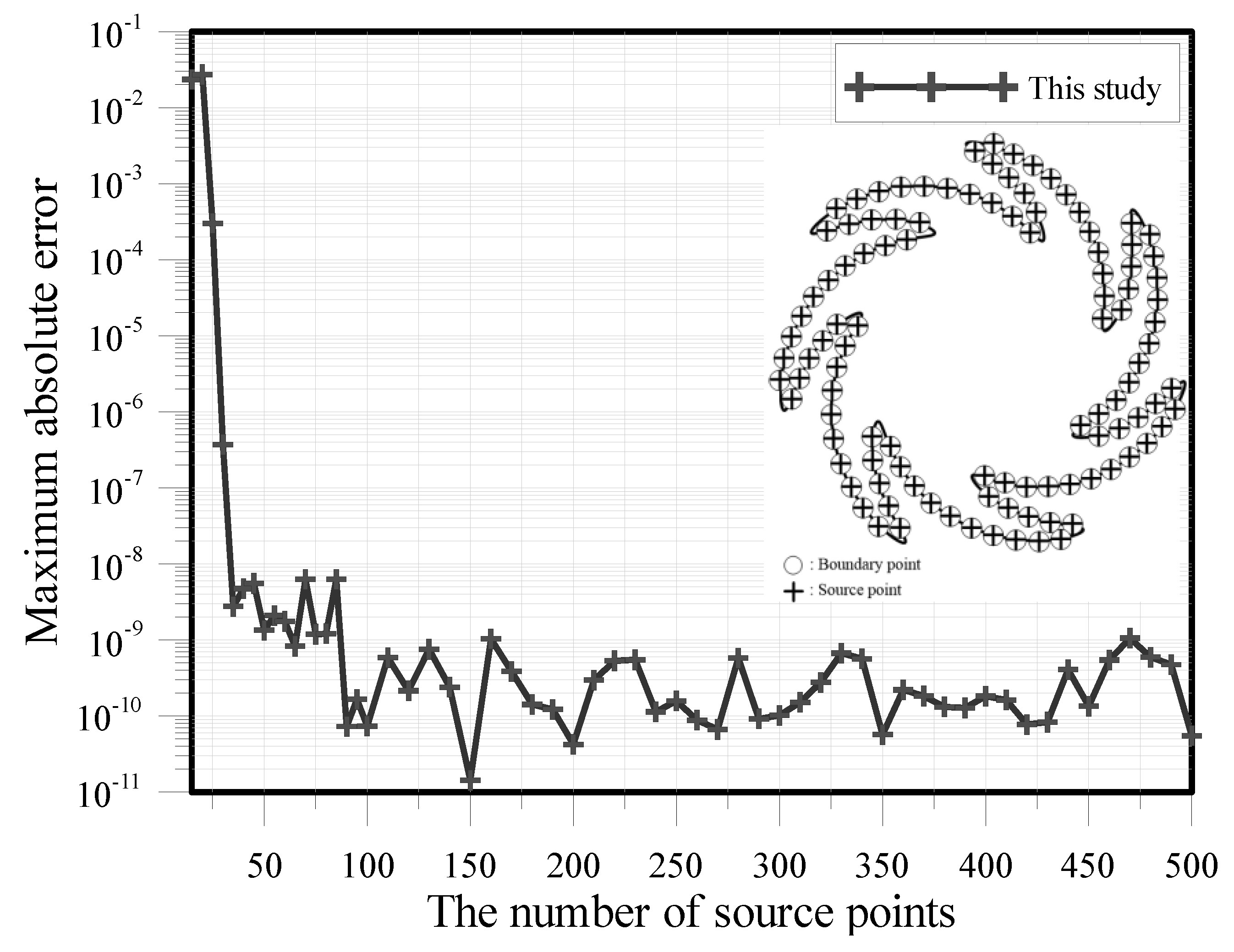
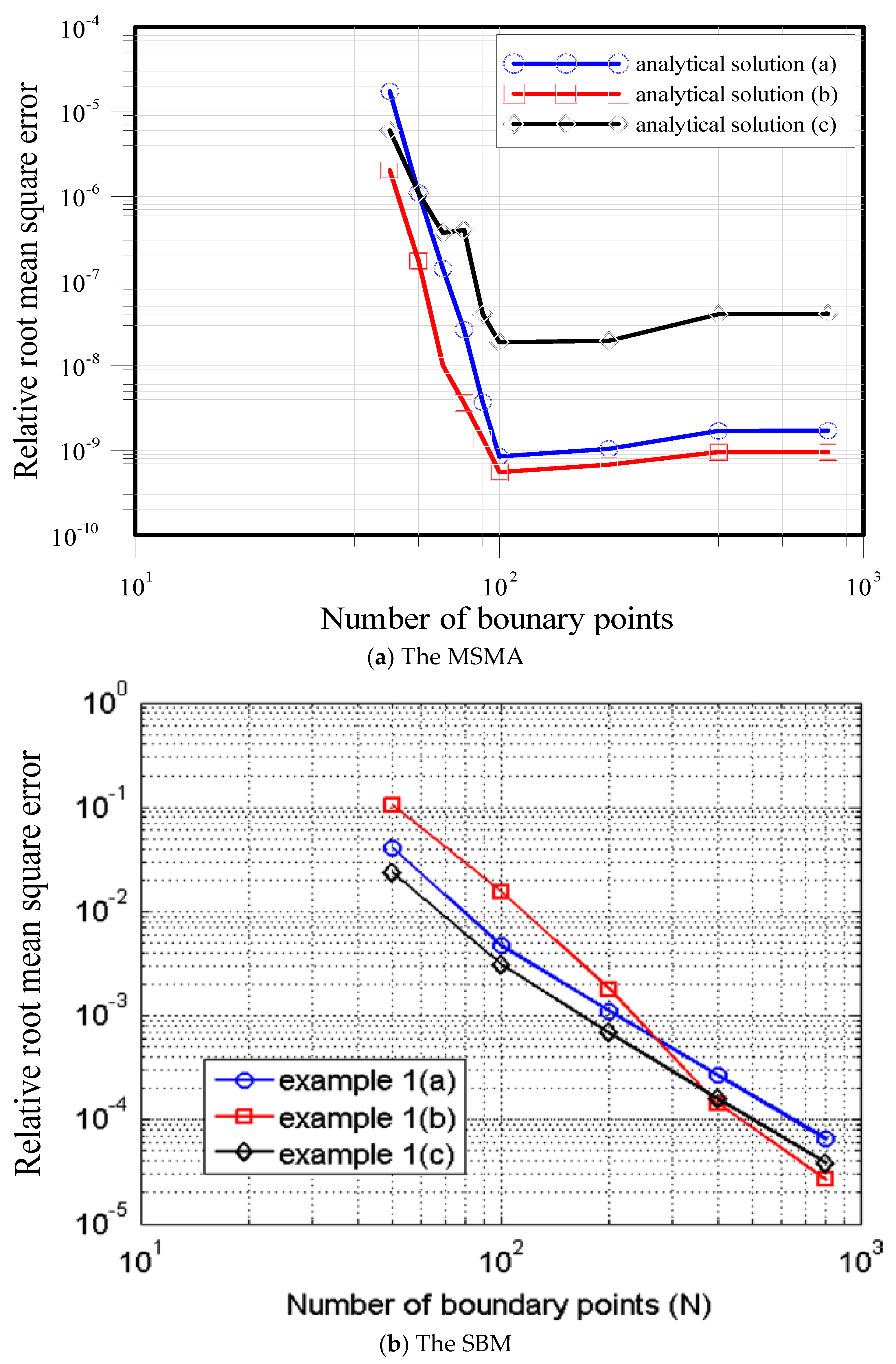
3.2. Accuracy Comparison of the Proposed Method

The second case is the modeling of the modified Helmholtz equation bounded by an amoeba-shaped boundary, as illustrated in Figure 7. In this example, the results computed by MSMA were compared with those from the SBM [15]. The shape parameter of the irregular physical boundary is described by

$$\partial \mathsf{\Omega }=\left\{(x,y)|x=\rho (\theta )\cos (\theta ),y=\rho (\theta )\sin (\theta )\right\},$$

(26)

in which $\rho ={\mathrm{e}}^{{(\sin \theta \sin 2\theta )}^2}+{\mathrm{e}}^{{(\cos \theta \cos 2\theta )}^2}$, and $0\le \theta \le 2\pi$.

Three different exact solutions can be found as follows:

$$u={\mathrm{e}}^{\lambda x},$$

(27)

$$u={\mathrm{e}}^{(\sqrt{2}\lambda /2)(x-y)},$$

(28)

$$u={\mathrm{e}}^{(\lambda /2)(x+\sqrt{3}y)}.$$

(29)

In the numerical implementation, the terms of the particular solutions, $k$, was 15. The Dirichlet boundary data were imposed on the domain boundary using three different analytical solutions, as depicted in Equations (27)–(29). The wave number $\lambda$ was set as $\pi$. The computed results using the MSMA were compared with the SBM [15]. We obtained highly accurate numerical solutions while the boundary and source point number was greater than 100, as shown in Figure 8a. Compared with the results using the SBM [15] as shown in Figure 8b, we found that the accuracy of the MSMA was much more accurate than the SBM. Figure 9a shows the accuracy for the relative root-mean-square error versus the wave number. It was found that the accuracy of the increased wave number may decrease the accuracy of the computed results. Figure 9b shows the relative root-mean-square error versus the wave number computed by the SBM [15]. Figure 9 shows that the accuracy of the MSMA is better than that from the SBM.

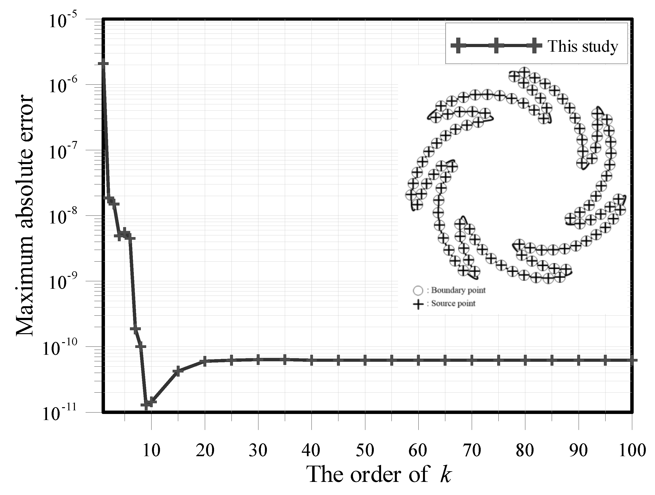
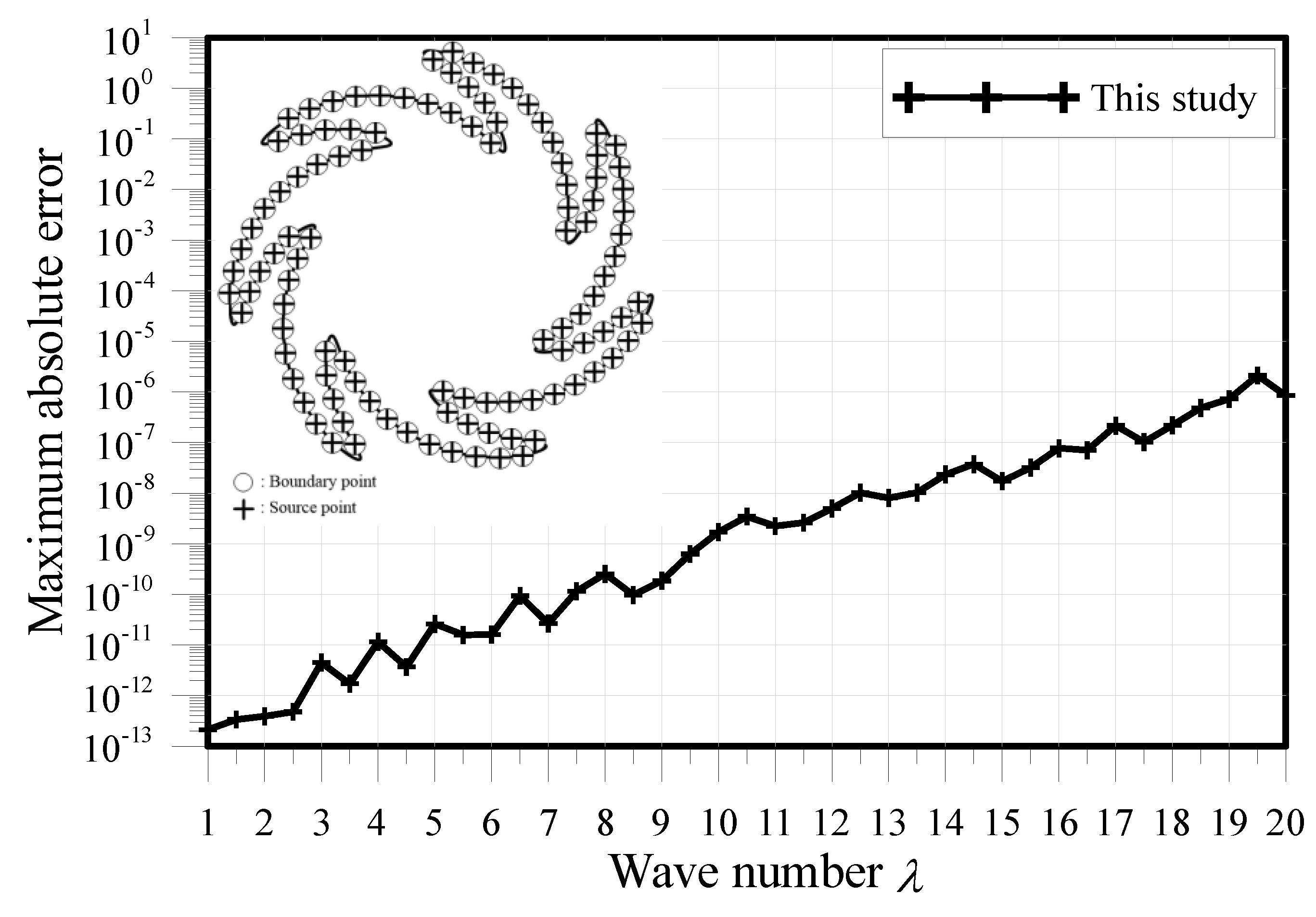
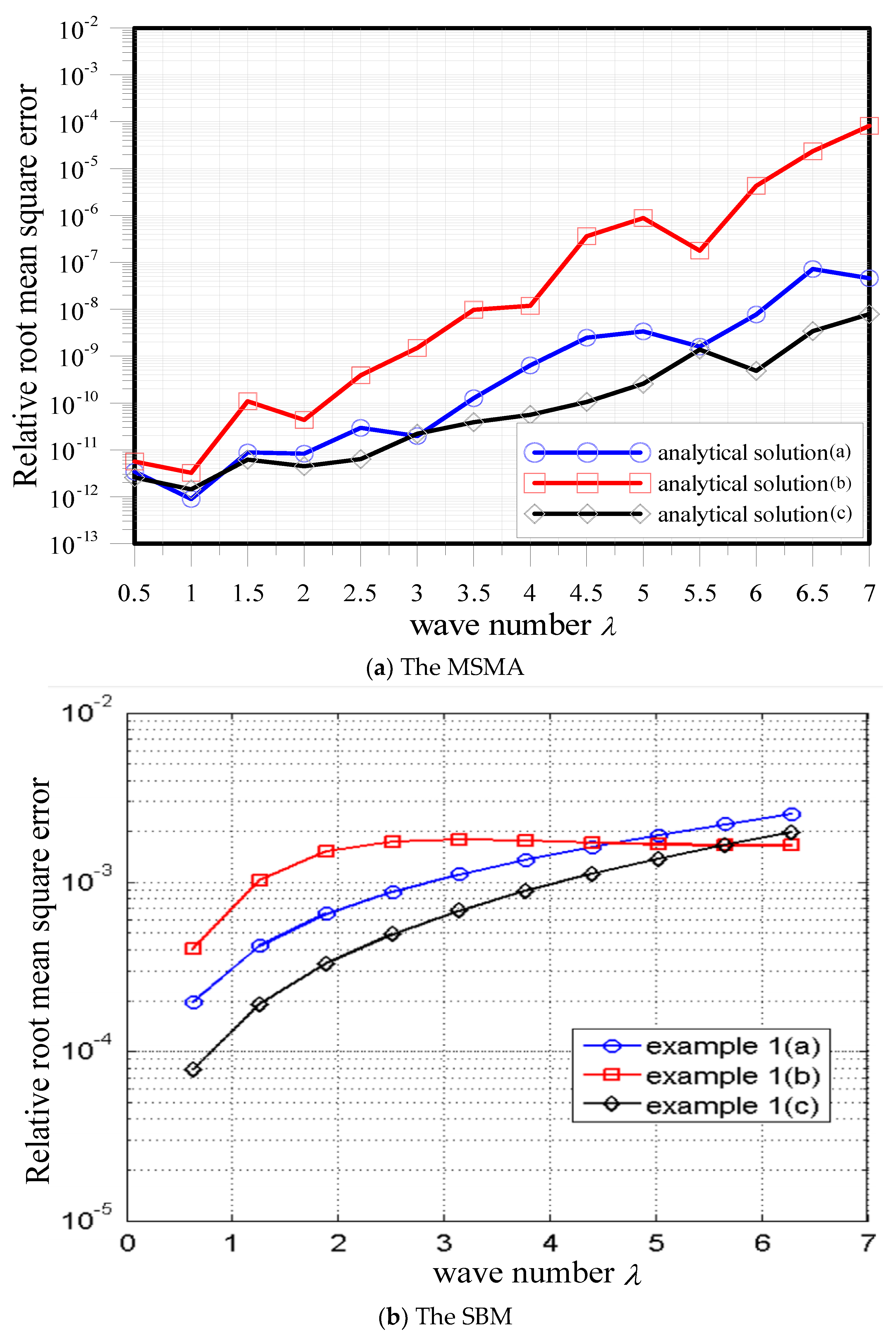
3.3. Investigation of the Wave Number

The third case is the modeling of the modified Helmholtz equation bounded by a peanut-shaped boundary, as depicted in Figure 10. To examine the effect of the wave number for the numerical results, different values of the wave number were considered in the example. The shape parameter of the irregular physical boundary is described by

$$\partial \mathsf{\Omega }=\left\{(x,y)|x=\rho (\theta )\cos (\theta ),y=\rho (\theta )\sin (\theta )\right\},$$

(30)

where $\rho =0.1\sqrt{\cos (2\theta )+\sqrt{1.1-\mathrm{si}{\mathrm{n}}^2(2\theta )}}$, and $0\le \theta \le 2\pi$.

To solve the modified Helmholtz equation, the exact solution can be found as

$$u={\mathrm{e}}^{(\sqrt{2}\lambda /2)(x-y)}.$$

(31)

The Dirichlet boundary values were imposed on the domain boundary using the exact solution. We investigated the accuracy of the proposed method by using different values of the wave number ranging from 1 to 50. Figure 10 shows the accuracy for the MAE versus the wave number using the proposed meshfree approach. As illustrated in Figure 10, the accuracy can be found in the order of ${10}^{-9}$ while $\lambda =50$. The numerical solutions revealed that the MSMA may yield highly accurate results even when the high wave number is considered.

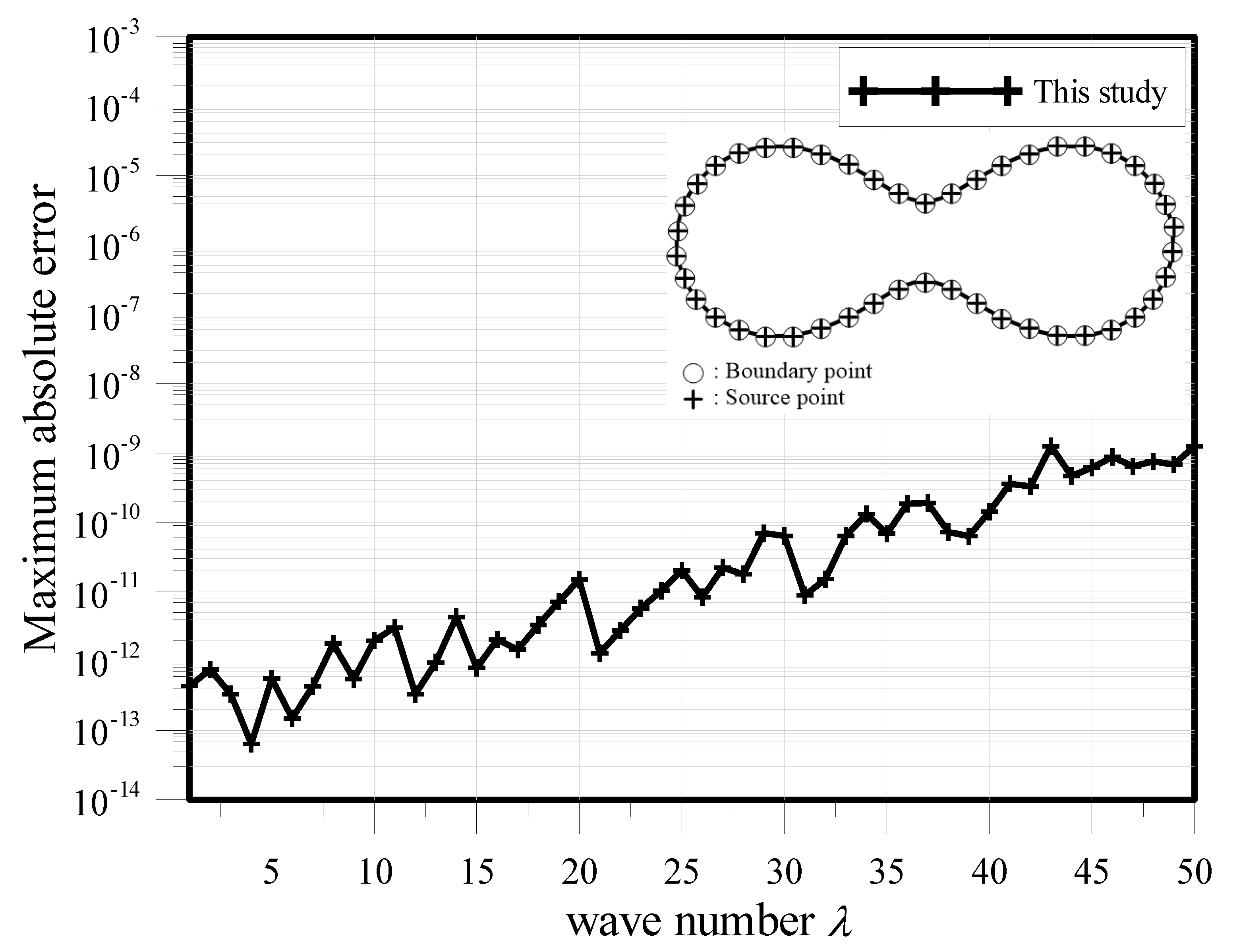
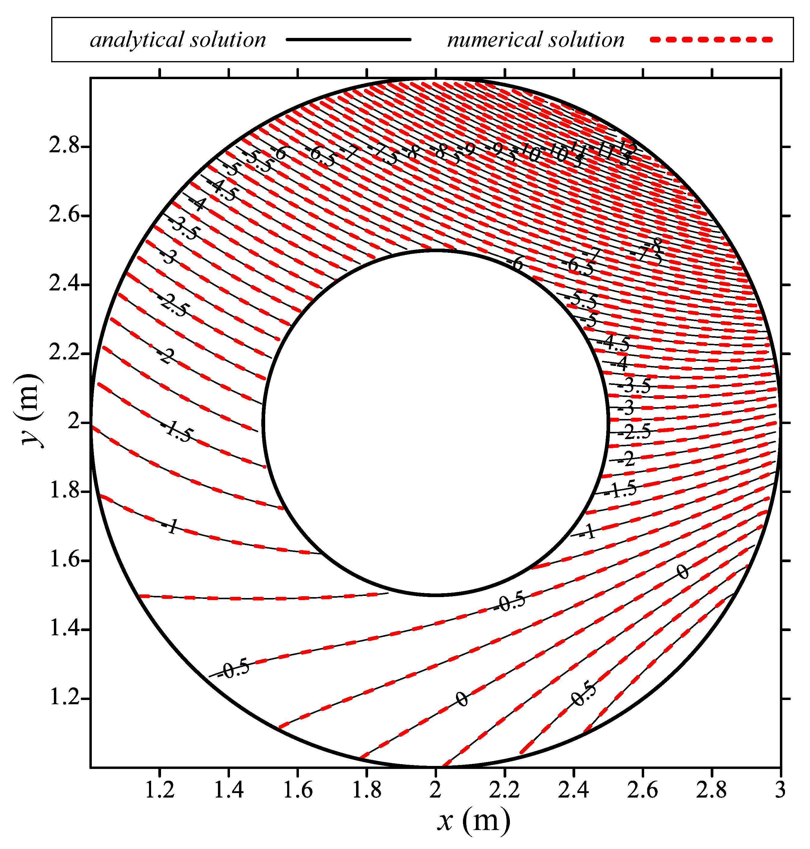
3.4. Solution of the Modified Helmholtz Equation Bounded by a Doubly Connected Region

The fourth case is the modeling of the modified Helmholtz equation bounded by a doubly connected region, as depicted in Figure 11. The shape parameter of the concentric circles is described by

$$\partial {\mathsf{\Omega }}_1=\left\{(x,y)|x={\rho }_1\cos {\theta }_1,y={\rho }_1\sin {\theta }_1\right\},{\rho }_1=1,$$

(32)

$$\partial {\mathsf{\Omega }}_2=\left\{(x,y)|x={\rho }_2\cos {\theta }_2,y={\rho }_2\sin {\theta }_2\right\},{\rho }_2=0.5.$$

(33)

The exact solution of this example can be found as follows:

$$u={\mathrm{I}}_3(k\rho )\cos (3\theta )+{\mathrm{K}}_3(k\rho )\cos (3\theta )$$

(34)

where ${\mathrm{I}}_3$ is the modified Bessel function of the third order for the first kind, and ${\mathrm{K}}_3$ is the modified Bessel function of the third order for the second kind. In this example, the terms of the particular solutions were set to be 15. The wave number was set as $\sqrt{2}$. For this example, the physical boundary, enclosed by a doubly connected region, was split into two simply connected subregions using the DDM [30,31], as depicted in Figure 11. Four hundred boundary and source points were interactively arranged on the physical boundary. Figure 12 shows that the sub-boundaries at the interface contained four sub-boundaries: ${\Gamma }_1$, ${\Gamma }_3$, ${\Gamma }_5$, and ${\Gamma }_7$. The overspecified boundary conditions enforced on the boundary and source points at the interface are described by

$${u|}_{{\Gamma }_1}={u|}_{{\Gamma }_5},{\frac{\partial u}{\partial n}|}_{{\Gamma }_1}={\frac{\partial u}{\partial n}|}_{{\Gamma }_5},{u|}_{{\Gamma }_3}={u|}_{{\Gamma }_7},{\frac{\partial u}{\partial n}|}_{{\Gamma }_3}={\frac{\partial u}{\partial n}|}_{{\Gamma }_7}.$$

(35)

To examine the accuracy, 2415 inner points were placed within the domain to obtain the numerical results. We also compared the numerical solutions with the above exact solution, as illustrated in Figure 13. It seems that the numerical solutions perfectly agree with the exact solution. Furthermore, the MAE of the MSMA can be obtained in the order of ${10}^{-6}$.

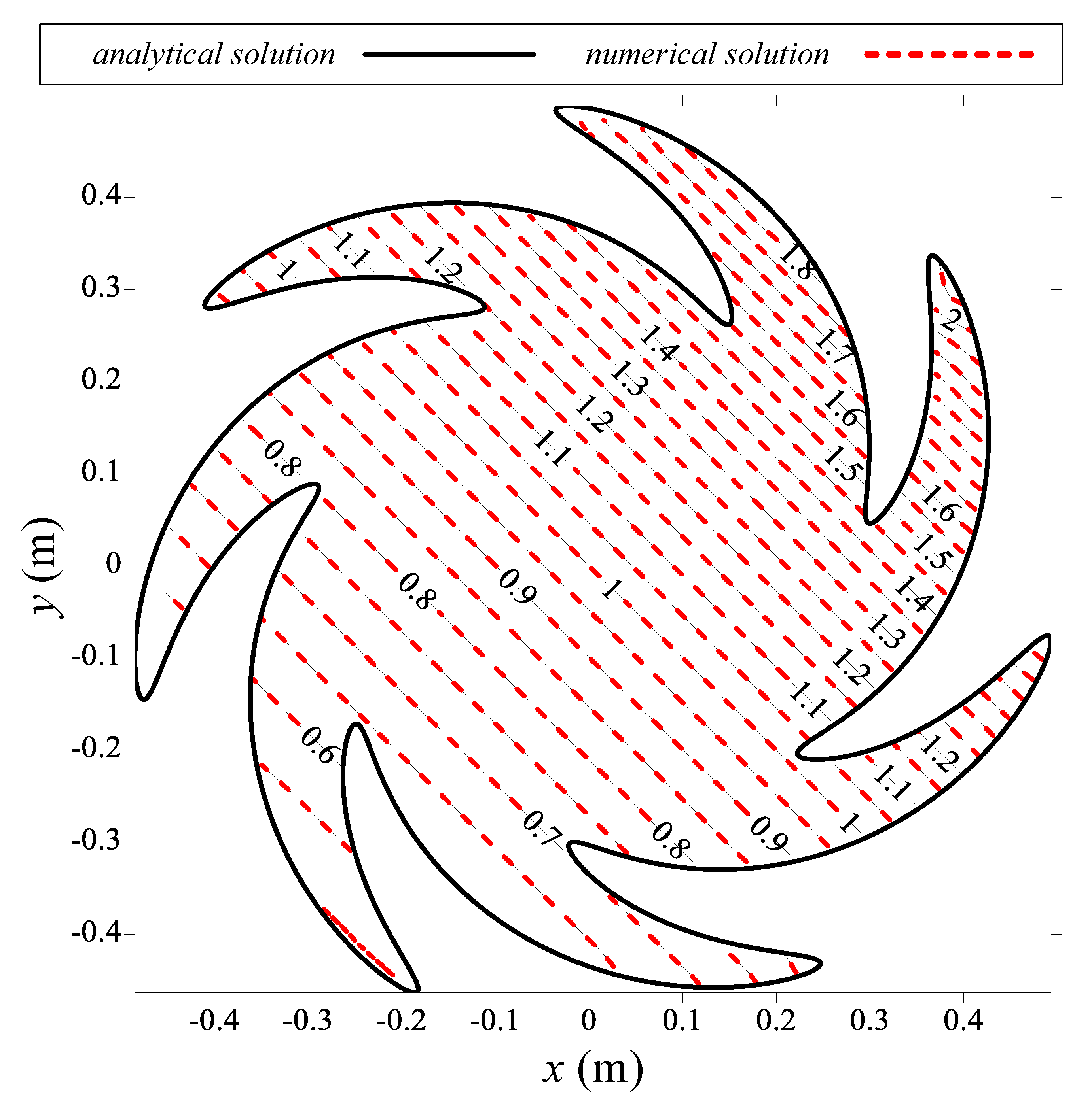
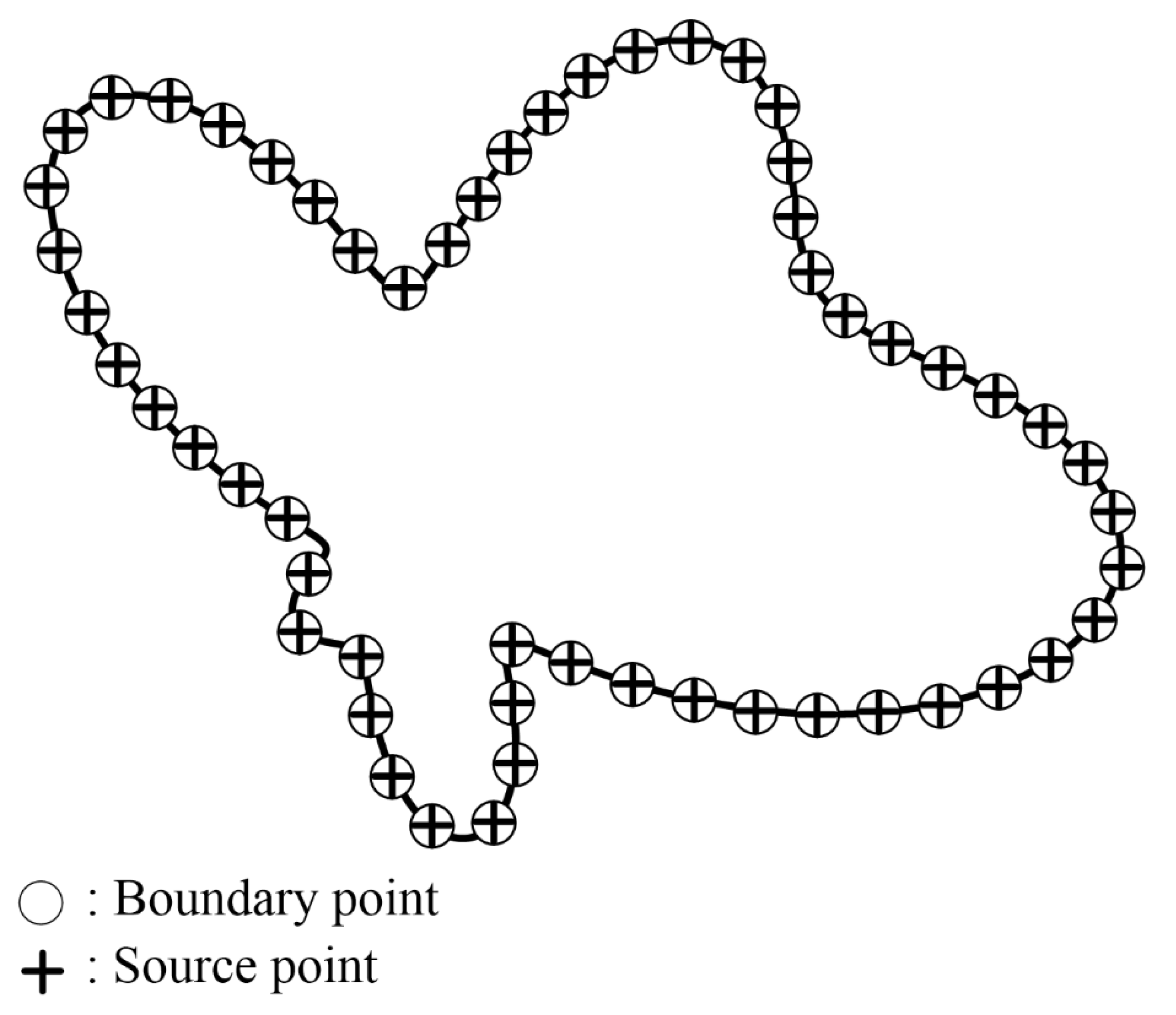
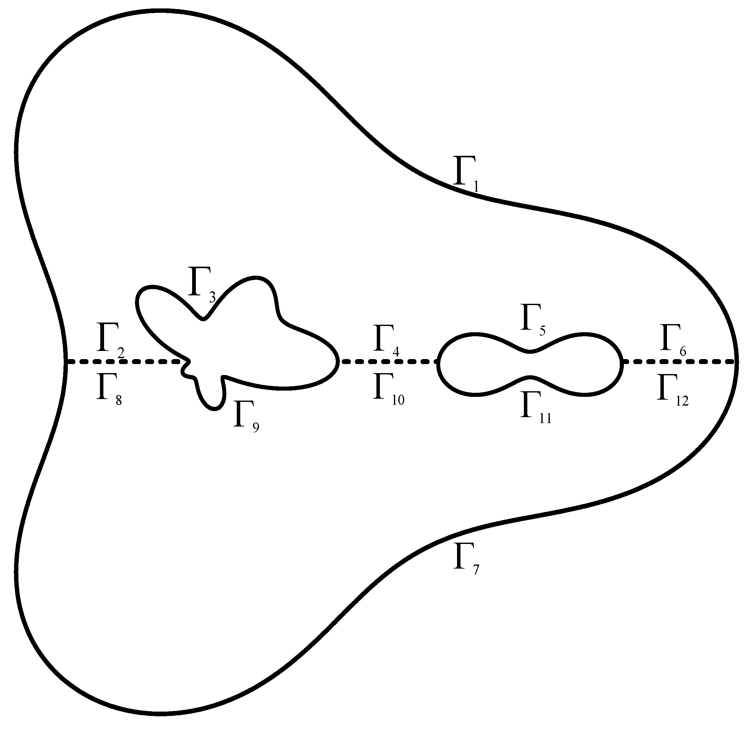
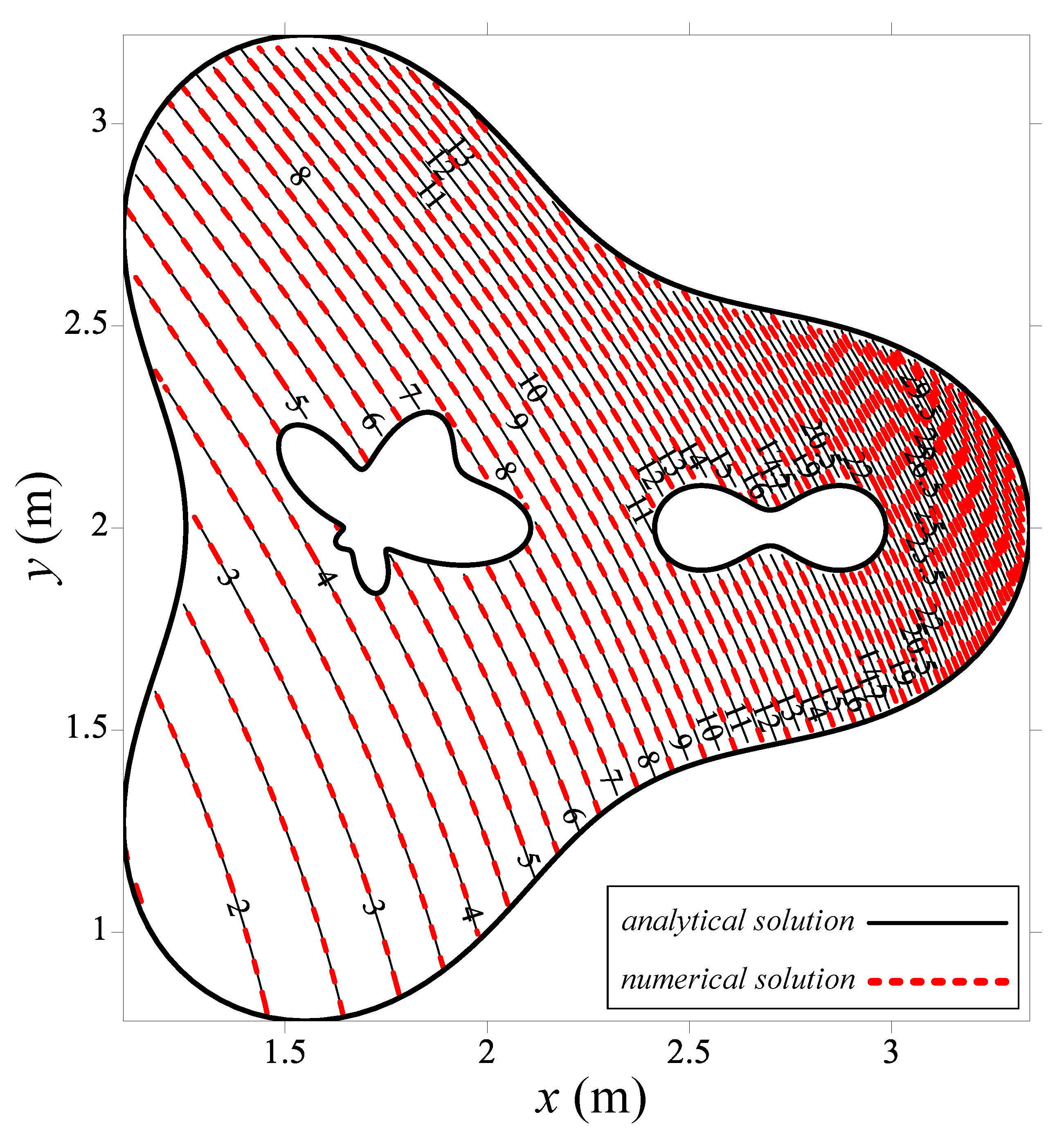
3.5. Solution of Modified Helmholtz Equation Bounded by a Multiply Connected Region

The fifth case is the modified Helmholtz equation bounded by a multiply connected region, as depicted in Figure 14. For the multiply connected domain including more than one cavity, we must place multiple source points within the physical boundary. Because the proposed MSMA does not consider the negative basis functions or the so-called singular basis functions, we cannot tackle the singular solution in the cavity by using only the nonsingular basis functions. Accordingly, to deal with problems bounded by multiply connected domains, the DDM was adopted, which split the domain into several simply connected subregions, such that we may guarantee subregions existing only in a nonsingular solution. The shape parameter of the physical boundary is given by

$$\begin{gathered} \partial {\mathsf{\Omega }}_1=\left\{(x,y)|x={\rho }_1\cos {\theta }_1,y={\rho }_1\sin {\theta }_1\right\},{\rho }_1={(\cos (3{\theta }_1)+\sqrt{2-{(\sin (3{\theta }_1))}^2})}^{1/3}, \\ 0\le {\theta }_1\le 2\pi , \end{gathered}$$

(36)

$$\partial {\mathsf{\Omega }}_2=\left\{(x,y)|x={\rho }_2\cos {\theta }_2,y={\rho }_2\sin {\theta }_2\right\},{\rho }_2={\mathrm{e}}^{{(\sin {\theta }_2\sin 2{\theta }_2)}^2}+{\mathrm{e}}^{{(\cos {\theta }_2\cos 2{\theta }_2)}^2},0\le {\theta }_2\le 2\pi ,$$

(37)

$$\begin{gathered} \partial {\mathsf{\Omega }}_3=\left\{(x,y)|x={\rho }_3\cos {\theta }_3,y={\rho }_3\sin {\theta }_3\right\},{\rho }_3=\sqrt{\cos (2{\theta }_3)+\sqrt{1.1-{(\sin (2{\theta }_3))}^2}}, \\ 0\le {\theta }_3\le 2\pi . \end{gathered}$$

(38)

The exact solution can be found as follows:

$$u={\mathrm{I}}_1(k\rho )\cos \theta +{\mathrm{K}}_1(k\rho )\cos \theta ,$$

(39)

where ${\mathrm{I}}_1$ is the modified Bessel function of the first order for the first kind, and ${\mathrm{K}}_1$ is the modified Bessel function of the first order for the second kind. In this example, the term of the particular solutions was 15. The wave number was set as $\sqrt{2}$. For this example, the physical boundary, enclosed by a doubly connected region, was split into two simply connected subregions using the DDM [30,31], as depicted in Figure 14. Four hundred boundary and source points were interactively arranged on the physical boundary. Figure 15 shows that the sub-boundaries at the interface contained six sub-boundaries: ${\Gamma }_2$, ${\Gamma }_4$, ${\Gamma }_6$, ${\Gamma }_8$, ${\Gamma }_{10}$, and ${\Gamma }_{12}$. The overspecified boundary conditions enforced on the boundary and source points at the interface are described by

$${u|}_{{\Gamma }_2}={u|}_{{\Gamma }_8},{\frac{\partial u}{\partial n}|}_{{\Gamma }_2}={\frac{\partial u}{\partial n}|}_{{\Gamma }_8},{u|}_{{\Gamma }_4}={u|}_{{\Gamma }_{10}},{\frac{\partial u}{\partial n}|}_{{\Gamma }_4}={\frac{\partial u}{\partial n}|}_{{\Gamma }_{10}},{u|}_{{\Gamma }_6}={u|}_{{\Gamma }_{12}},{\frac{\partial u}{\partial n}|}_{{\Gamma }_6}={\frac{\partial u}{\partial n}|}_{{\Gamma }_{12}}.$$

(40)

To examine the accuracy, 2737 inner points were placed within the domain to obtain the numerical results. We also compared the numerical solutions with the exact solution, as illustrated in Figure 16. The results demonstrate that the numerical solutions perfectly agree with the exact solution. Furthermore, the MAE of the MSMA can be obtained in the order of ${10}^{-6}$.

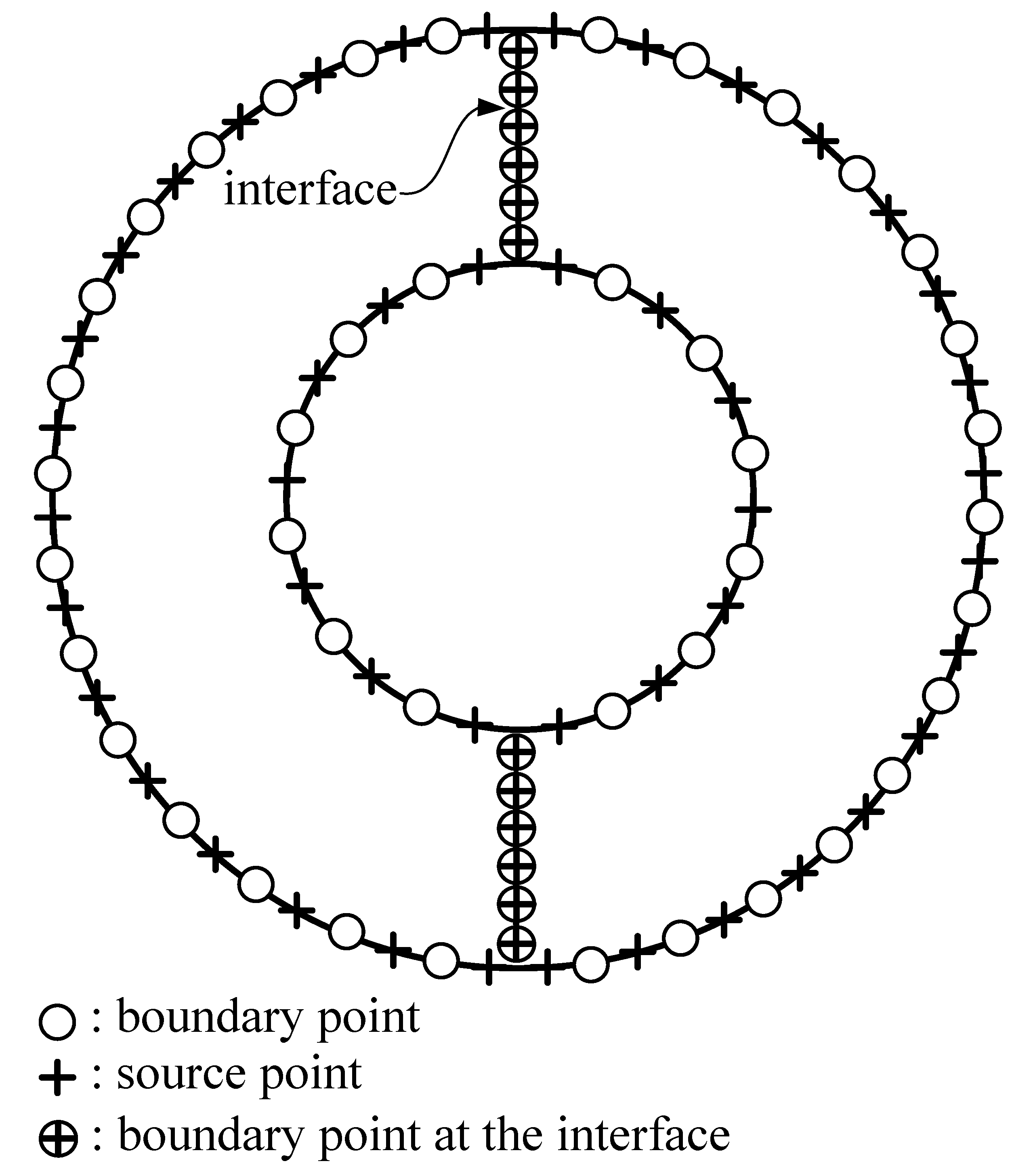
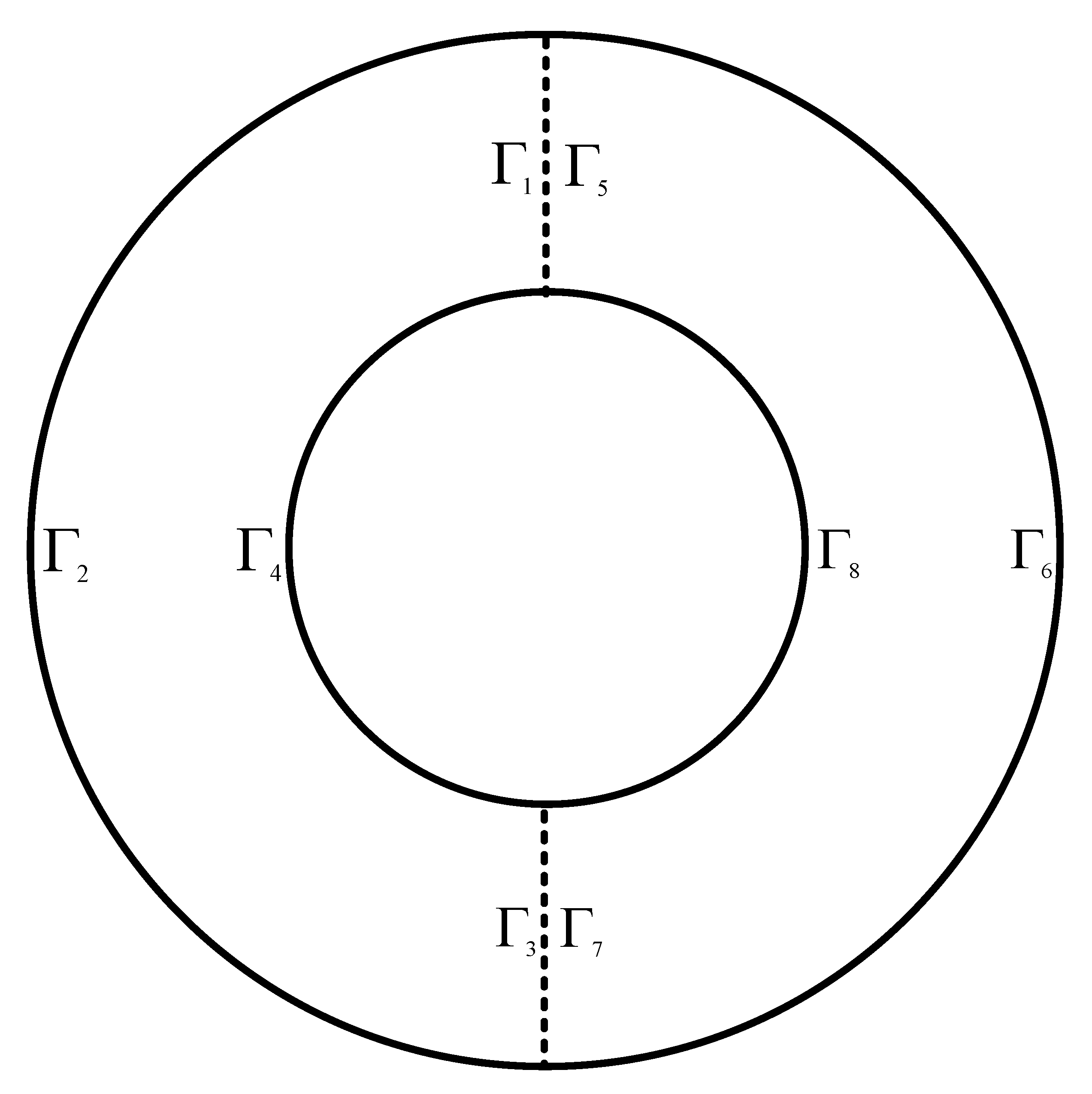
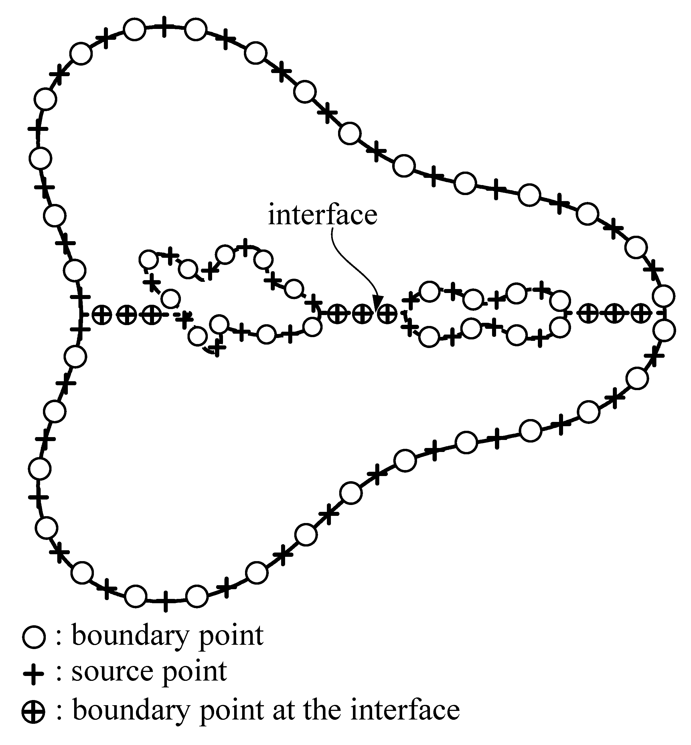
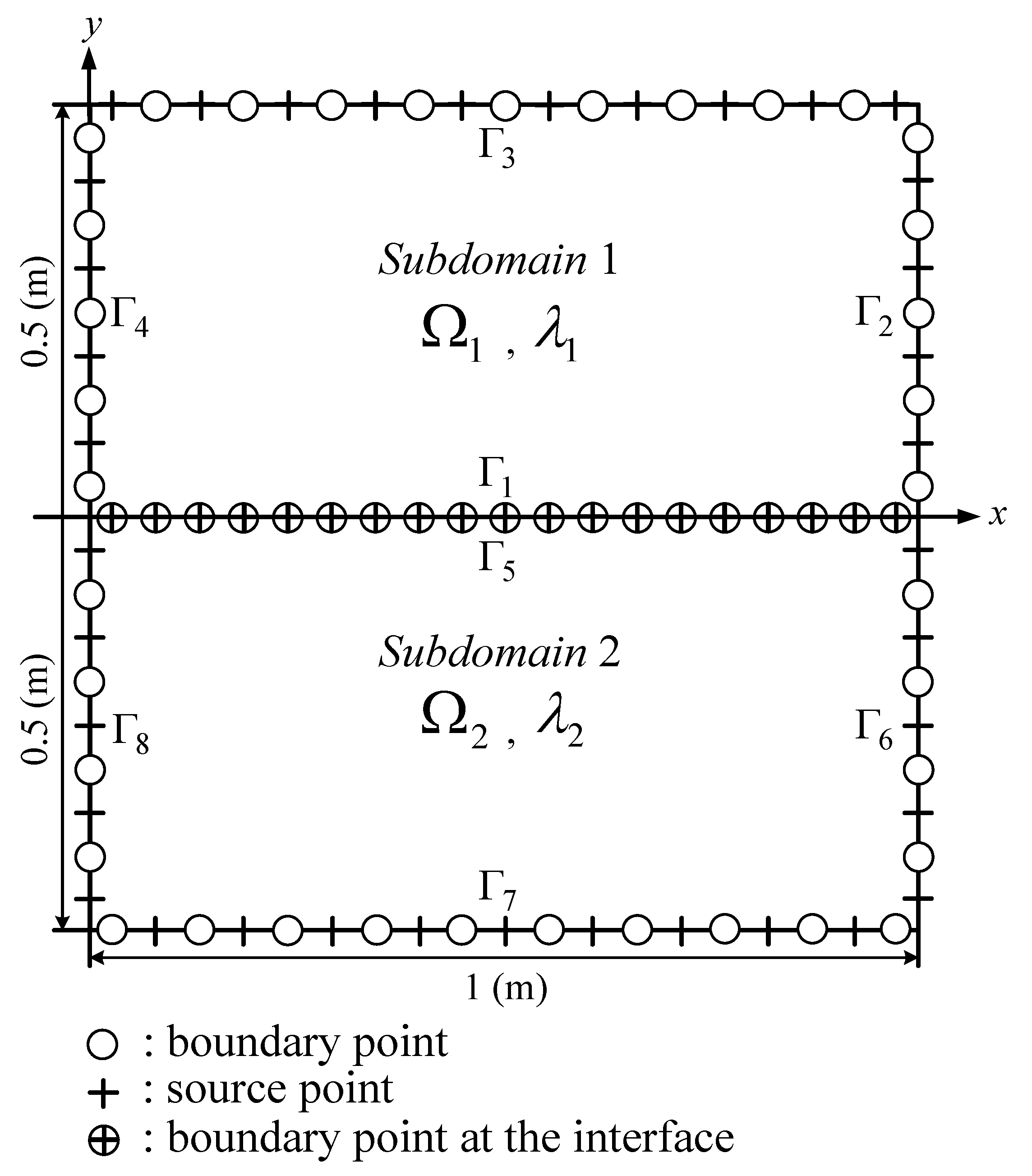
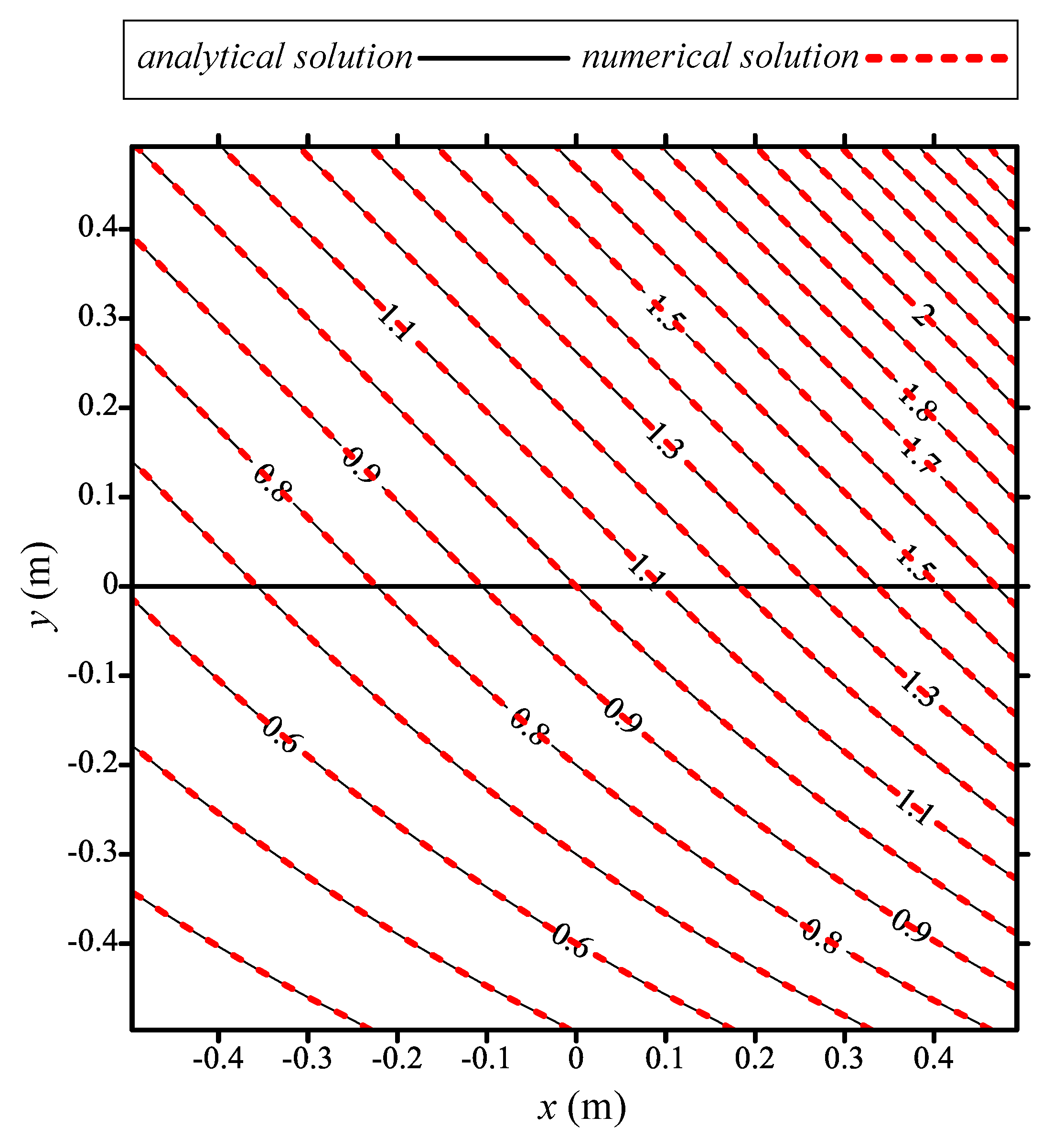
3.6. Solution of Modified Helmholtz Equation in Two Layered Materials

The last example is the modeling of the modified Helmholtz equation in two layered materials, as depicted in Figure 17. The wave number in two subdomains were set to be ${\lambda }_1$ and ${\lambda }_2$, in which ${\lambda }_1=\sqrt{2}$ and ${\lambda }_2=1$, respectively. The shape parameter of the boundary is described by

$$\partial {\mathsf{\Omega }}_1=\left\{(x_1,y_1)|0\le x_1\le 1,0\le y_1\le 0.5\right\},$$

(41)

$$\partial {\mathsf{\Omega }}_2=\left\{(x_2,y_2)|0\le x_2\le 1,0\le y_2\le -0.5\right\}.$$

(42)

The exact solutions are as follows:

$$u_1={\mathrm{e}}^{x+y},$$

(43)

$$u_2={\mathrm{e}}^x(1+y).$$

(44)

In this example, the terms of the particular solutions were 10. For modeling the modified Helmholtz equation in two layered materials, the physical boundary was split into two simply connected subregions using the DDM [30,31], as illustrated in Figure 17. For each subregion, 600 boundary and source points were interactively arranged on the physical boundary. Figure 17 also shows that the sub-boundaries at the interface contained two sub-boundaries: ${\Gamma }_1$ and ${\Gamma }_5$. The overspecified boundary conditions enforced on the boundary and source points at the interface are described by

$${u|}_{{\Gamma }_1}={u|}_{{\Gamma }_5},{\frac{\partial u}{\partial n}|}_{{\Gamma }_1}={\frac{\partial u}{\partial n}|}_{{\Gamma }_5}.$$

(45)

To evaluate the accuracy of the problem, 900 inner points were arranged within the domain to obtain the numerical results. We also compared the numerical solutions with the exact solution, as depicted in Figure 18. The results demonstrate that our results agree well with the above exact solution. Furthermore, we found that the MAE of the MSMA can be obtained in the order of ${10}^{-7}$, as depicted in Figure 19.

4. Discussion

In this paper, we proposed a multiple source meshfree approach for solving a two-dimensional modified Helmholtz equation in layered materials. The novel conception of the proposed MSMA started with the MFS and the CTM. The advantages of the proposed method are as follows.

The proposed method for solving the modified Helmholtz equation avoids a complicated procedure for finding the location of the sources. By adopting the nonsingular functions, the source points can be collocated on or within the domain boundary. Compared with other methods, highly accurate solutions can be obtained regardless of the location of source points. We also demonstrated that the proposed method incorporated with the DDM can be used to solve the modified Helmholtz equation in layered materials as well as the domain bounded by simply and multiply connected regions.

We investigated the accuracy of the proposed method by using different values of the wave number ranging from 1 to 50 for the modified Helmholtz equation. The accuracy of the MSMA was found in the order of ${10}^{-9}$, while the wave number was 50. The computed results revealed that the MSMA may yield highly accurate results even when a high wave number is considered. The proposed method is, however, limited for solving linear governing equations due to the approximation of the solution using the addition theorem.

5. Conclusions

In this study, we presented a meshfree approach for solving the modified Helmholtz equation bounded by simply, doubly, and multiply connected regions using the MSMA in two dimensions. The modified Helmholtz equation in two layered materials was also considered. The method was verified and numerical examples were also performed. We may point out the two major achievements of the paper:

• The key idea of the MSMA stems from the indirect boundary element method, which adopts multiple source points. Because of the adoption of nonsingular functions, the sources can be collocated on or within the domain boundary without using a complicated searching algorithm to find the appropriate location of the source points.
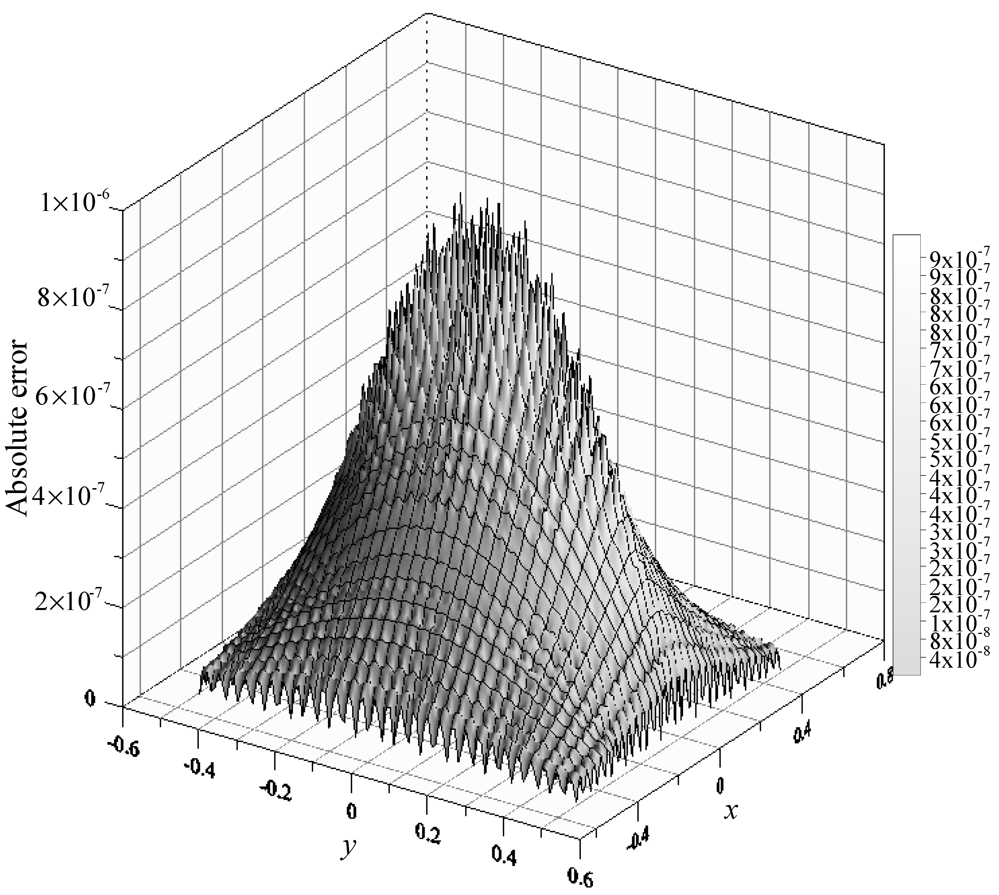
• To the best of our knowledge, the MSMA using nonsingular basis functions is newly developed. A pioneering work for solving the modified Helmholtz equation bounded by a multiply connected region was conducted using the MSMA in this study. Furthermore, the MAE of the proposed approach for the modified Helmholtz equation in two layered materials can reach up to the order of ${10}^{-7}$. From the computed results, we conclude that the MSMA is relatively simple because it avoids a complicated procedure for finding the appropriate location of the source points. Moreover, the MSMA has advantages of highly accurate and boundary collocation only for solving problems with complex geometry.

References

- Fan, C.M.; Liu, Y.C.; Chan, H.F.; Hsiao, S.S. Solutions of boundary detection problem for modified Helmholtz equation by Trefftz method. Inverse Probl. Sci. Eng. 2014, 22, 267–281. [Google Scholar] [CrossRef]
- Chen, K.H.; Chen, J.T.; Chou, C.R.; Yueh, C.Y. Dual boundary element analysis of oblique incident wave passing a thin submerged breakwater. Eng. Anal. Bound. Elem. 2002, 26, 917–928. [Google Scholar] [CrossRef]
- Nguyen, H.T.; Tran, Q.V.; Nguyen, V.T. Some remarks on a modified Helmholtz equation with inhomogeneous source. Appl. Math. Model. 2013, 37, 793–814. [Google Scholar] [CrossRef]
- Liu, C.S.; Qu, W.; Chen, W.; Lin, J. A novel Trefftz method of the inverse Cauchy problem for 3D modified Helmholtz equation. Inverse Probl. Sci. Eng. 2016, 25, 1278–1298. [Google Scholar] [CrossRef]
- Ben-Avraham, D.; Fokas, A.S. The Solution of the modified Helmholtz equation in a wedge and an application to diffusion-limited coalescence. Phys. Lett. A 1999, 263, 355–359. [Google Scholar] [CrossRef]
- Jleli, M.; Samet, B.; Vial, G. Topological sensitivity analysis for the modified Helmholtz equation under an impedance condition on the boundary of a hole. J. Math. Pures Appl. 2014, 103, 557–574. [Google Scholar] [CrossRef]
- Li, X. On solving boundary value problems of modified Helmholtz equations by plane wave functions. J. Comput. Appl. Math. 2006, 195, 66–82. [Google Scholar] [CrossRef]
- Yoneta, A.; Tsuchimoto, M.; Honma, T. An analysis of axisymmetric modified Helmholtz equation by using boundary element method. IEEE Trans. Magn. 1990, 26, 1015–1018. [Google Scholar] [CrossRef]
- Marina, L.; Lesnic, D.; Mantič, V. Treatment of singularities in Helmholtz-type equations using the boundary element method. J. Sound Vib. 2004, 278, 39–62. [Google Scholar] [CrossRef]
- Wang, R.; Chen, X. A fast solver for boundary integral equations of the modified Helmholtz equation. J. Sci. Comput. 2014, 65, 553–575. [Google Scholar] [CrossRef]
- Shen, D.J.; Lin, J.; Chen, W. Boundary knot method solution of Helmholtz problems with boundary singularities. J. Mar. Sci. Technol. 2014, 22, 440–449. [Google Scholar]
- Chen, W.; Hon, Y.C. Numerical investigation on convergence of boundary knot method in the analysis of homogeneous Helmholtz, modified Helmholtz, and convection-diffusion problems. Comput. Methods Appl. Mech. Eng. 2014, 192, 1859–1875. [Google Scholar] [CrossRef]
- Song, R.; Chen, W. A hybrid boundary node method. Int. J. Numer. Meth. Eng. 2002, 53, 751–763. [Google Scholar]
- Mukherjee, Y.X.; Mukherjee, S. A boundary node method for three-dimensional linear elasticity. Int. J. Numer. Meth. Eng. 1999, 46, 1163–1184. [Google Scholar]
- Chen, W.; Zhang, J.Y.; Fu, Z.J. Singular boundary method for modified Helmholtz equations. Eng. Anal. Bound. Elem. 2014, 44, 112–119. [Google Scholar] [CrossRef]
- Junpu, L.; Chen, W. A modified singular boundary method for three-dimensional high frequency acoustic wave problems. Appl. Math. Model. 2018, 54, 189–201. [Google Scholar]
- Ragusa, M.A. Cauchy-Dirichlet problem associated to divergence form parabolic equations. Commun. Contemp. Math. 2004, 6, 377–393. [Google Scholar] [CrossRef]
- Sun, L.; Chen, W.; Zhang, C. A new formulation of regularized meshless method applied to interior and exterior anisotropic potential problems. Appl. Math. Model. 2013, 37, 7452–7464. [Google Scholar] [CrossRef]
- Liu, L. Single layer regularized meshless method for three dimensional exterior acoustic problem. Eng. Anal. Bound. Elem. 2017, 77, 138–144. [Google Scholar] [CrossRef]
- Bin-Mohsin, B.; Lesnic, D. The method of fundamental solutions for Helmholtz-type equations in composite materials. Comput. Math. Appl. 2011, 62, 4377–4390. [Google Scholar] [CrossRef]
- Liu, C.S. Improving the ill-conditioning of the method of fundamental solutions for 2D Laplace equation. CMES-Comp. Model. Eng. 2008, 28, 77–93. [Google Scholar]
- Li, Z.C.; Huang, H.T.; Lee, M.G.; Chiang, J.Y. Error analysis of the method of fundamental solutions for linear elastostatics. J. Comput. Appl. Math. 2013, 251, 133–153. [Google Scholar] [CrossRef]
- Nishimura, R.; Nishimori, K.; Ishihara, N. Determining the arrangement of fictitious charges in charge simulation method using genetic algorithms. J. Electrost. 2000, 49, 95–105. [Google Scholar] [CrossRef]
- Karageorghis, A. A practical algorithm for determining the optimal pseudo-boundary in the method of fundamental solutions. Adv. Appl. Math. Mech. 2009, 1, 510–528. [Google Scholar] [CrossRef]
- Young, D.L.; Chen, K.H.; Chen, J.T.; Kao, J.H. A modified method of fundamental solutions with source on the boundary for solving Laplace equations with circular and arbitrary domains. CMES-Comp. Model. Eng. 2007, 19, 197–221. [Google Scholar]
- Liu, C.S. An equilibrated method of fundamental solutions to choose the best source points for the Laplace equation. Eng. Anal. Bound. Elem. 2012, 36, 1235–1245. [Google Scholar] [CrossRef]
- Shigeta, T.; Young, D.L.; Liu, C.S. Adaptive multilayer method of fundamental solutions using a weighted greedy QR decomposition for the Laplace equation. J. Comput. Phys. 2012, 231, 7118–7132. [Google Scholar] [CrossRef]
- Ku, C.Y.; Xiao, J.E.; Liu, C.Y.; Fan, C.M. On modeling subsurface flow using a novel hybrid Trefftz-MFS method. Eng. Anal. Bound. Elem. 2019, 100, 225–236. [Google Scholar] [CrossRef]
- Xiao, J.E.; Ku, C.Y.; Huang, W.P.; Su, Y.; Tsai, Y.H. A novel hybrid boundary-type meshless method for solving heat conduction problems in layered materials. Appl. Sci. 2018, 8, 1887. [Google Scholar] [CrossRef]
- Boubendir, Y.; Midura, D. Non-overlapping domain decomposition algorithm based on modified transmission conditions for the Helmholtz equation. Comput. Math. Appl. 2018, 75, 1900–1911. [Google Scholar] [CrossRef]
- Meric, R.A. Domain decomposition methods for Laplace’s equation by the BEM. Commun. Numer. Meth. Eng. 2000, 16, 545–557. [Google Scholar] [CrossRef]
© 2019 by the authors. Licensee MDPI, Basel, Switzerland. This article is an open access article distributed under the terms and conditions of the Creative Commons Attribution (CC BY) license (http://creativecommons.org/licenses/by/4.0/).
Share and Cite
Ku, C.-Y.; Xiao, J.-E.; Yeih, W.; Liu, C.-Y. On Solving Modified Helmholtz Equation in Layered Materials Using the Multiple Source Meshfree Approach. Mathematics 2019, 7, 1114. https://doi.org/10.3390/math7111114
Ku C-Y, Xiao J-E, Yeih W, Liu C-Y. On Solving Modified Helmholtz Equation in Layered Materials Using the Multiple Source Meshfree Approach. Mathematics. 2019; 7(11):1114. https://doi.org/10.3390/math7111114
Chicago/Turabian StyleKu, Cheng-Yu, Jing-En Xiao, Weichung Yeih, and Chih-Yu Liu. 2019. "On Solving Modified Helmholtz Equation in Layered Materials Using the Multiple Source Meshfree Approach" Mathematics 7, no. 11: 1114. https://doi.org/10.3390/math7111114
APA StyleKu, C.-Y., Xiao, J.-E., Yeih, W., & Liu, C.-Y. (2019). On Solving Modified Helmholtz Equation in Layered Materials Using the Multiple Source Meshfree Approach. Mathematics, 7(11), 1114. https://doi.org/10.3390/math7111114